P. Ashok*![]() | B. Latha
| B. Latha![]()
© 2024 The authors. This article is published by IIETA and is licensed under the CC BY 4.0 license (http://creativecommons.org/licenses/by/4.0/).
OPEN ACCESS
Finding underwater sound sources is quite difficult because of how complex and interconnected the undersea world is. When trying to use ship-radiated noise for Underwater Acoustic Target Recognition (UATR), the complicated presence of aquatic creatures makes the process even more tough. An innovative DNN called the Audio Perspective Region-based Convolutional Neural Network (APRCNN) is presented in this study. In order to train APRCNN, we used Depth Wise Separable (DWS) Convolutional Deep Neural Network architecture using initial underwater acoustic wave data. After that, APRCNN is used to categories and forecast underwater sound waves. Novel aspects of the suggested APRCNN model include optimization, adaptive learning, processing in parallel with residual connections, and underwater environment adaptation. With the help of integration layers that were influenced by the perceptual processing of the SPDNN system. Machine translation approaches also improve the model's performance through the use of time-dilated convolution. In this research, we offer a technique for underwater target detection with a full-featured DNN architecture. To achieve optimal classification accuracy with minimal compute load in different underwater degradation conditions, the suggested architecture maximizes the reallocation of prior feature maps. In addition, the suggested method eliminates the requirement for time-frequency spectrum analyzer pictures by allowing the network to be fed real data from audio signals instead. With a remarkable 98.4 percent accuracy level at 0-dB Signal to Noise Ratio (SNR), our classification methodology outperforms both state-of-the-art DNN systems and classic ML approaches, as demonstrated by thorough examination of a real-world dataset of passive sonar waves. When compared to other DNN systems for processing underwater acoustic signals, PRCNN stands out due to its adaptive learning mechanisms, focus on perspective regions, integration of domain knowledge, learning of hierarchical representations, resilience to environmental variability, and region-specific feature extraction. Thanks to these upgrades, APRCNN is now better able to identify, classify, and localize sounds in underwater acoustic settings, as well as to handle the unique problems of underwater signal processing.
features extractor, image processing, underwater acoustic, Region-based Convolutional Neural Network, ship-radiated noise, target recognition
The complicated and tough environment makes it difficult to discover underwater communication sources. Shallower classifiers, which may include variables that were hand-designed, are used in traditional machine-learning approaches to underwater audio target detection [1]. Scientists retrieve the manually specified properties of ship-transmitted noise using time frequency, spectrum, wavelet transform, and a few other features [2, 3]. The generalizability of these manually-created traits is poor since they rely on past and specialized information. On the other hand, traditional underwater acoustic target monitoring methods exhibit subpar concordance and generalization when confronted with massive amounts of complicated data [4]. The current method of underwater sound detection is thus mostly carried out by trained sonars. Underwater target recognition using Deep Learning (DL) techniques has been a hot topic as of late. From the ship's radiant sound spectrogram, researchers used a stacking auto-encoder and flexible-max classification to extract deep properties [5]. Deep learning and deep neural network models may be used to extract deep information from radiation noise spectra of ships. The researchers combined Deep Belief Networks (DBN) with competitive learning approaches to create a Deep Beliefs network that is competitive.
Underwater photography is crucial to the success of oceanographic mechanical vision applications like marine animal detection and geotechnical environment evaluation (which includes underwater archaeology). Getting a good grasp of depth is challenging in relation to the physiological features of aquatic environments. There are a number of technological and scientific challenges to oil and gas extraction from undersea sources. Constant monitoring is necessary for all pipelines carrying natural gas and oil. For the purpose of testing underwater pipes, human intervention was necessary for the operation of remotely operated vehicles (ROVs). This is a highly risky procedure, I'm afraid. The solution, then, is to harness the power of an aqueous electrolyte with an efficient way for perceptual objective tracking and identification approaches to aid human endeavors through intelligent perception navigation and guiding. The ROVs were self-sufficient underwater vehicles that were affixed to the ship's exterior via electrical cables in order to enable them to operate kilometers below the ocean's surface. Underwater things might be examined and fixed using these. Instructions and data can be sent and received with the help of these leads. Using a controller, the ROV may be operated by trained operators at a control station who observe all it observes. Spending a lot of effort and money on this kind of strategy necessitates hiring people with certain training. Recording equipment mounted to the ROV took pictures of the underwater environment, which were then reviewed by a second operator who was able to spot almost any anomaly.
It is possible that the recognition performance will be better using the DL approaches discussed above compared to more traditional methods. On top of that, none of those methods really shed light on the time-frequency aspects of vessel noises. Though the method's recognition rate was greater than expected, it was not without its shortcomings. For example, it performed poorly in input audio circumstances and had trouble with the Discrete Fourier Transform (DFT) utilized for domain conversion. Deep learning (DL) has recently gained traction in the classification of underwater acoustic waves and has accomplished remarkable feats in other research fields, including machine learning and bioinformatics. To improve identification accuracy by removing superfluous features, one can train the fusion characteristic of the gammatone frequencies cepstrum coefficients and enhanced empirical mode reduction in a DNN using a Gaussian mixture modelling level. Also examined for vessel acknowledgment was a multimodal DL approach based on ship-radiated audio. This method has the possibility to improve sonar systems by combining feature representations obtained from visual and aural approaches at an intermediate stage, which might increase their accuracy and reliability.
The training process for feature extraction of underwater acoustic signal targets using machine learning techniques typically involves several steps, along with specific machine learning algorithms and methodologies employed. Here's an overview:
Data Collection and Preprocessing: Acquire a dataset of underwater acoustic signals containing recordings of various target classes (e.g., marine vessels, aquatic animals) and environmental conditions. Preprocess the raw data to remove noise, filter out irrelevant frequencies, and normalize the signals to ensure consistency across samples.
Feature Extraction: Extract relevant features from the pre-processed acoustic signals that are indicative of different target classes or phenomena. Commonly used feature extraction techniques include:
Time-domain Features: Statistical measures such as mean, variance, skewness, and kurtosis of signal amplitudes over time intervals.
Frequency-domain Features: Spectral characteristics obtained through Fourier transform-based methods, including power spectral density, spectral centroid, and spectral bandwidth.
Time-frequency Domain Features: Extracted using techniques such as wavelet transforms, spectrogram analysis or short-time Fourier transforms to capture temporal variations in frequency content.
Model Selection: Choose appropriate machine learning models capable of learning from the extracted features to perform target detection and classification. Commonly employed machine learning techniques for feature extraction in underwater acoustic signal processing include:
Support Vector Machines (SVM): Supervised learning models used for binary or multiclass classification by finding hyperplanes that best separate classes in the feature space.
Random Forests: Ensemble learning methods that construct multiple decision trees during training and output the class that is the mode of the classes output by individual trees.
Convolutional Neural Networks (CNNs): Deep learning architectures designed to automatically learn hierarchical feature representations from input data, commonly used for image and signal processing tasks.
Recurrent Neural Networks (RNNs): Neural network architectures suitable for sequential data processing, often used for time-series analysis and sequence prediction tasks.
Model Training: If you want to train and test different machine learning models, you need to partition the dataset into two parts: training and validation.
Train the models using the training data while monitoring to avoid overfitting by evaluating performance on the validation set. While training, minimize the loss function by using suitable optimization techniques (such as Adam or stochastic gradient descent) to update the model's parameters.
Hyperparameter Tuning and Optimization: To get the best results, tweak the models' hyperparameters (such learning rate and regularization parameters). To find the best settings for your hyperparameters, use methods like grid search, random search, or Bayesian optimization.
Model Evaluation: Apply measures like F1-score, accuracy, precision, recall, and receiver operating characteristic (ROC) curve analysis to a different test set to assess how well the trained models performed. Make that the trained models can successfully categories underwater acoustic waves in real-world circumstances and generalize well to unseen data.”
Researchers and practitioners may train models for feature extraction of underwater acoustic signal targets by following these steps and utilizing specialized machine learning techniques like SVMs, Random Forests, CNNs, and RNNs. Marine surveillance, underwater communication, and environmental monitoring are just a few of the many important applications that rely on these models to accurately identify and categories underwater targets.
Key contributions of this research would include:
1. Using a model built from feature extraction convolutional networks, this paper proposes a completely convolutional filter comment thread to imitate the architecture of gathering depth wise frequency content in an auditory ecosystem.
2. Based on the way the brain detects the carrier frequency, we deconstructed and modelled the complex frequency component of ship-radiated sound using a set of multi-scale filter subnetworks of the depth's separable convolutions.
3. The language modelling technique drove the usage of time-dilated convolution to extract functional and cross data for UATR.
4. The experimental findings demonstrate that the APRCNN framework that was suggested worked well for UATR. Deconstructing, modelling, and classifying ship-radiated additive noise has never been easier than with this method, which outperformed competing methods.
1.1 Problem statement
Underwater environments present unique challenges for the detection and classification of acoustic signals emitted by various sources such as marine vessels, aquatic animals, and environmental phenomena. One of the critical tasks in underwater acoustic signal processing is feature extraction, which involves capturing relevant information from the raw acoustic signals to facilitate accurate target detection and classification.
However, feature extraction from underwater acoustic signals is challenging due to factors such as signal attenuation, multipath propagation, ambient noise, and the presence of marine life. Traditional feature extraction methods may not adequately capture the distinctive characteristics of underwater acoustic signals, leading to reduced detection and classification performance.
This research aims to address the following key aspects related to the feature extraction of underwater acoustic signal targets:
Identification of Discriminative Features: Investigate and identify the most discriminative features within underwater acoustic signals that are indicative of specific targets or phenomena. This involves analyzing the spectral, temporal, and spatial characteristics of the signals to identify features that can effectively differentiate between different underwater targets.
Development of Robust Feature Extraction Techniques: Develop novel feature extraction techniques that are robust to environmental variations and noise commonly encountered in underwater environments. This includes exploring advanced signal processing algorithms, such as wavelet transforms, time-frequency analysis, and adaptive filtering, to extract robust features from noisy underwater acoustic signals.
Integration of Machine Learning Techniques: Explore the integration of machine learning techniques, such as deep learning architectures, into the feature extraction process to automatically learn discriminative features from raw acoustic signals. This involves designing and training deep neural networks specifically tailored for underwater acoustic signal processing, capable of extracting hierarchical representations of the input signals.
Evaluation of Feature Extraction Performance: Evaluate the performance of the proposed feature extraction techniques in terms of their ability to accurately capture relevant information from underwater acoustic signals. This involves conducting comprehensive performance evaluation experiments using real-world underwater acoustic datasets, considering metrics such as detection accuracy, classification performance, and robustness to noise and environmental variability.
By addressing these aspects, this research aims to advance the state-of-the-art feature extraction of underwater acoustic signal targets, ultimately contributing to improved detection and classification capabilities in various underwater applications such as marine surveillance, underwater communication, and environmental monitoring.
Using AUVs (Autonomous Underwater Vehicles) with little human intervention might save time and money. The AUV needs efficient and reliable systems for localization [6]. This calls for smart object-tracking methods due to the scenario's repeating nature and the requirement for long-term, continuous analysis. A recording device and radar can be used to identify and check pipelines that protrude out of the earth. If a satellite service exists, then magnetization is a determining factor. Nevertheless, it is not able to supply any data, especially in cases when the pipe is subterranean or extended beyond the surface [7]. It is possible to capture images of underwater objects using a sub-benthic scanner. The presence of an underwater pipeline, as well as the kind and depth of silt, may be confirmed using this method [8]. Locating, finding, and monitoring submerged or protruding underwater pipelines is made possible by a combination of magnetization, raised sub-bottom profiling, dual-frequency side-scan radar, and a high-resolution sub-bottom analyzer.
A subsurface sensor system may prove to be highly beneficial for AUVs [9]. Terrestrial, marine, and extraterrestrial travel can all benefit from visual navigation technologies. Video captures more information at a lower cost than microphones. Notable among image categorization paradigms is the Region-based Convolutional Neural Network (RCNN) [10]. After scanning the image, the algorithms come up with around 2,000 possible zones that are unrelated to the original photos' categories. Using a computation template, create characteristic maps from each target region that are the same size. After that, get a Support Vector Machine (SVM) [11] and find all the potential regions' category entries. For every screen that qualifies, this R-CNN approach uses algebraic image distortion to determine the inputs of a completely Convolutional with a constant size, regardless of its appearance. The object detection success rate of Quick R-CNN and Rapid R-CNN, both of which are R-CNN based, is significantly higher [12-15]. The R-CNN model, upon which this Fast R-CNN is built, incorporates the.net programmed features to enhance modelling sensing capabilities and speed up supervised learning.
As a whole, there are two components to fast R-CNN detection [16]. The first stage is to create a category classifier using the complete picture as inputs and a fully Convolutional Regional Proposal Network (RPN) [17]. The second phase involves classifying networks, which basically divides entrance proposals into several classifiers. These two difficulties have a foundation in the same completely linked layers.
In order to evaluate harmonic frequencies, the main sensory centre uses nerve fibers with an input vector that has several scale components to break complicated auditory signals into many frequencies [18]. In addition, different frequency components of acoustic waves can elicit diverse responses from the auditory system. An individual's optimal learning speed and the amount of sound parameters are both affected by the regions of the brain responsible for frequency identification, which include the auditory cortex, auditory midbrain, and the hearing centre [19]. Based on these findings, it seems that the auditory pathway's time-domain acoustic data might be separated into spectrum analysis [20]. One possible interpretation of frequency content fragmentation in frequency-domain acoustic signals is as a filtering product [21]. In order to evaluate and categories acoustic signals, the nervous system receives information from all areas of the auditory pathway, and each area of the pathway interprets a unique component of frequency [22-24]. Due to the fact that a spatial frequency transmitter's item is analogous to a time domain convent signal, the speed element might be efficiently achieved by means of time-domain complexity parallel processing.
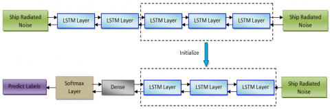
Working in tandem, the Denoising Auto Encoder (DAE) nodes and the DL Memory Network (DLMN) system are the suggested operational DL. Figure 1 shows the two-step process that is suggested. Researchers begin by constructing an LSTM-based DAE network, which is used for both encoding and decoding. The goal of the LSTM-based DAE network was to implement a DLMN model into the DAE system using an uncontrolled learning technique. You can decrease the input size by adding LSTM layers one at a time. The encoder additionally incorporates one or more LSTM layers for the purpose of reconstructing the model parameters. Stage two involved constructing a cooperative DLMN network from the LSTM-based DAE network's pre-formed encoding and the soft-max classification. The goal of the DLMN Cooperation Network's reinforcement techniques is to classify and describe ship-radiated noise.
Figure 1. The DL architecture
The long short-term memory (LSTM) network's flexible replication circuits, which may have two or more synaptic connections, are based on the memory block and choose when to retrieve and store data from a master memory [25]. In order to control the cell's stimulation, the three gateways used fundamental mathematics to combine action potentials from within and outside the block. The memory controller twice the cell's previous state, while the input and output doors double the cell's inputs and outputs. LSTM cells are able to access and retain data for long periods of time because of the exponential gate. The LSTM network takes scenes as input and output, which are actually collections of vector models across time. One output of the LSTM network is linked to the other output and the current input. The structural arrangement of the LSTM is shown in Figure 2.
Figure 2. The structure of LSTM
"We can get the flowing iterative equations by setting the input, hidden layer, and output of the LSTM to $i=i-1 ., i-2 ., \ldots, i-n ., h=, h-1 ., h-2 ., \ldots, h-$ $n$., and $b=a-1 ., a-2 ., \ldots, b-n . "$
${{h}_{t}}=H\left( {{W}_{h}}.\left[ {{h}_{t-1}},{{i}_{t}} \right]+{{b}_{h}} \right)$ (1)
$j_t=W_j \cdot h_t+b_j$ (2)
If $\mathrm{t}=1,2, \ldots, n$, then $W$ is the weight matrix, $\mathrm{b}$ is the bias. A composite function of hidden layers, $H$, can be iterated using the following formulae.
${{f}_{t}}=\sigma \left( {{W}_{f}}.\left[ {{h}_{t-1}},{{i}_{t}} \right]+{{b}_{f}} \right)$ (3)
${{x}_{t}}=\sigma \left( {{W}_{t}}.\left[ {{h}_{t-1}},{{i}_{t}} \right]+{{b}_{x}} \right)$ (4)
${{\hat{g}}_{t}}=\tan h\left( {{W}_{g}}.\left[ {{h}_{t-1}},{{i}_{t}} \right]+{{b}_{g}} \right)$ (5)
${{C}_{t}}={{f}_{t}}.{{C}_{t-1}}+{{x}_{t}}.{{\hat{g}}_{t}}$ (6)
${{o}_{t}}=\sigma \left( {{W}_{o}}.\left[ {{h}_{t-1}},{{i}_{t}} \right]+{{b}_{o}} \right)$ (7)
${{h}_{t}}={{o}_{t}}.\tan h\left( {{C}_{t}} \right)$ (8)
where, $f_{\mathrm{t}}$. is the forgotten gate, $x_t$ and $g_{\mathrm{t}}$ are the input gate, $o_{\mathrm{t}}$. is the output gate, and $c_t$ is the cell state $\sigma$(.) is the sigmoid activation function and the expression of $\sigma$(.), tanh-(.) are as follows:
$\sigma \left( i \right)=\frac{1}{1+{{e}^{-i}}}$ (9)
Step two, looking at it from a positive angle, is to construct a cooperative DLMN network. A learning algorithm and a pre-formed receptor level make up this architecture. The learning step involves training and optimizing the cooperative DLMN networks' variables, which are first set by the LSTM-based DAE networks. Through the use of variation and intrinsic feature learning, the cooperative DLMN system is able to reflect latent categories [26]. The categorization systems are composed of a number of variables whose frequency, throughout time, change. The characteristics acquired by LSTM-based DAE networks, which store valuable classification data, can enhance the precision of underwater target acoustic monitoring.
3.1 Dataset description
The dataset utilized for evaluating the proposed model consists of underwater acoustic signals collected from diverse marine environments and conditions. The dataset was curated to encompass a wide range of underwater acoustic phenomena and target classes, including marine vessels, aquatic animals, and environmental sounds.
Size and Diversity: The dataset comprises a substantial number of acoustic signal recordings, totaling 21.7 hours of underwater audio data. Signals were captured using hydrophones deployed in various underwater locations, including coastal regions, open ocean environments, and marine reserves. To ensure diversity, recordings were obtained under different weather conditions, water depths, and times of day to capture variations in environmental factors and acoustic propagation characteristics.
Representation of Target Classes: The dataset includes recordings of diverse underwater targets, including but not limited to:
Marine vessels: Ships, boats, submarines.
Aquatic animals: Marine mammals, fish, crustaceans.
Environmental sounds: Waves, wind, rain, anthropogenic noise. Each target class is represented by a sufficient number of instances to enable robust evaluation of the model's performance across different classes.
Ground Truth Labeling: Ground truth labels were manually annotated by domain experts to ensure accuracy and reliability. Annotations include information about the presence, type, and location of underwater targets within the audio recordings.
Relevance and Adequacy for Evaluation: The dataset was carefully curated to be representative of real-world underwater acoustic scenarios, ensuring that the evaluation reflects the challenges and complexities encountered in practical applications. By encompassing a diverse range of target classes and environmental conditions, the dataset provides a comprehensive testbed for evaluating the proposed model's performance across different underwater acoustic contexts. The size and diversity of the dataset enable rigorous evaluation of the model's generalization capabilities and robustness to variations in acoustic conditions and target classes.
Discussion: The dataset used for evaluation is well-suited for assessing the proposed model's performance in real-world underwater acoustic signal processing tasks. However, it is important to acknowledge that no dataset can fully capture the entire spectrum of underwater acoustic variability, and further research may benefit from incorporating additional datasets or augmenting existing datasets with more diverse recordings.
Future work could focus on expanding the dataset to include recordings from specific underwater environments of interest (e.g., coral reefs, hydrothermal vents) or rare acoustic events to further enhance the model's capabilities and generalization. Including a detailed description of the dataset and discussing its relevance and adequacy for evaluation adds transparency and credibility to the research findings, allowing readers to better understand the context and limitations of the study.
3.2 Architecture of APRCNN for UATR
The suggested design is shown in Figure 3. In order to understand auditory play, one must first understand the role of the cochlea, the auditory thalamus, the auditory midbrain, and influence. Cochlear, brainstem, and influence-derived auditory streams can dissect frequency response components. Among the aforementioned brain systems were the structuring process and the variable sensitization system. Areas that may detect changes in frequency element disintegration included the cochlear, auditory midbrain, reticular formation, brain, and secondary aural cortex [27]. However, regions that are generally stable may be stimulated by collapse with the same carrier frequency. As a result of exposure to different auditory simulations in a wide variety of learning activities and settings, the auditory system is continually adapting auditory perception to meet the demands of learners. At every temporal domain, the social cognitive level integrates data on the processing of arguments through the deployment of multi-channel functionality. On this distinctive interactive interface, all the one-dimensional acoustic properties generated at a T-moment by the DWS filter subnets have been combined and meticulously studied. One possible use for the integrated acoustic characteristic is to feed it into a time-dilated convolution, as it is a two-dimensional time phase characteristic at time T. This double-frequency convolution process also decreased the spectrum fluctuation of ship-radiated sound while maintaining localized completeness.
Figure 3. The proposed architecture
For each instance, the study calculated the forecast probabilities of each ship using time-dilated convolutional, which is similar to computational linguistics; it also used interpersonal and inter-class exercise patterns primarily on time-dilated convolution operation, along with the Soft-max. With the use of vessel classification as an algorithm for training and real ship radiated sound, this study also advances and improves the complete training technique. Its optimization approach mirrored that of the hearing track moulding process. The system's ability to extract characteristics, reduce patterns, and classify ship-radiated sounds made it well-suited for UATR tasks.
3.3 Feature extractor
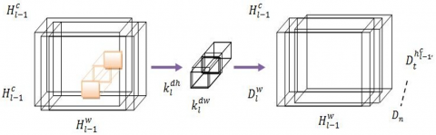
To process inputs, DNN uses a number of convolution layers and then flips the ANN signal on its head. It would be similar to time-domain convolution in classical filtering. This research built a multi-layer DNN on top of each deep filtering subnetwork to guarantee the filter's efficacy. Therefore, it is more accurately described as an evaluation of recoverable convolution operation. By iteratively applying the aforementioned method, the constructed DNN may get representations of supplementary deep structure features. Also, a better component might be indirectly related to all or almost all signals. The deeper unit had more parameters than the deeper unit at a depth, which is a network of separable filters. All of the parameters of the depth-wise separable convolutional filter were generated at random using vessel sound. Data collected from the ship's radiated noise over time might be used to train and fine-tune a separable depth-wise convolution operation's frequency decomposition [28]. Also, a certain wavelength may be associated with a higher-wavelength section of a bigger convolution process, and the converse is also true. The UATR function seems to benefit more from the learnt filtering in this case. A simple 1×1 convolution would suffice for the point-wise inversion, which would then give a linear model of the depth-wise separable level's output. The selected features for training are constructed using an L-number of DWS Region-based Convolutional Neural Network (RCNN) blocks. In the lth DWS RCNN block, the pre-results blocks are used as input. In the $n l-1 h$ and $n l-1 w$ blocks, the channel amount, length, and width were acquired by the $l$-1th DWS RCNN convolution block. When the ship's input audio is represented by $n 0=a$, then $n 0 c=1, \boldsymbol{T} 0 h=1,$ and $\boldsymbol{T} 0 w=N$. The output of the $u$th DWS RCNN convolution block is $\mathbf{b} l c$, where $\mathbf{b} l c, \mathbf{b} l h$, and $\mathbf{b} l w$ are the channel amount and width results. Another way to express the depth-wise convolution that uses a filter for each input channel is as follows:
$D_{t}^{h_{l-1}^{c},d_{l}^{h},d_{l}^{h}}=\left( H_{l-1}^{h_{l-1}^{c}}\times k_{l}^{h_{l-1}^{c}} \right)\left( d_{l}^{h},d_{l}^{w} \right)$ (10)
In Figure 4, we can see the initial step of the suggested system, which is DWS RCNN convolution. The activation function of ReLU is then fed Dl after Batch Normalisation (BN). As shown in Figure 5, the second phase's procedure is described.
Figure 4. The initial stage of a depth-wise method of the proposed system
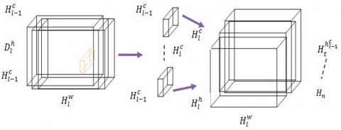
In Figure 4, we can see the initial step of the suggested system, which is DWS RCNN convolution. The activation function of ReLU is then fed Dl after Batch Normalisation (BN). As shown in Figure 5, the second phase's procedure is described.
$D_{l}^{'}=ReLU\left( BN\left( {{D}_{t}} \right) \right)$ (11)
Figure 5. The depth-wise separated compression process in Phase 2
3.4 Modeling assessment
This research employs F1 score and accuracy as markers to assess the proposed approach using actual datasets from commercial boats. Furthermore, this research compares the characteristics that were recovered on their own with those that were purposefully generated using the APRCNN that was suggested. Waveforms, wavelets, HHT, MFCC, Mel frequencies, spectra, cepstrum, non-linear auditory characteristics, and so on are all examples of features that were intentionally manufactured. Also, the histogram and NGS showed how efficient the suggested approach was for clustering. We tested the suggested model using the MXNET DL architecture.
3.5 Data pre-processing
Next, for the rest, there's UAVDT, or unmanned aerial vehicle detection and tracking. Compared to the UAV Mosaicking and Change Detection (UMCD) Dataset, the object detection problem in these two datasets is easier. Much of the imagery appears to have been shot with a conventional isometric lens. Well analyzers will have a somewhat simpler time locating them because of this. This finding proves that the suggested prediction model is the only one capable of identifying the image's components.
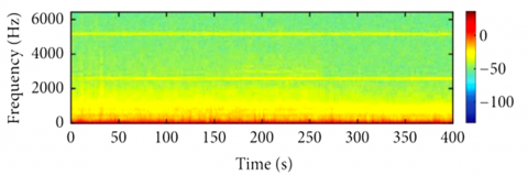
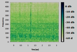
The experimental investigation is based on the original dataset from the actual civil ship. You may find both big and small ships in the collection, as well as ferries. The data is captured at a rate of 48,000 hertz at the anchoring sites. Eighty percent of each class's data is fed into the study's learning algorithm, while twenty percent serves as the test dataset. Underwater noise is depicted in Figure 6 in both the temporal and frequency domains. Figure 7 displays a frequency domain depiction of undersea sound. The colour grade is represented by microvolts, an energy unit.
Figure 6. Underwater audio time domain plot
Figure 7. Underwater noise, spatial frequency
Each track now has its own WAV audio file. The recordings are divided into two parts: a training set and a test set. In the training set, 80% of the instances from each category are used, while in the test set, the remaining 20% are used. There is a 10-second audio segment in every recording, and there are 45-millisecond skips in the input sample and 12.5-millisecond stops in the output sample. Since the training and testing of the network were conducted using real-time data, no pre-processing is required. Table 1 displays the assessment and training data for each class, including the total duration and number of samples.
Table 1. Dataset training and testing
|
Dataset |
Class |
Number of Segments |
Total Time |
Number of Samples |
Percentage (%) |
|
Training |
Small ship Ferry Big ship |
327 561 120 |
0.92 1.56 0.34 |
260742 447746 95234 |
26.2 44.7 9.6 |
|
Testing |
Small ship Ferry Big ship |
83 140 31 |
0.24 0.40 0.09 |
65235 111941 23862 |
26.6 11.2 2.5 |
Table 1 shows that there is a considerable variation in the sample sizes for each class. As an illustration, although small ships constitute 55.7% of the overall random sample, which is over half of the whole random sample, the sample for huge ships would only be 11.9% representative. The sample size is greatly affected by the statistical distribution of each category. This would suggest that, when evaluating several samples for classification, classification performance, rather than accuracy, is the more meaningful metric to use. Therefore, it is necessary to evaluate the proposed model and the effectiveness of category identification using many indicators rather than just one. In this study, dependability and F1 scores are used as performance indicators.
3.6 Learning parameters
Table 2 displays the design of the teachable features extractor. The previously described one-dimensional DWS convolution was used to build the technique of picking teachable characteristics. The first layer was a practical one-dimensional standard. Following each convolution, the BN & ReLU Activation is applied [29]. It evaluates DWS's convolution layer in comparison to more traditional convolution layers by comparing its use of point convolution, BN, and ReLU activation function.
Table 2. Features extraction structure
|
Type |
Stride |
Filter Shape |
Input Size |
|
Conv1D Conv1D dw Conv1D Conv1D dw Conv1D |
51 3 1 1 1 |
204×1×64 dw 12×64 1×1×64×128 15×128 dw 1×1×128×100 |
2176×1 40×64 15×64 15×128 1×100 |
The spatial resolution of the characteristic extraction networks was reduced to 1 when the depth wise and pointwise convolution were treated as separate layers. In networks that extract functionality, there are five tiers. The fundamental model structure can do eleven intensive convolution calculations using an optimized GEMM approach. Before moving the basic convolution to GEMM, a storage classification named "im2col" was necessary. The well-known Caffe package uses this approach, for instance. Instantaneous 1 to -1 convolution might be achieved using GEMM without the need to construct a new storage ranking. Thus, GEMM was the most appropriate tool for dealing with mathematical issues.
3.7 Architecture of time-dilated RCNN
Using the language model as inspiration, Table 3 displays a design of time-dilated convolution layers. A language model informed the construction of a time-dilated convolutional network, which takes as input a two-dimensional matrix $\mathrm{I} \in$ $\mathrm{RT} \times \mathrm{F}$ that is mixed by $\mathrm{T}$ amount of $\mathrm{H}^{\prime}$ and $\mathrm{I}$. The teachable feature extractor generates the one-dimensional underwater acoustic feature set $\mathrm{HH}^{\prime} \in \mathrm{RF}$ at a constant $\mathrm{T}$ time. In this work, the time-dilated convolution has a $\pi\ \mathrm{h}=12$ dilation ratio and exclusively dilates on the time dimension. Every convolution operation uses the BN & ReLU activation functions, however there is no non-linear activation in the convolution itself. Before final max-pooling for classification, the softmax layer receives it. There are five tiers to the timedilated offer comprehensive.
The efficacy of the suggested method was evaluated in this study using the F1 score and reliability. A one-dimensional depth-wise separable inversion network without time-dilated convolution, the proposed APRCNN is compared to a modelling approach with fake construct characteristics in this study. The suggested models' hyper-parameters are displayed in Table 4.
Table 3. Structure of time-dilated RCNN
|
Type |
Stride |
Dilation |
Filter Shape |
Input Size |
|
Conv2D dilation |
1×1 |
12×1 |
3×3×1×64 |
800×100×1 |
|
Max pool |
2×2 |
1×1 |
Pool 2×2 |
777×98×64 |
|
Conv2D dilation |
1×1 |
12×1 |
3×3×64×128 |
388×49×64 |
|
Max pool |
2×2 |
1×1 |
Pool 2×2 |
364×47×128 |
|
Conv2D dilation |
1×1 |
12×1 |
3×3×128×256 |
182×23×128 |
|
Avg pool |
2×2 |
1×1 |
Pool 2×2 |
158×21×256 |
Table 4. The proposed model's hyper-parameters
|
Parameters |
Values |
|
Learning Rate Batch size Epochs Optimizer |
0.001 800 100 RMSprop |
Partially, the system uses APRCNN to mimic the hearing program's spectrum identification and decomposition. Because overfitting on smaller scales can be challenging, this work proposes an alternative to large-scale model retraining that makes use of fewer regularization and information processing strategies. Data from the ship's radiated sound in the time domain was used to train all of the APRCNN's variables. It is also possible to train and tweak the APRCNN's spectrum reduction and observational skills. It is possible that the formation of the mind is reflected in this frequency detection and breakdown.
Images from the testing dataset are selected at random for evaluation, and Figure 8(a-d) displays the corresponding test results. Figure 8 shows its undeveloped terrain with distinct experimental samples. The photos taken underwater and Figure 8(a) The positional accuracy of the identification is shown in the brackets of Figure 8(c), which displays the measurements of (0.882), (0.911), and (0.901) for pictures in that order. Figure 8(b) displays the results of its updated calculation testing. From start to finish, the chosen photographs numbered 4 to 6 were underwater shots. The results of (0.892), (0.931), and (0.937) for 10-12 photos are shown in Figure 8(d) in descending order, with the high accuracy of the identification indicated in brackets. The optimal cat postures for jumping and manoeuvring were shown in the final three acts of Figure 8(a & b) while looking at the randomly selected testing data. Figures 8(c & d) and 2(e) are for underwater motions. Using VGGNet, this system failed to recognize the image's actions. In Figure 8(b) it is visualized. While using the same picture and behavior, this improved approach more accurately recognizes the three samples and produces more accurate internal image movements than its predecessor. Both the accuracy and efficiency of behavior identification in the sample testing images are enhanced by this optimization technique when contrasted with the related approaches.
Figure 8. (a & b) Original imaged (c & d) APRCNN image
Although studying and playing musical instruments have a relatively smaller identification impact compared to other activities, the enhanced APRCNN algorithms evaluate responses on the three techniques of computing, horseback riding, and cycling more extensively. Nevertheless, there has been a significant improvement in the accuracy of location and categorization identification compared to the first algorithms. With a total classification efficiency of 84.7 percent and a location accuracy of 84.7 percent, the new APRCNN computation is useful for computer vision issues in behavioral science, and it also has a much-enhanced identification function.
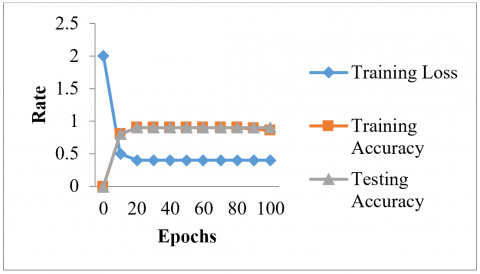
This article utilizes the appropriate time ship scratched random sound for training and modelling testing. A learning group of eight hundred individuals, a potential learning speed of 0.9, and a learning rate from 100 times make up the learning parameters. You can see the whole training programme in Figure 9.
Figure 9. Model training
The development of the model was free of problems with matching, autocorrelation, gradient disappearance, and bursting (Figure 9). The model, which was built using real measurement results, showed impressive detection performance, with a test dataset detection performance of 90.9% and a training data performance of 95.9%. When used to underwater audio data with high levels of noise, the approach obtained a reconnaissance rate of 90.9%. This search yields a discriminating function for the proposed model identification result because, as shown in Figure 10, the sample sizes for each class differ substantially. The contingency table provides more details; on one line, you can see the chosen option, and on the other lines, you can see the actual labels.
Figure 10. The proposed system confusion matrix
There appeared to be high degree of consistency in recognition, as the same outcome was constant across classes (Figure 10). For data sets that are imbalanced in multi-classification concerns, the most popular indicator is the multi-classification F1 score. In a binary classifier, each group assigns a positive score to one class and negative scores to the others. After then, you might use one of these ways to get the grand total of your F1 score. An F1 score that is not weighted is calculated by taking a "macro average." It gives equal weight to all categories, even when the samples are big. The assessment for classification included this data. If all samples were handled equally, the "medium" score would be recommended; if all categories were treated equally, the "medium macro" would be the recommendation. In accordance with the details provided in Table 5, this research determines the groups' accuracy, memory, and F1 score:
Table 5. Performance measures
|
Classes |
Recall |
Support |
F1 Score |
Precision |
|
Small ship Ferry Big ship |
0.92 0.93 0.84 |
65185 111934 23863 |
0.92 0.04 0.82 |
0.92 0.95 0.77 |
|
Accuracy Macro avg Weighted |
0.88 0.92 |
6.6 11.2 2.5 |
0.92 0.89 0.92 |
0.88 0.92 |
Table 5 proves that the model is very accurate and dependable for classifications, as indicated by its high F1 score. The small boats and ferries performed the best, with F1 scores of 0.92 and 0.93, respectively. Recall is 0.84, F1 is 0.82, and dependability is 0.77 for the massive boat on a regular basis. The ferry might be sampling at the same time as some very small vessels, which could explain the phenomenon, or these vessels could share mechanical systems with the ferry. It is defined as the proportion of auditory events that produce classification outcomes. The average accuracy of the comparison models and the suggested designer's model is displayed in Table 6.
Table 6. The proposed model's & comparative models’ classification performance
|
Type |
Method |
Accuracy |
|
Hos |
SVM |
85.1 |
|
Waveform |
SVM |
78.9 |
|
Wavelet |
SVM |
84.3 |
|
Raw time data |
DNN |
88.4 |
|
Raw time data |
DNN |
98.4 |
Analysis of the characteristics collected from the model would follow. In this scenario, we built a distribution for each attribute to find out how often data pieces with that attribute fall within a certain range. Two scatterplots, one for each image, display the feature predominance in each category and the other for the most clearly identifiable traits. Most of the histogram's elements overlap when there is no information or substance. Furthermore, it appears that certain traits have a very high informative character, perhaps as a result of the low overlap in distribution. Underwater sound targets have their 100-dimensional characteristics retrieved in this research. In Figure 11, you can see a couple of feature histograms that the algorithm generated.
Figure 11 shows that some lines have a significantly greater information density and a marked difference for each class. The success of the characteristic extraction is demonstrated by this. Better visualisation and, by extension, a more intricate mapping, are benefits of the algorithmic programme and collector learning. It appears that the t-SNE technology is quite beneficial in this respect. The characteristics of an underwater acoustic target can be better seen with its help. The 100-item characteristic scatter plot is displayed in Figure 12.
Figure 11. The histogram of the characteristics found using the proposed approach
The placement of each group is denoted in Figure 12 by using the corresponding class number. All of the classes were kept apart from one another. The visualisation clearly demonstrates that the features retrieved for the underwater sound lens were highly distinct and consistent, indicating that the model characteristics have great clustering quality. This study uses acquired characteristic charts to build a dataset for underwater audio targets with an identification rate of 98.4 percent. As a result, it appears that feature extraction is mostly responsible for the model's object recognition accuracy, and good feature extraction simplifies design.
Figure 12. A scatter diagram of the identified properties using the proposed model
Using the acquired characteristic charts, this study builds a dataset for underwater audio targets with an identification rate of 98.4 percent. All ships beyond a radius of 5 km (3.1 mi) from the hydrophone were absent while the background noise data for this investigation were collected. Sample rates of 32 kHz are used for background, freight, and passenger data. The overall duration of the data sets used for this experiment is 21.7 hours. The training session lasts for 13.7 hours, and the test for 8 hours. In this study, the data was separated into two sets: the training set and the testing set. This research split the data sets into a training set and a test set. The data was divided into three separate seconds. See the total number of specimens in Table 7. Because the original proportions were too big and worthless, the researchers managed to compress the ship's sound to a smaller one. A spectrogram with one fewer dimension is employed by the researchers. The information spectrum analyzer is shown in Figure 13.
(a)
(b)
(c)
Figure 13. Spectrogram for (a) freight (b) background noise (c) passengers
Table 7. Dataset size (sample)
|
|
Samples Trained |
Samples Tested |
|
Cargo Background Noise Passenger Total |
5976 6296 4293 16421 |
3457 3173 3059 9685 |
The proposed approach achieves the maximum average precision of 90%, as Table 8 shows that this network outperforms the DLMN and DAE comparisons. In contrast, the classification accuracy rate of the DAE system in question is 79%. When it came time to extract sequencing data and distinctive traits from undersea communication targets, as shown by the built DLMN shown7% accuracy over the DAE network. With a 4% improvement in accuracy over the DLMN network, the suggested method proves that the DAE network design can autonomously do away with superfluous speckle noise. The DLMN collaboration network's last fully connected layer generates results that may be used as representations that have been learnt. The visualisation approach is employed to assess the classification performance of t-distributed random neighbourhood features. Figure 14 displays the results. Throughout its existence, the suggested model's characteristics have been the most extensively classified.
Table 8. Classifier outcomes
|
Class |
Recognition Accuracy |
||
|
DAE |
DLSTM |
Proposed Method |
|
|
Background Noise Cargo Passenger Average |
0.89 0.74 0.78 0.80 |
0.91 0.85 0.84 0.87 |
0.96 0.89 0.90 0.91 |
Figure 14. Result of t-SNE feature visualization
Table 9. Performance measures the comparison of existing and proposed systems
|
Methods |
Recall |
Accuracy |
F1 Score |
Precision |
|
CNN RNN GAN |
0.92 0.93 0.84 |
0.92 0.95 0.68 |
0.92 0.04 0.82 |
0.92 0.95 0.77 |
|
RNN LSTM Proposed Method |
0.88 0.92 0.98 |
0.83 0.91 0.99 |
0.92 0.89 0.98 |
0.88 0.92 0.97 |
Figure 15. Comparison of the ROC curve
Receiver Operating Characteristic (ROC) graphs may be constructed using the output of the softmax layer on the training dataset. From a list of three, choose two targets at a time, knowing that one category is beneficial and the other is harmful. In Figure 15, we can see the ROC curves and Areas under the Curve (AUC) tests that were conducted using different approaches. Compared to competing methods, the suggested model outperforms them in almost every category. Table 9 details the performance metrics used to compare the suggested system to other DNN models already in use.
By optimising the APRCNN model parameters driven by time-domain vessel noise, this work aims to alleviate the UATR problem. The deeper features of the underwater acoustic target, as retrieved by the proposed approach, seem to be quite stable and easily separable. A database with the real audio energy of civilian ships was used to test the classification, and it obtained an average recognition rate of 98.4%. Despite a high rate of identification, actual enforcement is inadequate, therefore there is space for development. The testing results further demonstrate that the submerged object's 100-dimensional properties were stable and easy to distinguish. In this study, we provide a new collaborative deep-learning approach to underwater audio target identification. The proposed method combines DLMN and DAE neural networks into a single model to achieve optimal performance. In terms of classification, the experimental results reveal that the proposed technique outperforms the DAE and DLMN neural networks. Future research will focus on enhancing the UATR's performance metric.
[1] Zhang, W., Yang, X., Leng, C., Wang, J., Mao, S. (2022). Modulation recognition of underwater acoustic signals using deep hybrid neural networks. IEEE Transactions on Wireless Communications, 21(8): 5977-5988. https://doi.org/10.1109/TWC.2022.3144608
[2] Feng, S., Zhu, X. (2022). A transformer-based deep learning network for underwater acoustic target recognition. IEEE Geoscience and Remote Sensing Letters, 19: 1-5. https://doi.org/10.1109/LGRS.2022.3201396
[3] Zhang, Y., Zhu, J., Wang, H., Shen, X., Wang, B., Dong, Y. (2022). Deep reinforcement learning-based adaptive modulation for underwater acoustic communication with outdated channel state information. Remote Sensing, 14(16): 3947. https://doi.org/10.3390/rs14163947
[4] Jiang, J., Wu, Z., Huang, M., Xiao, Z. (2022). Detection of underwater acoustic target using beamforming and neural network in shallow water. Applied Acoustics, 189: 108626. https://doi.org/10.1016/j.apacoust.2021.108626
[5] Anand, M., Balaji, N., Bharathiraja, N., Antonidoss, A. (2021). WITHDRAWN: A controlled framework for reliable multicast routing protocol in mobile ad hoc network. Materials Today: Proceedings. https://doi.org/10.1016/j.matpr.2020.10.902
[6] Lv, Z., Du, L., Li, H., Wang, L., Qin, J., Yang, M., Ren, C. (2022). Influence of temporal and spatial fluctuations of the Shallow Sea acoustic field on underwater acoustic communication. Sensors, 22(15): 5795. https://doi.org/10.3390/s22155795
[7] Li, Y., Tang, B., Geng, B., Jiao, S. (2022). Fractional order fuzzy dispersion entropy and its application in bearing fault diagnosis. Fractal and Fractional, 6(10): 544. https://doi.org/10.3390/fractalfract6100544
[8] Li, Y., Jiao, S., Geng, B. (2023). Refined composite multiscale fluctuation-based dispersion Lempel–Ziv complexity for signal analysis. ISA Transactions, 133: 273-284. https://doi.org/10.1016/j.isatra.2022.06.040
[9] Li, Y., Geng, B., Tang, B. (2023). Simplified coded dispersion entropy: A nonlinear metric for signal analysis. Nonlinear Dynamics, 111(10): 9327-9344. https://doi.org/10.1007/s11071-023-08339-4
[10] Joby, P.P. (2022). An extensive research on acoustic underwater wireless sensor networks (AUWSN). IRO Journal on Sustainable Wireless Systems, 4(2): 121-129. https://doi.org/10.36548/jsws.2022.2.006
[11] Lucas, E., Wang, Z. (2022). Performance prediction of underwater acoustic communications based on channel impulse responses. Applied Sciences, 12(3): 1086. https://doi.org/10.3390/app12031086
[12] Wu, S.S., Anjangi, P., Chitre, M. (2022). Adaptive modulation and feedback strategy for an underwater acoustic link. In 2022 Sixth Underwater Communications and Networking Conference (UComms), Lerici, Italy, pp. 1-5. https://doi.org/10.1109/UComms56954.2022.9905694
[13] Deeraj, P., Rohit, G., Abhishek, K.S., Subashka, S.S. (2020). A trash barrel suitable for both indoor and outdoor uses (A better way to clean your garbage). International Journal of Advanced Science and Technology, 29(5): 3103-3110.
[14] Han, X.C., Ren, C., Wang, L., Bai, Y. (2022). Underwater acoustic target recognition method based on a joint neural network. Plos One, 17(4): e0266425. https://doi.org/10.1371/journal.pone.0266425
[15] Latchoumi, T.P., Ezhilarasi, T.P., Balamurugan, K. (2019). Bio-inspired weighed quantum particle swarm optimization and smooth support vector machine ensembles for identification of abnormalities in medical data. SN Applied Sciences, 1(10): 1137. https://doi.org/10.1007/s42452-019-1179-8
[16] Zhang, Y., Li, C., Wang, H., Wang, J., Yang, F., Meriaudeau, F. (2022). DL-aided OFDM receiver for underwater acoustic communications. Applied Acoustics, 187: 108515. https://doi.org/10.1016/j.apacoust.2021.108515
[17] Zhang, Y., Wang, H., Li, C., Chen, X., Meriaudeau, F. (2022). On the performance of deep neural network aided channel estimation for underwater acoustic OFDM communications. Ocean Engineering, 259: 111518. https://doi.org/10.1016/j.oceaneng.2022.111518
[18] Chen, L., Liu, F., Li, D., Shen, T., Zhao, D. (2022). Underwater acoustic target classification with joint learning framework and data augmentation. In 2022 5th International Conference on Artificial Intelligence and Big Data (ICAIBD), Chengdu, China, pp. 23-28. https://doi.org/10.1109/ICAIBD55127.2022.9820117
[19] Subashka Ramesh, S.S., Hassan, N., Khandelwal, A., Kaustoob, R., Gupta, S. (2019). Analytics and machine learning approaches to generate insights for different sports. International Journal of Recent Technology and Engineering, 7(6): 1612-1617.
[20] Yaman, O., Tuncer, T. (2023). Accurate deep and direction classification model based on the antiprism graph pattern feature generator using underwater acoustic for defense system. Multimedia Tools and Applications, 82(7): 9961-9985. https://doi.org/10.1007/s11042-022-13196-1
[21] Xiao, W., Luo, Z., Hu, Q. (2022). A review of research on signal modulation recognition based on deep learning. Electronics, 11(17): 2764. https://doi.org/10.3390/electronics11172764
[22] Huang, Z., Li, S., Yang, X., Wang, J. (2022). OAE-EEKNN: An accurate and efficient automatic modulation recognition method for underwater acoustic signals. IEEE Signal Processing Letters, 29: 518-522. https://doi.org/10.1109/LSP.2022.3145329
[23] Garikapati, P., Balamurugan, K., Latchoumi, T.P., Malkapuram, R. (2021). A cluster-profile comparative study on machining AlSi7/63% of SiC hybrid composite using agglomerative hierarchical clustering and K-means. Silicon, 13(4): 961-972. https://doi.org/10.1007/s12633-020-00447-9
[24] Rahman, M.H., Sejan, M.A.S., Yoo, S.G., Kim, M.A., You, Y.H., Song, H.K. (2022). Multi-user joint detection using bi-directional deep neural network framework in NOMA-OFDM system. Sensors, 22(18): 6994. https://doi.org/10.3390/s22186994
[25] Zhang, Y., Wang, H., Li, C., Meriaudeau, F. (2022). Data augmentation aided complex-valued network for channel estimation in underwater acoustic orthogonal frequency division multiplexing system. The Journal of the Acoustical Society of America, 151(6): 4150-4164. https://doi.org/10.1121/10.0011674
[26] Umamageswari, A., Bharathiraja, N., Irene, D.S. (2023). A novel fuzzy C-means based chameleon swarm algorithm for segmentation and progressive neural architecture search for plant disease classification. ICT Express, 9(2): 160-167. https://doi.org/10.1016/j.icte.2021.08.019
[27] Gao, D., Hua, W., Su, W., Xu, Z., Chen, K. (2022). Supervised contrastive learning-based modulation classification of underwater acoustic communication. Wireless Communications and Mobile Computing, 2022: 3995331. https://doi.org/10.1155/2022/3995331
[28] Zhang, W., Lin, B., Yan, Y., Zhou, A., Ye, Y., Zhu, X. (2022). Multi-features fusion for underwater acoustic target recognition based on convolution recurrent neural networks. In 2022 8th International Conference on Big Data and Information Analytics (BigDIA), Guiyang, China, pp. 342-346. https://doi.org/10.1109/BigDIA56350.2022.9874151
[29] Ashok, P., Latha, B. (2023). Absorption of echo signal for underwater acoustic signal target system using hybrid of ensemble empirical mode with machine learning techniques. Multimedia Tools and Applications, 82(30): 47291-47311. https://doi.org/10.1007/s11042-023-15543-2