Pallavi Srivastava*![]() | Aasheesh Shukla
| Aasheesh Shukla![]() | Atul Bansal
| Atul Bansal![]()
© 2024 The authors. This article is published by IIETA and is licensed under the CC BY 4.0 license (http://creativecommons.org/licenses/by/4.0/).
OPEN ACCESS
Soil organic matter (SOM) and soil moisture content (SMC) are critical indicators of soil health, yet their measurement using conventional methods is often prohibitive due to high time, labor, and financial costs. To address these challenges, a novel model employing image processing techniques has been developed to predict SOM and SMC based on soil colour features. This model utilizes stepwise multiple linear regression (SMLR) to correlate soil colour attributes, such as colour moments, Gray Level Co-occurrence Matrices (GLCMs), and various colour models, with the moisture and organic content of the soil. Field samples were systematically collected at defined intervals to represent continuous variation in soil properties. The ground truth for model calibration was established using the loss of ignition method. The efficacy of the model was validated externally, with the selection of 34 initial and then 6 optimal predictor variables, yielding an R2 of 0.67 and a Root Mean Square Error (RMSE) of 0.76 for SOM prediction, and an R2 of 0.77, RMSE of 0.55, and a Ratio of Performance to Inter-Quartile (RPIQ) of 1.07 for SMC. These results demonstrate the potential of using image-based modeling as a robust tool for soil property analysis.
predictive analysis, soil moisture content (SMC), step-wise linear regression, soil organic matter (SOM), cubist, Vtreat, ANOVA, computer vision, soil colour
For human beings, images are one of the best sources of information because they support deeply understanding any kind of scene. With that influence, scientists and researchers have attempted to utilize this quality visual information in different applications. Image processing involves synthesizing the images using computers. As a result, images are an enormous source of information that can be used if their features are properly examined. For getting different kinds of results, there are different processes, namely, image restoration, image compression, image enhancement, image registration, etc. For the last many years, the agriculture field has found many applications using image processing and machine learning. Some of the applications are fruit grading [1], precision farming [2], weed detection [3], crop prediction [4], soil texture classification and prediction [5], soil pH level prediction [6], etc.
One of the streaming applications is SMC and SOM prediction [7]. SOM is an essential component of high-quality and healthy soil. It is comprised of organic remains from animals and plants along with material converted by microorganisms present in the soil at various decomposition stages. This shows an effect on agriculture and forestry production. Good-quality soils with steady levels of organic matter are capable of preventing and fighting soil-borne diseases. Moreover, SOM has a key role in boosting soil quality and fertility. SOM gives an idea of the extent of nitrogen supply that soil can provide for determining crop growth. Although organic matter varies greatly on the surface within the field [7], these spatial SOM statistics help to decide the management of site-wise agricultural resources, which involves applying nitrogen fertilizer and achieving a trade-off between environmental pollution reduction and crop production increase [8], which is one of the important components of precision agriculture [9]. SMC is the quantity of water present in soil. It is one of the most important soil properties and has many advantages associated with knowing the amount of moisture present in it, such as the measure of the need for irrigation, the availability of nutrients and chemicals, erosion, biological activity, and compaction potential. Thus, knowing the properties of soils like SOM and SMC has an association with the health of the soil. So, it helps farmers and land managers make decisions to enhance soil conditions. Some of the challenges in estimating and assessing SOM and SMC are labor and time-exhaustive laboratory evaluation [10], supervising variability in SMC and SOM [11], diversification in space [12], and the effectiveness of component-like types of soil [13, 14].
The above-mentioned challenges have made the researchers conscious of developing and generating cost-effective and rapid ways to estimate soil properties. Soil colour is one of the most result-oriented characteristics in determining soil properties. Soil colour has also been used in soil identification [15]. It is a feature that has been observed to have a strong correlation with spectral reflectance features and between SOM and soil colour [16-21] and SMC and soil colour [22-25]. The dark colour of the soil is essentially linked to higher values of SOM, SMC, and intrinsic soil fertility [26-28]. Therefore, this kind of content comes through modeling.
Existing research work on image processing-based SOC and SOM predictions [29-33] has soil colour as a main link. Dark soil colour is usually associated with high contents of organic matter; this kind of soil is fertile and capable of supporting plant growth [19]. The Munsell colorimetric system [34] is a conventional method for quantifying soil colour, which involves subjective visual matching between standard colour chips and soil samples. Therefore, when accurate colour dynamics and automatic colour matching are required, the Munsell colorimetric system is a suitable method. Modern image acquisition devices have control over the drawbacks of the Munsell colorimetric system and enhance SOM predictions. In some of the research work [30], a NIR high-resolution digital camera with controlled conditions was used for SOM prediction. It was stated that SOM was associated with the intensity of all the wavebands. It was observed that the CIEL*c*h* and CIEL*u*v* models were a good fit for SOC prediction [31]. A later study [32] predicted SOC in a comparative format by using different colour spaces. Other various studies also considered a stronger relationship between the colour of the soil sample and SOM [30, 31, 35-38]. Later, this relationship was tested on the cell-phone application SOCIT [39].
In many studies [29, 32, 39, 40], for SOM prediction, a prime parameter used is soil colour in order to develop a prediction model, but with no intention of using other factors like surface residue, soil moisture, or surface roughness [41]. Out of all such factors, SMC is an important factor that controls the practical assessment of SOM. Generally, wet soils [42, 43] are darker in colour than dry soils. Soil macro- and micropores slowly permeate with water, which changes the physical composition of the soil with an increase in SMC. As a consequence, the relative refractivity of soil particles [14] changes, which causes a change in soil colour. This in turn complicates the relationship between soil colour and SOM, which becomes one of the deciding factors for predicting SOM from images. In the above-mentioned studies, SMC was an absolute factor in predictive models as soil samples have a variable value of moisture content. Furthermore, some of the research work introduced the concept of finding a moisture content, which is a SMC threshold value. The values below or above this threshold have different soil colours [14, 29]. Many reasons contribute to the decision about the value of the SMC threshold. Few researchers also observed soil reflectance as a change in the visible region only until SMC reaches 20% [44-47]. A study suggested a critical SMC of 15% [14]. There are some proofs of the critical value of the SMC influencing the soil reflectance and the way it can impact the SOM prediction using digital images.
The objective of this study was to predict SMC and SOM using colour and textural features extracted from soil sample images (Figure 1). This paper evaluates the ability of soil sample images acquired from a smartphone camera. The models are calibrated and validated for developing predictive analyses between features extracted from images and laboratory-measured SMC and SOM. Additionally, a few best-performing features are also sorted out of all the features. Figure 2 shows the overall workflow in the form of a block diagram.
Figure 1. Few examples of soil sample dataset
Figure 2. Proposed model for SOM and SMC prediction
A set of 250 soil samples was considered in this study. These consist of samples from five different crops: potato, sugarcane, mustard, wheat, and rice. The sample collection site is located at 25°56'30"N latitude and 83°33'40"E longitude. These samples were collected from the district Mau, Uttar Pradesh, India. For every crop, 10 fields of approximately the same size are considered. Five samples of soil are dug out of 10 fields. So, 250 soil samples comprising all five crops were captured. Multiple samples were considered from multiple fields as the fields demonstrated high spatial (within the field) variations [48] in SOM and SMC. A large number of soil samples constitute the variation in soil conditions precisely; here, 250 soil samples were collected, representing a broad variation in organic matter content (2.5-74.6%). These samples are dug out from a depth of 2 inches below the surface of the field. These samples were uniformly taken out on a white sheet for image acquisition. Images (3024×4032 pixels) were captured with a 16-megapixel smartphone camera. The device was kept 20 inches above the surface of the soil sample. The camera settings are kept in default conditions, such as exposure time = 1/30s, F-stop = f/1.8, focal length = 1.12, and images were saved as a joint photographic experts group (JPEG). At the time of creating the soil image dataset, 8 images of each sample were captured. Therefore, there are a total 2000 soil images in the dataset. Figure 1 shows some examples of the soil sample images from the dataset.
In this study, SMC was consistently maintained during laboratory experiments, similar to other studies [49], despite its quasi-normal distribution in field observations [8]. The SMC and SOM were measured using the loss on ignition (LOI) method [48]. Maintaining constant SMC in samples can introduce bias in feature extraction through image processing, as different soil samples vary not only in SOM but also in water holding capacity. For instance, a sample with 2.59% SOM registered an SMC of 25.51%, whereas a sample with 6.91% SOM showed an SMC of 53.47%. Figure 2 outlines the methodological steps followed: initially, soil samples are collected and the ground truth is established; subsequently, illumination normalization is applied to the images; features are then extracted for various colour models; finally, a regression model is assessed using diverse output parameters.
3.1 Segmentation of region of interest
Before providing images to any feature extraction network, the soil images are first segmented to generate the region of interest. For this purpose, two different methods are applied: the threshold method and Otsu’s method. First, the threshold method is used to segment the image. Figure 3 shows the outcome of applying different values of thresholds. It is clear from this image that the method operates best at a threshold value of 0.50. It shows that the selected threshold value is best according to the fraction of pixels. The histogram from Figure 4 clearly shows why the optimal threshold value is in the range of 0.40 to 0.60.
After this, Otsu’s method is used to segment the region of interest from the image. It is a better solution than determining the best threshold value by binarizing the image. However, this method relies on the fact that the image consistently consists of a background and a foreground, indicating that the histogram should clearly show only two separable distributions. Figure 5 shows the outcome of Otsu’s method. Though the result of this method performs the task of segmentation, certain areas in the region of interest are predicted as background. As can be observed from the segmentation results, the threshold method generated better segmentation results than Otsu’s method. So, further image processing analysis is performed on the output images of the threshold method.
Figure 3. Result of threshold segmentation method
Figure 4. Histogram for optimal value of threshold
Figure 5. Result of Otsu’s segmentation method
3.2 Illumination normalization
In the soil image dataset, there can be illumination variation in the images due to changes in lighting, shadows, noise, and also because the images were captured on different days. Illumination normalization was performed by dividing every pixel of the segmented region of interest in soil images by the mean value of the intensity of its corresponding reference, as shown in Eq. (1):
$N(a, b)_{I \lambda}=N(a, b)_{O \lambda} / \operatorname{MeanN}(a, b)_{R \lambda}$ (1)
where, $N(a, b)_{O \lambda}=$ original pixel value at the ath row and bth column of soil ROI; $N(a, b)_{o \lambda}=$ Illumination normalized pixel value at the ath row and bth column of soil ROI; $\operatorname{MeanN}(a, b)_{R \lambda}=$ Mean pixel of the corresponding reference for specific waveband $\lambda$. As a suggestion for future work, a band or a colour pallet can be used as a reference for illumination normalization.
3.3 Feature extraction
After segmentation and illumination normalization, feature extraction is carried out. At the time of storing soil images, the colour space was RGB with R, G, B as the primary colour parameters. Afterwards, images were transformed into different colour models with multiple or secondary colour metrics with different information levels. In this proposed work, 34 different features were extracted, including colour features. Sample images were acquired and stored in RGB colour space. For this step, the images were converted to other colour spaces, including HSV, YIQ, YCbCr, CIEL*a*b. Along with these colour moments, a gray co-occurrence matrix was also calculated. 34 features, including median R, G, B, H, S and V, mean R, G, B, H, S, V, mean gray, median gray, homogeneity, contrast, and energy were taken into account. These features have mean and median of different colour spaces. Table 1 shows the definition of these features.
Table 1. Description of features extracted from images
|
Feature |
Description |
|
Mean |
Average of values of all pixels in an image |
|
Median |
Middle pixel value after all the pixels is sorted in numerical order |
|
Entropy |
Statistical measure of randomness |
|
Contrast |
Measure of intensity contrast between a pixel and its neighbour over the whole image |
|
Energy |
Sum of squared elements in the gray level co-occurrence matrix (GLCM) |
|
Homogeneity |
Closeness of distribution of elements in the GLCM to the GLCM |
A total of 2000 soil images were captured while acquiring the dataset from soil samples. For result evaluation, the model is analyzed using 10-fold cross-validation. The dataset is divided into calibration and validation with a ratio of 80:20. The Kennard-Stone [50-52] algorithm was used for this data division. Features extracted from images were used to build a predictive relationship to the laboratory-measured SMC and SOM values. The results are verified using internal and external validation. For internal validation, 10-fold cross-validation is used, where data is divided into 80:20 for training and testing. For external validation, leave one out cross-validation (LOOCV), where the model is trained using all the data except one image, which is used for testing. This is repeated until every single image is used for testing. A stepwise multiple linear regression (SMLR) predictive model is developed to use the relation between colour parameters SOM (and also SMC). The SMLR model is also proposed (Figure 2) between colour features and SMC, which includes SOM. At every step of forward SMLR, one of the most statistically significant features with the lowest p-value is added to the model, and accordingly, the variation in p-value and F-statistics is logged. The threshold for the p-value was set at 0.07 to exclude or include a colour feature. Multi-collinearity was taken into consideration as a strong correlation is found between colour features, which can be observed in Table 2. The root mean square error (RMSE) and coefficient of determination (R2) are used to evaluate the model. The subscripts c, v, and cv represent calibration, validation, and LOOCV.
$R M S E_{c v}=\sqrt{\sum_{i=1}^n\left(Y_e-Y_m\right)^2 / n}$ (2)
where, Ye is the predicted SOM; Ym is the measured SOM, and n is the number of samples. RMSEC and RMSEv were calculated by using Eq. (2) too.
$R P D_{C V}=S D / R M S E_{c v}$ (3)
RPDC and RPDV were calculated by using Eq. (3) too. In the study, RPD classification followed Chang et al. [51].
Table 2. SOM and SMC descriptive statistics with soil colour
|
Parameter |
Mean |
SD |
Skewness |
COV(%) |
|
Mean R |
0.45 |
0.22 |
-0.07 |
48.89 |
|
Mean G |
0.42 |
0.21 |
-0.15 |
50.00 |
|
Mean B |
0.40 |
0.20 |
-0.19 |
50.00 |
|
Mean H |
0.20 |
0.13 |
4.08 |
65.00 |
|
Mean S |
0.26 |
0.15 |
0.77 |
57.69 |
|
Mean V |
0.35 |
0.21 |
-0.06 |
60.00 |
|
Mean L* |
0.17 |
0.11 |
0.09 |
62.53 |
|
Mean a* |
0.13 |
0.13 |
-0.14 |
100.62 |
|
Mean b* |
0.16 |
0.17 |
-0.17 |
103.53 |
|
Mean Y |
0.72 |
0.20 |
-0.19 |
27.78 |
|
Mean Cb |
0.52 |
0.21 |
0.42 |
40.38 |
|
Mean Cr |
0.62 |
0.16 |
0.54 |
25.81 |
|
Mean Y |
0.65 |
0.24 |
0.72 |
36.15 |
|
Mean I |
0.17 |
0.21 |
-0.15 |
123.53 |
|
Mean Q |
0.066 |
0.20 |
-0.17 |
30.30 |
|
Median R |
0.48 |
0.24 |
0.24 |
50.00 |
|
Median G |
0.46 |
0.23 |
0.23 |
50.00 |
|
Median B |
0.43 |
0.22 |
0.22 |
50.00 |
|
Median H |
0.20 |
0.10 |
0.15 |
50.00 |
|
Median S |
0.30 |
0.15 |
0.15 |
50.00 |
|
Median V |
0.37 |
0.16 |
0.18 |
43.78 |
|
Median L* |
0.20 |
0.10 |
0.10 |
50.50 |
|
Median a* |
0.17 |
0.15 |
0.08 |
88.23 |
|
Median b* |
0.26 |
0.13 |
0.13 |
50.00 |
|
Median Y |
0.85 |
0.42 |
0.42 |
49.42 |
|
Median Cb |
0.54 |
0.22 |
0.27 |
40.74 |
|
Median Cr |
0.72 |
0.36 |
0.36 |
50.00 |
|
Median Y |
0.68 |
0.35 |
0.34 |
51.47 |
|
Median I |
0.74 |
0.37 |
0.28 |
50.00 |
|
Median Q |
0.075 |
0.032 |
0.034 |
42.67 |
|
Entropy |
5.82 |
0.49 |
-0.82 |
8.42 |
|
Contrast |
3.37 |
3.07 |
3.20 |
91.09 |
|
Energy |
0.42 |
0.41 |
2.80 |
97.62 |
|
Homogeneity |
0.92 |
0.08 |
0.81 |
8.69 |
|
SOM (%) |
21.05 |
19.65 |
2.23 |
93.35 |
|
SMC (%) |
26.07 |
30.12 |
2.01 |
115.53 |
Initially, all 34 features were used to predict SOM (%) and SMC (%) as predictor variables. Internally, 10-fold cross-validation was also performed. The difference between the ground truth and the predicted value was also taken into account. This difference function was found advantageous for pedo-transfer function development. Performance metrics calculated to analyze the model were:
RMSE (Root Mean Square Error);
R2 (coefficient of determination);
Bias (mean of the residuals);
LCCC (Lin’s Concordance Correlation Coefficient);
RPIQ (Ratio of Performance to Interquartile Distance);
RPD (Ratio of Performance to Deviation).
The ratio of the standard deviation of measured values to the standard error of prediction is known as RPD [51]. RPD values greater than 2 indicate that a model is qualitatively good. RPIQ is also calculated because RPD is linked closely to R2 [52]. RPIQ gives a better representation of the spread of values in the dataset. Low values of bias and RMSE, and large values of R2 and LCCC represent higher prediction accuracies.
Z-score was described on top of the performance of each predictor, and four different analysis tests were done, namely, ANOVA (Analysis of Variance), Cubist, Correlation, and Vtreat. Predictors were given a rating in a range of 0 to 100 (with 0 as the least important and 100 as the most important), and then these were averaged to get a z-score. Cubist analysis gives information on variable importance in a range of 0 to 100; results that are not on the same scale are converted to the same range of 0 to 100. The analysis of correlation showed a 1:1 correlation between the dependent variable and each predictor. It had values between 0 (the least important) and 100 (the most important) correlation coefficients. In ANOVA, the p-value for every predictor is calculated between 0 and 100, with 0 being the lowest and 100 being the highest p-value. R2 values are recorded between 0 and 100, with 0 as the lowest value and 100 as the highest value. These values are then added and averaged to generate the scaled values in the described range of 0 to 100; these values are z-scores for a certain predictor. After this, the four highest predictor variables were then identified as the optimum predictors for both SOM and SMC. All this development of the model was again trained on these four predictors as independent variables, and model assessment metrics were calculated.
5.1 Descriptive analysis
Observed descriptive statistics of SOM and SMC have shown a high level of alteration in coefficient of variation, COV (%); the values were between 8.42% and 123.53% for soil properties and image features (Table 2). Values of SOM are observed between 3.45% and 81.50%, with 21.05% as the mean value and 19.65% as the standard deviation. These soil samples are highly variable and were chosen to make sure that the results are versatile. Taking from the high values of SOM, observed SMC values varied between 10.12% and 120.34%, with 26.07% as the mean value and 30.12% as the standard deviation value. Mean I indicated a high value of COV, which is 123.53%. But on the other side, homogeneity was less variable, with a COV of 8.69%.
5.2 Correlation of SMC and SOM with soil colour
The advantages of soil colour were evaluated by examining the relationship between digital measurement of the colour of the soil, SOM, and SMC. Median H is weakly correlated (r = 0.16) to SMC. Median B and SMC are highly correlated (r = - 0.75) to each other which is followed by median V (r = - 0.72) and median Y (r = - 0.70). SOM is strongly correlated with mean H (r = - 0.60), then to energy (r = - 0.57) and mean S (r = - 0.53). The lowest correlation (r = 0.09) of SOM is with entropy. The value correlation was also significant in many cases for both SMC and SOM.
5.3 Predictive analysis
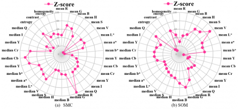
Four different study criteria are presented in radial plots (Figures 6-8) to show the comparative gravity of predictors in predicting SMC and SOM. In many studies, colour features of soil have shown a significant role in the prediction of SOM and SMC in comparison to textural features. Researchers found that colour spaces RGB and HSV were more important in predicting SMC and SOM than other colour spaces. Moreover, median values taken from the channels of colour spaces were more significant while predicting than the mean values. Significant predictors in SMC prediction are Median R and Median Cb, followed by Median Y, Median Cr, Median V, and Mean G. The less significant variable was mean S (Figure 7). In the case of SOM prediction, the most significant variable is Mean V. The least significant variable was Mean S (Figure 8). SMLR was established with 34 and 6 features. It was first calibrated and then validated against the laboratory-measured SOM and SMC. Table 3 and Table 4 present detailed prediction statistics results obtained using 34 and 6 predictor variables.
5.3.1 Prediction of SMC
For predicting SMC, the model was calibrated and validated for 34 (all) predictor variables, and then, using z-score statistics, six optimal predictor variables were finalized. Based on the z-scores from the radial graph presented in Figure 6(a), Median R was identified as the most important variable in predicting SMC, followed by Median Cb, Median Y, Median Cr, Mean G, and Median V. Finally, the model is calibrated and validated for those six predictor variables. Both internal and external validation processes recorded the output metrics for the prediction of SMC. When considering all the features, the R2, LCCC, RMSE, RPD, and RPIQ values were 0.62, 0.67, 7.90%, 2.78, and 1.57, respectively, for 10-fold cross-validation, which is the internal validation. For the test dataset, meaning external validation, R2, LCCC, RMSE, RPD, and RPIQ values were 0.67, 0.55, 7.60%, 1.64, and 1.00, respectively. For six predictor variables with internal validation, the R2, LCCC, RMSE, RPD, and RPIQ values were 0.67, 0.65, 7.50%, 5.56, and 1.79, respectively. For external validation, the R2, LCCC, RMSE, RPD, and RPIQ values were 0.56, 0.56, 6.70%, 1.87, and 1.14, respectively.
5.3.2 Prediction of SOM
The method of predicting SOM follows the same steps as the prediction of SMC: the model was calibrated and validated for 34 (all) predictor variables, and then, using z-score statistics, six optimal predictor variables were finalized. Based on the z-scores from the radial graph presented in Figure 6(b), Mean V was identified as the most important variable in predicting SOM, followed by Median G, Median Q, Mean H, Mean S and Mean L*. Finally, the model is calibrated and validated for those six predictor variables. The output metrics for the prediction of SMC were recorded through internal and external validation processes. When considering all the features, the R2, LCCC, RMSE, RPD, and RPIQ values were 0.75, 0.73, 7.80%, 2.13, and 1.36, respectively. For the test dataset, meaning external validation, R2, LCCC, RMSE, RPD, and RPIQ values were 0.77, 0.75, 5.5%, 1.88, and 1.07, respectively. For six predictor variables with internal validation, the R2, LCCC, RMSE, RPD, and RPIQ values were 0.81, 0.78, 7.3%, 2.11, and 1.57, respectively. For external validation, the R2, LCCC, RMSE, RPD, and RPIQ values were 0.92, 0.85, 4.4%, 1.98, and 1.21, respectively.
Table 3. Prediction accuracy for SMC using 34 and 6 predictor variables. The results are of 10 fold cross validation internal validation (IV) and external validation (EV)
|
Model |
R2 |
LCCC |
RMSE |
RPD |
RPIQ |
|||||
|
IV |
EV |
IV |
EV |
IV |
EV |
IV |
EV |
IV |
EV |
|
|
Using 34 predictor variables |
||||||||||
|
SMLR |
0.62 |
0.67 |
0.67 |
0.55 |
0.79 |
0.76 |
2.78 |
1.64 |
1.57 |
1.00 |
|
Using 6 predictor variables |
||||||||||
|
SMLR |
0.67 |
0.56 |
0.65 |
0.56 |
0.75 |
0.67 |
2.56 |
1.87 |
1.79 |
1.14 |
Table 4. Prediction accuracy for SOM using 34 and 6 predictor variables. The results are of 10 fold cross validation internal validation (IV) and external validation (EV)
|
Model |
R2 |
LCCC |
RMSE |
RPD |
RPIQ |
|||||
|
IV |
EV |
IV |
EV |
IV |
EV |
IV |
EV |
IV |
EV |
|
|
Using 34 predictor variables |
||||||||||
|
SMLR |
0.75 |
0.77 |
0.73 |
0.75 |
0.78 |
0.55 |
2.13 |
1.88 |
1.36 |
1.07 |
|
Using 6 predictor variables |
||||||||||
|
SMLR |
0.81 |
0.92 |
0.78 |
0.85 |
0.73 |
0.44 |
2.11 |
1.98 |
1.57 |
1.21 |
Figure 6. Z-score for features representing the priority towards SMC and SOM prediction
Figure 7. Significance of individual feature as a predictor for SMC prediction corresponding to ANOVA, Cubist, Vtreat, Correlation
Figure 8. Significance of individual feature as a predictor for SOM prediction corresponding to ANOVA, Cubist, Vtreat, Correlation
The performance of the SMLR model was assessed for its effectiveness in providing both reasonable and rapid estimations of SOM and SMC using a dataset acquired in a laboratory setting with a smartphone camera. This cost-effective method utilized a smartphone camera to classify soil properties based on texture and colour features derived from soil images. Experiments involved soil samples from five different crops, reflecting variable organic matter content. Images were captured at various heights to account for continuous changes in both SMC and SOM. Initially, all 34 features were analyzed, followed by a refined selection of 6 optimal features for both SOM and SMC. It was observed that darker soil coloration correlates strongly with higher organic and moisture content. The model underwent both internal and external calibration and validation, with performance metrics recorded for each. While this study includes samples from diverse crop fields exhibiting significant variations in organic matter, future research should explore the impact of SMC variations on soil organic content more thoroughly. Further studies should also investigate the relationship between soil colour and its properties, SMC and SOM, to enhance predictive accuracy. Table 5 shows a comparison of proposed model with existing models.
Table 5. Comparison of existing literature and proposed model
|
Ref. |
Output Algorithms |
Dataset Acquisition Device |
Performance (%) |
|
|
SMC |
SOM |
|||
|
Fu et al. [7] |
Stepwise linear regression |
Cellular phone, 10- megapixel |
- |
R2 = 0.819 RMSE= 7.747% RPD = 2.328 |
|
Wu et al. [37] |
- |
Canon 5D Mark III. camera, 22.3 megapixel |
- |
R2 = 0.52
|
|
Rienzi et al. [46] |
Partial least square regression |
- |
- |
R2 = 0.64 |
|
Proposed model |
Stepwise linear regression |
Motorola one power smartphone |
R2 = 0.67 LCCC = 0.65 RMSE = 7.5% RPD = 5.56 RPIQ = 1.79 |
R2 = 0.81 LCCC = 0.78 RMSE= 7.3% RPD = 2.11 RPIQ = 1.57 |
[1] Bhargava, A., Bansal, A. (2020). Machine learning based quality evaluation of mono-colored apples. Multimed Tools Appl, 79(31): 22989-23006. https://doi.org/10.1007/s11042-020-09036-9
[2] Azizi, A., Abbaspour-Gilandeh, Y., Vannier, E., Dusséaux, R., Mseri-Gundoshmian, T., Moghaddam, H.A. (2020). Semantic segmentation: A modern approach for identifying soil clods in precision farming. Biosystems Engineering, 196: 172-182. https://doi.org/10.1016/j.biosystemseng.2020.05.022
[3] Wu, Z., Chen, Y., Zhao, B., Kang, X., Ding, Y. (2021). Review of weed detection methods based on computer vision. Sensors, 21(11). https://doi.org/10.3390/s21113647
[4] Honawad, S.K., Chinchali, S.S., Pawar, K., Deshpande, P. (2017). Soil classification and suitable crop prediction. International Organization of Scientific Research Journal of Computer Engineering, 25-29.
[5] Barman, U., Choudhury, R.D. (2020). Soil texture classification using multi class support vector machine. Information Processing in Agriculture, 7(2): 318-332. https://doi.org/10.1016/j.inpa.2019.08.001
[6] Barman, U., Choudhury, R.D., Uddin, I. (2019). Predication of soil pH using K mean segmentation and HSV color image processing. In 2019 6th International Conference on Computing for Sustainable Global Development (INDIACom), New Delhi, India, pp. 31-36.
[7] Fu, Y., Taneja, P., Lin, S., Ji, W., Adamchuk, V.I., Daggupati, P., Biswas, A. (2020). Predicting soil organic matter from cellular phone images under varying soil moisture. Geoderma, 361(3): 114020. https://doi.org/10.1016/j.geoderma.2019.114020
[8] Taneja, P., Vasava, H.K., Daggupati, P., Biswas, A. (2021). Multi-algorithm comparison to predict soil organic matter and soil moisture content from cell phone images. Geoderma, 385(4): 114863. https://doi.org/10.1016/j.geoderma.2020.114863
[9] Nordmeyer, H. (2015). Herbicide application in precision farming based on soil organic matter. American Journal of Experimental Agriculture, 8(3): 144-151. https://doi.org/10.9734/AJEA/2015/17341
[10] Halloran, I.P.O, von Bertoldi, A.P., Peterson, S. (2004). Spatial variability of barley (Hordeum vulgare) and corn (Zea mays L.) yields, yield response to fertilizer N and soil N test levels. Canadian Journal of Soil Science, 84(3): 307-316. https://doi.org/10.4141/S03-041
[11] Chapman, S., Bell, J.S., Campbell, C.D., Hudson, G., Lilly, A., Nolan, A.J., Robertson, J., Potts, J.M., Towers, W. (2013). Comparison of soil carbon stocks in Scottish soils between 1978 and 2009. European Journal of Soil Science, 64(4): 455-465. https://doi.org/10.1111/ejss.12041
[12] Conant, R.T., Ogle, S.M., Paul, E.A, Paustian, K. (2011). Measuring and monitoring soil organic carbon stocks in agricultural lands for climate mitigation. Frontiers in Ecology and the Environment, 9(3): 169-173. https://doi.org/10.1890/090153
[13] Martin, M.P., Wattenbach, M., Meersmans, J. (2011). Spatial distribution of soil organic carbon stocks in France. Biogeosciences, 8(5): 1053-1065. https://doi.org/10.5194/bg-8-1053-2011
[14] Nocita, M., Stevens, A., Noon, C., Wesemael, B.V. (2013). Prediction of soil organic carbon for different levels of soil moisture using Vis-NIR spectroscopy. Geoderma, 199: 37-42. https://doi.org/10.1016/j.geoderma.2012.07.020
[15] Dudley, R.J. (1975). The use of colour in the discrimination between soils. Journal of the Forensic Science Society, 15(3): 209-218. https://doi.org/10.1016/S0015-7368(75)70986-6
[16] Ben-Dor, E., Inbar, Y., Chen, Y. (1997). The reflectance spectra of organic matter in the visible near-infrared and short wave infrared region (400-2500 nm) during a controlled decomposition process. Remote Sensing of Environment, 61(1): 1-15. https://doi.org/10.1016/S0034-4257(96)00120-4
[17] Krishnan, P., Alexander, J.D., Butler, B.J., Hummel, J.W. (1980). Reflectance technique for predicting soil organic matter. Soil Science Society of America Journal, 44(6): 1282-1285. https://doi.org/10.2136/sssaj1980.03615995004400060030x
[18] Lindbo, D.L., Rabenhorst, M.C., Rhoton, F.E. (1998). Soil color, organic carbon, and hydromorphology relationships in sandy epipedons. In Quantifying Soil Hydromorphology, Wiley-Blackwell, USA, 95-105. https://doi.org/10.2136/sssaspecpub54.c6
[19] Schulze, D.G., Nagel, J.L., Van Scoyoc, G.E., Henderson, T.L., Baumgardner, M.F., Stott D.E. (1993). Significance of organic matter in determining soil colors. Soil Color, 71-90. https://doi.org/10.2136/sssaspecpub31.c5
[20] Steinhardt, G.C., Franzmeier, D.P. (1979). Comparison of organic matter content with soil color for silt loam soils of Indiana. Communications in Soil Science and Plant Analysis, 10(10): 1271-1277. https://doi.org/10.1080/00103627909366981
[21] Sudarsan, B., Ji, W., Biswas, A., Adamchuk, V. (2016). Microscope-based computer vision to characterize soil texture and soil organic matter. Biosystems Engineering, 152: 41-50. https://doi.org/10.1016/j.biosystemseng.2016.06.006
[22] dos Santos, J.F.C., Silva, H.R.F., Pinto, F.A.C.,. de Assis, I.R. (2016). Use of digital images to estimate soil moisture. Revista Brasileira de Engenharia Agrícola e Ambiental, 20(12): 1051-1056. https://doi.org/10.1590/1807-1929/agriambi.v20n12p1051-1056
[23] Persson, M. (2005). Estimating surface soil moisture from soil color using image analysis. Vadose Zone Journal, 4(4): 1119-1122. https://doi.org/10.2136/vzj2005.0023
[24] Sakti, M.B.G., Komariah, K., Ariyanto, D.P., Sumani, S. (2018). Estimating soil moisture content using red-green-blue imagery from digital camera. IOP Conference Series: Earth and Environmental Science, 200(1): 12004. https://doi.org/10.1088/1755-1315/200/1/012004
[25] Zhu, Y., Wang, Y., Shao, M., Horton, R. (2011). Estimating soil water content from surface digital image gray level measurements under visible spectrum. Canadian Journal of Soil Science, 91(1): 69-76. https://doi.org/10.4141/cjss10054
[26] Gelder, B.K., Anex, R.P., Kaspar, T.C., Sauer, T., Karlen, D.L. (2011). Estimating soil organic carbon in central iowa using aerial imagery and soil surveys. Soil Science Society of America Journal, 75(5): 1821-1828. https://doi.org/10.2136/sssaj2010.0260
[27] Liles, G.C., Beaudette, D.E., O’Geen, A.T., Horwath, W.R. (2013). Developing predictive soil C models for soils using quantitative color measurements. Soil Science Society of America Journal, 77(6): 2173-2181. https://doi.org/10.2136/sssaj2013.02.0057
[28] Ainiwaer, M., Ding, J., Kasim, N., Wang, J., Wang, J. (2020). Regional scale soil moisture content estimation based on multi-source remote sensing parameters. International Journal of Remote Sensing, 41(9): 3346-3367. https://doi.org/10.1080/01431161.2019.1701723
[29] Chen, F., Kissel, D.E., West, L.T., Adkins, W. (2000). Field-scale mapping of surface soil organic carbon using remotely sensed imagery. Soil Science Society of America Journal, 64(2): 746-753. https://doi.org/10.2136/sssaj2000.642746x
[30] Gregory, S.D.L., Lauzon, J.D., O’Halloran, I.P., Heck, R.J. (2006). Predicting soil organic matter content in southwestern Ontario fields using imagery from high-resolution digital cameras. Canadian Journal of Soil Science, 86(3): 573-584. https://doi.org/10.4141/S05-043
[31] Viscarra Rossel, R.A., Walvoort, D.J.J., McBratney, A.B., Janik, L.J., Skjemstad, J.O. (2006). Visible, near infrared, mid infrared or combined diffuse reflectance spectroscopy for simultaneous assessment of various soil properties. Geoderma, 131(1): 59-75. https://doi.org/10.1016/j.geoderma.2005.03.007
[32] Viscarra Rossel, R.A., Fouad, Y., Walter, C. (2008). Using a digital camera to measure soil organic carbon and iron contents. Biosystems Engineering, 100(2): 149-159. https://doi.org/10.1016/j.biosystemseng.2008.02.007
[33] Guo, P.T., Wu, W., Sheng, Q.K., Li, M.F., Liu, H.B., Wang, Z.Y.(2013). Prediction of soil organic matter using artificial neural network and topographic indicators in hilly areas. Nutrient Cycling in Agroecosystems, 95(3): 333-344. https://doi.org/10.1007/s10705-013-9566-9
[34] Munsell, A.H. (1994). Soil color Charts. Macbeth Division of Kollmorgen Instruments Corporation, New Wind.
[35] Aitkenhead, M.J., Coull, M.C., Towers, W., Hudson, G., Black, H.I.J. (2012). Predicting soil chemical composition and other soil parameters from field observations using a neural network. Computers and Electronics in Agriculture, 82: 108-116. https://doi.org/10.1016/j.compag.2011.12.013
[36] Aitkenhead, M.J., Donnelly, D., Sutherland, L., Miller, D.G., Coull, M.C., Black, H.I.J. (2015). Predicting Scottish topsoil organic matter content from colour and environmental factors. European Journal of Soil Science, 66(1):112-120. https://doi.org/10.1111/ejss.12199
[37] Wu, C., Xia, J., Yang, H., Yang, Y., Zhang, Y., Cheng, F. (2018). Rapid determination of soil organic matter content based on soil colour obtained by a digital camera. International Journal of Remote Sensing, 39(20): 6557-6571. https://doi.org/10.1080/01431161.2018.1460511
[38] Gómez-Robledo, L., López-Ruiz, N., Melgosa, M. , Palma, A.J., Capitán-Vallvey, L.F., Sánchez-Marañón, M. (2013). Using the mobile phone as Munsell soil-colour sensor: An experiment under controlled illumination conditions. Computers and Electronics in Agriculture, 99: 200-208. https://doi.org/10.1016/j.compag.2013.10.002
[39] Aitkenhead, M., Donnelly, D., Coull, M., Black, H. (2013). E-SMART: Environmental sensing for monitoring and advising in real-time BT - environmental software systems. Fostering Information Sharing, 129-142. https://doi.org/10.1007/978-3-642-41151-9_13
[40] Gadi, V.K., Alybaev, D., Raj, P., Garg, A. (2020). A novel python program to automate soil colour analysis and interpret surface moisture content. International Journal of Geosynthetics and Ground Engineering, 6(2): 21. https://doi.org/10.1007/s40891-020-00204-3
[41] Ben‐Dor, E., Taylor, R.G., Hill, J., Demattê, J.A.M., Whiting, M.L., Chabrillat, S., Sommer, S. (2008). Imaging spectrometry for soil applications. Academic Press, 97: 321-392. https://doi.org/10.1016/S0065-2113(07)00008-9
[42] AL-ABBAS, A.H., SWAIN, P.H., BAUMGARDNER, M.F. (1972). Relating organic matter and clay content to the multispectral radiance of soils. Soil Science, 114(6): 477-485.
[43] Stevens, A., van Wesemael, B., Bartholomeus, H., Rosillon, D., Tychon, B., Ben-Dor, E. (2008). Laboratory, field and airborne spectroscopy for monitoring organic carbon content in agricultural soils. Geoderma, 144(1): 395-404. https://doi.org/10.1016/j.geoderma.2007.12.009
[44] Lee, W.S., Sanchez, J.F., Mylavarapu, R.S., Choe, J.S. (2003). Estimating chemical properties of florida soils using spectral reflectance. Transactions of the American Society of Agricultural Engineers, 46(5): 1443. https://doi.org/10.13031/2013.15438
[45] Lobell, D.B., Asner, G.P. (2002). Moisture effects on soil reflectance. Soil Science Society of America Journal, 66(3): 722-727. https://doi.org/10.2136/sssaj2002.7220
[46] Rienzi, E.A., Mijatovic, B., Mueller, T.G., Matocha, C.J., Sikora, F.J., Castrignanò, A. (2014). Prediction of soil organic carbon under varying moisture levels using reflectance spectroscopy. Soil Science Society of America Journal, 78(3): 958-967. https://doi.org/10.2136/sssaj2013.09.0408
[47] Ji, W., Adamchuk, V.I., Biswas, A., Dhawale, N.M., Sudarsan, B., Zhang, Y., Viscarra Rossel, R.A., Shi, Z. (2016). Assessment of soil properties in situ using a prototype portable MIR spectrometer in two agricultural fields. Biosystems Engineering, 152: 14-27. https://doi.org/10.1016/j.biosystemseng.2016.06.005
[48] Schulte, E.E., Hopkins, B.G. (1996). Estimation of soil organic matter by weight loss-on-ignition. In: Soil Organic Matter: Analysis and Interpretation. Soil Science Society of America, USA, 21-31. https://doi.org/10.2136/sssaspecpub46.c3
[49] Rodionov, A., Pätzold, S., Welp, G., Pallares, R.C., Damerow, L., Amelung, W. (2014). Sensing of soil organic carbon using visible and near-infrared spectroscopy at variable moisture and surface roughness. Soil Science Society of America Journal, 78(3): 949-957. https://doi.org/10.2136/sssaj2013.07.0264
[50] Kennard, R.W., Stone L.A. (1969). Computer aided design of experiments. Technometrics, 11(1): 137-148. https://doi.org/10.1080/00401706.1969.10490666
[51] Chang, C.W., Laird, D.A., Mausbach, M.J., Hurburgh, C.R. (2001). Near-Infrared reflectance spectroscopy–principal components regression analyses of soil properties. Soil Science Society of America Journal, 65(2): 480-490. https://doi.org/10.2136/sssaj2001.652480x
[52] Minasny, B., McBratney, A. (2013). Why you don’t need to use RPD. Pedometron-The Newsletter of the Pedometrics Commission of the IUSS.