Manju Sundararajan*![]() | Sinthia Panneer Selvam
| Sinthia Panneer Selvam![]()
© 2024 The authors. This article is published by IIETA and is licensed under the CC BY 4.0 license (http://creativecommons.org/licenses/by/4.0/).
OPEN ACCESS
In modern urban planning, agricultural production, and environmental monitoring, classification tasks necessitate sophisticated approaches due to the inherent complexity of hyperspectral images (HSIs), characterized by their abundant spectral bands and consequent high dimensionality. Such profusion poses significant challenges for effective data processing, analysis, and classification. Addressing these challenges, the application of deep learning, particularly Convolutional Neural Networks (CNNs), has emerged as a pivotal advancement. By exploiting the inherent spectral correlation and spatial context, these networks are adept at extracting pertinent features from the high-dimensional data of HSIs, thereby significantly enhancing classification performance. This study introduces four novel deep learning models optimized with the Adam algorithm: a 3-Dimensional Convolutional Neural Network (3D-CNN), a 2-Dimensional Convolutional Neural Network (2D-CNN), a recurrent 3D-CNN (R-3D CNN), and a recurrent 2D-CNN (R-2D-CNN). The Adam optimizer, known for its adaptive nature and the utilization of moving averages of gradients and their squares, is demonstrated to efficiently handle sparse gradients, thus providing stability during the optimization process. Comprehensive analyses were conducted on two publicly available databases—Indian Pine and Pavia University—yielding notable results. The employment of the Adam optimizer facilitated the attainment of exceptional performance metrics, evidenced by a kappa coefficient of 99.6%, a processing time of 322.18 seconds, an overall accuracy of 99.97%, and an average accuracy of 97.6% for the Indian Pine dataset; similarly, for the Pavia University dataset, results showcased a kappa coefficient of 99.1%, a processing time of 293.74 seconds, an overall accuracy of 99.98%, and an average accuracy of 99.99%. These findings underscore the superiority of the proposed deep learning models, particularly the R-3D-CNN and R-2D-CNN, over traditional classification approaches. The study not only introduces a novel optimization technique for managing high-dimensional data but also provides a comparative analysis with conventional methods, affirming the exceptional capabilities of the advanced deep learning models in hyperspectral image classification.
deep learning, hyperspectral images, spatial context, spectral correlation, feature extraction, optimization algorithms, convolutional neural network (CNN), Adam optimizer
High-spatial and spectral-resolution images with hundreds of data bands could be produced with hyperspectral sensors. HSI is an influential tool in several industries, including environmental mining [1], meticulous agriculture [2], and environmental monitoring [3], as a consequence of the abundance of spatial and spectral data. The most important method of HSI extraction is HSI categorization. Nonetheless, because of the complicated features of HSI data, HSI classification is still difficult. The Hughes phenomenon may be due to the high dimensionality of HSI and the massive number of spectral bands [4]. Thus, it may not be appropriate to classify HSIs directly using spectral fingerprints [5]. However, the classification of hyperspectral data presents arduous challenges due to innate complexities. In a high-dimensionality problem, each pixel in an HSI scene is characterized by a spectrum with hundreds of bands, resulting in data of high dimensionality and redundancy. Traditional classification techniques scuffle to effectively handle this complex data space, often leading to issues of overfitting, computational inefficiency, and difficulty in discriminating elusive spectral differences between classes. HSI data can be susceptible to noise, atmospheric interference, or artifacts caused by sensor limitations. These disturbances can degrade the quality of spectral signatures, affecting classification accuracy and making it challenging to distinguish a true signal from noise. Addressing these challenges needs innovative methods that can handle high-dimensional, complex, and noisy data effectively.
Over the past ten years, several feature extraction techniques have also been implemented to address this issue. The dimension of HSI reduction is a familiar concept. Principal component analysis (PCA) is covered [6]. For HSI classification, other nonlinear dimension reduction techniques are also used, such as manifold learning [7, 8]. Developed sparse subspace clustering is the foundation of the band selection method [9]. A kernel-based feature choice approach to finding a portion of the actual HSI is provided [10]. Many academics have worked on spectral-spatial feature extraction to enhance classification performance further. A lengthy morphological outline is presented in study [11] to merge spatial and spectral data. Surveys use a spectral-spatial categorization approach based on feature outlines [12]. For HSI classification, a discontinuity-preserving relaxation technique is created [13]. It clearly talks about the issue of pixels that are mixed up [14] and gives an overview of the spectral and spatial HSI categorization [15].
Deep-learning procedures have recently been performed in various disciplines, including image classification and data dimensionality reduction [16, 17]. Deep learning technology even outperformed human ability in face recognition in 2014 [18]. Deep-learning techniques try to learn representative and discriminative characteristics from the data in a hierarchical form. A methodological tutorial on utilizing deep learning in remote sensing may be found [19]. For the first time, HSI classification is handled using deep learning [20]. Somewhere, a stacked autoencoder (SAE) is applied to extract the characteristics in the HSI dataset. A few of the enhanced autoencoder-based techniques that are presented as a result of this work [21-24] According to research, CNN may also provide helpful deep features for HSI categorization. Nevertheless, deep learning-based methods frequently require training networks with complicated structures, which makes the training process time-consuming. A condensed deep-learning baseline known as a PCA network (PCANet) is presented [25]. PCANet is a significantly less complex network than CNN. Each layer's convolution filter bank comprises PCA filters, the nonlinear layer comprises binary quantization, and the feature pooling layer is altered to a layer consisting of block-wise histograms of the binary codes. In many images’ classification tasks, investigations show that PCANet is already highly competitive with and frequently outperforms conventional deep-learning-based features, despite being relatively straightforward [26-29]. HSI produces extensive data volumes due to the several spectral bands captured per pixel. Storing, processing, and transmitting this data can be resource-intensive, requiring efficient compression techniques. Balancing spectral and spatial resolution in HSI sensors is a challenge. Analyzing hyperspectral datasets involves computationally intensive tasks such as preprocessing, feature extraction, classification, and visualization. Another major limitation in HSI data classification is obtaining accurately labeled ground truth data for training and validation purposes. Addressing these limitations involves advancements in sensor technology, data processing algorithms, computational efficiency, and the progress of user-friendly tools for HSI data interpretation and analysis.
However, with few training examples, deep learning-based approaches cannot perform well [30]. Reducing the amount of training datasets needed for deep learning-based HSI categorization is considered one of the future works [31]. To build a deep-learning approach with strong feature depiction capabilities, hundreds of thousands to one crore of training databases are typically required [32], but this is practically unattainable for the job of HSI categorization. The researcher knows some well-known datasets where conventional classical methods consistently compete with deep learning-based ones when training samples are constrained. Although deep learning-based techniques show promise, the issue of small sample sizes needs to be fixed.
A framework for spectral-spatial feature-based classification (SSFC) that extracts spatial and spectral characteristics utilizing deep learning approaches and dimension reduction is presented in this paper [33]. This method shows a balanced local discriminant inserting method for getting spectral structures from a hyperspectral database with a lot of dimensions. The CNNs automatically find spatially connected components at high levels of aspect in the conditional. After that, the combination characteristics are extracted by merging the spatial and spectral data. The multiple-feature-based categorization is used to classify images. The presented SSFC technique for HSI categorization outperforms commonly utilized techniques, according to testing results on the familiar HSI database. There is a method called multi-grained network (MugNet) that uses little data to look into how deep learning techniques can be used to sort hyperspectral images into groups [34]. First, a multi-grained scanning strategy takes advantage of the spatial correlation among nearby pixels (picture element) and the spectral link between various bands. The recommended multi-grained scanning technique might integrate the spectral and spatial relationships between multiple grains to extract the combined spectral-spatial data. Second, we make most of the unlabeled picture elements found in hyperspectral images by using them as samples and creating convolution kernels that are semi-supervised. Finally, to create a primary network that does not include several tuning hyperparameters, the performance of MugNet is calculated.
To classify hyperspectral images, create a complete spectral-spatial residual network (SSRN) that only accepts exposed 3D blocks as an original image [35]. With different spectral signatures and spatial contexts in HSI, the spectral and spatial residual blocks in this network gradually take on unique traits. The residual blocks facilitate the backpropagation of gradients, which link each additional 3D convolutional layer to complete character mapping. To regularize the learning process and enhance the categorization performance of trained approaches, also impose batch normalization on every convolutional layer. Take advantage of deep learning methods to solve the HSI categorization issue. The presented method can use geographical context and spectral correlation to improve hyperspectral picture categorization [36]. The categorization of hyperspectral images particularly recommends four novel deep learning approaches: the 3D-CNN, the R-3D-CNN, the R-2D-CNN, and the 2D-CNN. Using six publicly accessible data sets, we carried out very meticulous studies. Compared with other methodologies, experimental outcomes support the excellence of the recommended deep learning methods.
Contextual deep learning, a feature learning technique that is quite efficient in classifying hyperspectral images, is present [37]. Related to the advanced feature extraction technique, the learning-based feature extraction algorithm is capable of classifying information more accurately. Yet, the categorization of hyperspectral images can benefit from geographical contextual information. Contextual deep learning employs a supervised fine-tune approach to improve the feature separator while explicitly learning spatial and spectral information via a deep learning design. Many tests demonstrate that the recommended appropriate deep learning approach is a superior feature learning approach and can perform well even with a primary classifier. The vertex component analysis network (R-VCANet), a new simple deep learning approach, and the rolling guidance filter (RGF), which improve accuracy when there are few training examples, are proposed in this research [38]. With R-VCANet, the network is created using the spectral features and geographical information inherent to HSI data. The RGF is applied first to merge the spectral and spatial information. The RGF explores the contextual structural features and eliminates minor information from the HSI. Nevertheless, the most significant development is creating a novel network, dubbed the vertex element testing network, used to extract deep information from even HSI. According to investigations on three well-known databases, the presented R-VCANet-based method outperforms various traditional approaches, specifically when the training databases are minimal.
A weighted incremental deep learning-based active learning algorithm is present for these applications [39]. The presented method chooses training samples that maximize the representativeness and uncertainty of the selection criterion. This technique effectively trains a deep network by choosing training samples between iterations. The presented algorithm is applied to categorize hyperspectral images and evaluated against other active learning-based classification techniques. It demonstrated that the recommended method successfully classifies hyperspectral images. The hyperspectral images are effectively classified in the spectral field using the deep CNNs presented in this paper [40]. Every spectral signature has these few layers employed to differentiate it from others. The presented method may be better at categorizing than older methods like SVM and standard deep learning-based methods, according to results from analyses of multiple HSI samples.
A brand-new approach to classifying hyperspectral images developed on multi-view deep neural networks that integrate spectral and spatial characteristics with just a few labeled examples is presented in this paper [41]. First, process the original hyperspectral image to extract spatial and spectral information. Every spectral vector is the spectral logic of a single image or picture element. The second part shows a multiple-viewing-point deep autoencoder method that combines the HSI's spatial and spectral features into a single hidden depiction space. A semi-supervised graph CNN is trained in the fused concealed depiction space to classify HSI. Findings indicate that the recommended technique performs classification tasks competitively compared to traditional methods.
A deep multi-view learning approach is presented in this report to address the HSI small sample issue [42]. To effectively handle massive data sets, the logistic regression via variable splitting and augmented Lagrangian (LORSAL) algorithm [43] is created. For the categorization of hyperspectral images, some more sophisticated classification techniques have recently been established [44, 45]. Put forth a brand-new multiple-feature learning (MFL) technique that combines various features to classify hyperspectral images [46]. The approach can handle both linear and nonlinear classification. Using the 3D discrete wavelet transform, a novel SVM-based classification (SVM-3-DG) approach is presented in study [47].
The rationale for choosing specific CNN architectures like 3D-CNN, R-3D-CNN, 2D-CNN, and R-2D-CNN methods typically depends on the nature of the data, its dimensions, and the spatial-spectral characteristics of the images. The novel 3D-CNN, R-3D-CNN, 2D-CNN, and R-2D-CNN methods utilized for HSI categorization are shown in this section. We initially extract a tiny patch focused on every picture element to create the categorization approaches for these methods. Our proposed approach, the 3D-CNN and R-3D-CNN methods, uses the spectral correlations and spatial information of picture elements, but the 2D-CNN and R-2D-CNN methods only use spatial contexts.
3.1 The 2D convolutional neural network (2D-CNN)
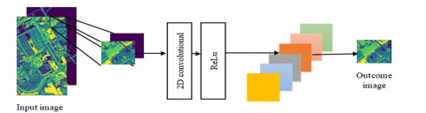
Our 2D-CNN method is separated into three sections, as exposed in Figure 1: patch extraction, feature extraction, and label identification. We initially extract a tiny patch focused on every pixel from a hyperspectral image to serve as the essential feature. The feature maps of these patches are then developed with a built-in deep learning method. As a concluding phase, the feature map of the similar patch is utilized to categorize every picture element label. We don't include the pooling layers for any of the four methods to retain as much pixel information as possible. The following diagram depicts the 2D-CNN methods of three-phase processing.
Figure 1. 2D convolutional process of 2D-CNN method
Assuming that a hyperspectral image of size W×H×C is provided to us, where H and W stand for the image's height and width, respectively, and C stands for the number of spectral bands, Predicting the labels for every pixel in the image is our goal. Given that labels for spatially nearby pixels frequently match, the proposed approach should consider "spatial coherence." The initial step in the presented method of processing is to extract a P×P×C patch for every picture element. A pixel, the patch's center, is the location about which every patch is built. There might not be enough data for the picture elements close to the edge of the image to create a patch that is the expected size. As a result, we use the mirror-padding process of picture elements to generate the spatial context.
The next processing stage handles every extracted patch as a separate image with multiple channels. To extract the feature maps for the patch, we can thus use a deep CNN method with 2D layers. The 2D-CNN operator at every layer is more appropriately stated in the subsequent Eq. (1):
$u_{i j}^{x y}=G\left(d_{i j}+\sum_s \sum_{a=0}^{H_i-1} \sum_{b=0}^{W_j-1} \vartheta_{i j}^{s a b} u_{i-1}^{(x+a)(y+b)}\right)$ (1)
Here, uⅈjxy stands for the outcome at point (x, y) of the j is amount of feature map at the i layer, dij denotes the bias term, G(.) represents the activation function of the layer, and s indexes over the set of feature maps of the (ⅈ-1)th layer, which are the inputs to the ith layer. Where i denotes the specific layer under consideration. Hi and Wj are the width and height of this kernel, and ϑijsab is the point (a,b) of the convolution kernel that connects the ith feature map to the jth feature map. Use the ReLU function as the initiation G function for the proposed approach, which is described in Eq. (2) below:
$G(x)=\max (0, x)$ (2)
Three convolutional layers are used in our 2D-CNN model. We ignore the pooling layers from the 2D-CNN method to protect the essential data of every picture element. The prediction is then built using a fully connected layer that inputs the feature maps from the previous 2D-CNN. In this case, we use the soft-max function to calculate the probability for every class. For multiple categorizations, the soft-max function extends the sigmoid function. The cross-entropy process was also chosen as the actual function that will guide the Backpropagation created training operation.
Here, M and c stand in for every variable in our 2D-CNN method. We use the following soft-max function to convert the scores gd (Ii,j,l; (M,c)) of every class of interest dϵ{1,…,N} into the qualified possibilities as we train the 2D-CNN method by maximizing the likelihood (3):
$q\left(\left.d\right|_{i, j, l} ;(M, c)\right)=\frac{e^{g_d\left(I_{i, j, l} ;(M, c)\right)}}{\sum_{r \in\{1, \ldots, N\}} e^{g_r\left(I_{i, j, l} ;(M, c)\right)}}$ (3)
By reducing the negative log-likelihood used in the training
process, the parameters (M,c) are learned (4).
$L(M, c)=-\sum_{I_{i, j, l}} \ln q\left(I_{i, j, l} \mid I_{i, j, l} ;(M, c)\right)$ (4)
When the pixel at the position (i,j) in the image Il has the proper class label, denoted by the notation Ii,j,l. Adam optimizer with Backpropagation, maximizes the objective function. Using the argmax process, the outcome layer of the presented approach forecasts the label of the picture element at (i,j) of a data point I at testing time (5).
$\widehat{l_{l, j}}=\arg \max q\left(\left.d\right|_{i, j, l} ;(M, c)\right) \cdot d \epsilon\{1, \ldots, N\}$ (5)
3.2 The 3D-CNN method (3D-CNN)
The previous is taken by examining the identical area with various spectral bands. Whereas the final is not, this is one of the key distinctions between a HSI and a common image. It is preferable to consider hyperspectral correlations since the data created by hyperspectral bands has some connections; for example, nearby hyperspectral bands provide the same images. The spatial context can be utilized by the 2D-CNN method, but the hyperspectral correlations are discarded. To create a 3D-CNN process to deal with this problem.
The process specifics of the 3D-CNN method are comparable to the 2D-CNN approach, as illustrated in Figure 2. The primary distinction is that the 3D-CNN process has an additional reordering phase. The C hyperspectral bands are reordered in this phase in an increasing direction. This sequential ordering of images of associated spectral bands can maintain their correlations in a spectral context. The two methods' patch extraction and label recognition phases are remarkably comparable. Rather than using a 2D convolution operator for the feature extraction stage, the 3D-CNN method is utilized. The 3D convolution operation is explicitly written in the following Eq. (6):
$\begin{aligned} & u_{i j}^{x y}=G\left(d_{i j}+\sum_s \sum_{a=0}^{H_i-1} \sum_{b=0}^{W_i-1} \sum_{k=0}^{C_i-1} \vartheta_{i j s}^{k a b} u_{(i-1) s}^{(x+a)(y+b)(z+k)}\right)\end{aligned}$ (6)
Here, ϑijskab is the point at the (a,b,k)th location of the kernel associated with the sth feature map of the prior layer, where Ci is the size of the 3D kernel together with the spectral dimension and j is the number of kernels in the ⅈth layer. Once more, activation function G is assumed to be the ReLU function.
Figure 2. 3D convolutional process of 3D-CNN method
Figure 2 depicts the 3D convolution technique. We can see that a 3D patch is subject to the 3-D convolution process in stages, such as inner to outer, top to bottom, and left to right. A convolution layer is created at every stage and positioned in the appropriate location on the feature map. As a result of this technique, a feature map is a smaller 3D cube. Similar to training a 2D-CNN method, training a 3D-CNN method involves computing the possibility of every class using the soft-max function. Moreover, by expanding the log-likelihood of the training set, we express the analysis procedure as an optimization issue. Adam optimizer with Backpropagation is additionally used for network training.
3.3 The recurrent 2D-CNN method (R-2D-CNN)
As the categorization of a picture element depends on the properties of a tiny patch adjacent to the picture element rather than the features instantly committed to the picture element, the 2D-CNN method, as previously mentioned, may generate undesirable noise even if it can take advantage of the spatial context. To create an R-2D-CNN method to utilize the spatial environment more effectively. A multiscale deep neural network is used by the R-2D-CNN method to fuse numerous shrinking patches into multiple instances, which it then uses to make predictions.
To make things clear, we refer to the instances as the first phase, the second phase, and the qth phase, correlating after the larger patches to the minor patches, here the Pth phase frequently correlates to the picture element for categorization, i.e., a 1×1 patch. A R-CNN structure, in which a fundamental 2D-CNN block is repeatedly reused, makes up the R-2D-CNN deep neural network. It extracts the feature maps for the initial-phase instances using the essential 2D-CNN block. The similar 2D-CNN block extracts the following-phase feature maps by concatenating these feature maps with the second-phase representatives. Up until the qth level instances are fused, this process is repeated. The probability of every class is calculated after applying a soft-max layer. We can examine the spatial context data and concentrate additional on the data closest to the picture element for categorization by using the numerous shrunk patches. As a result, the undesirable noises might decrease.
Figure 3. R-2D-CNN method contains two fundamental 2D-CNN
Figure 3 represents the foremost framework of the R-2D-CNN method. At the qth phase, the system is sustained with the original "feature image" Gq of F +C, which consists of H feature maps for the (q-1)th instances, C is HSI for the qth occurrences, and 1≤ q≤ Q. F means the number of feature maps created by the 2D-CNN method. The method is described in formal terms as follows (7):
$G^q=\left[G\left(G^{q-1}, I_{i, j, l}^q\right)\right], G^1=\left[0, I_{i, j, l}\right]$ (7)
where, Ii,j,l refers to the actual patch that encloses the picture element at coordinates (i,j) on the training image l. Since there is no occurrence since a prior to build the feature maps, the network just accepts the actual image as input in the first phase. Despite having multiple phases, the R-2D-CNN method problem does not improve with the number of phases. The explanation is that the parameters for many levels are expected, as shown in Figure 3.
The gradients are generated utilizing the Backpropagation through time (BPTT) procedure throughout the Backpropagation method, just like the 2D-CNN model during model training. More specifically, we train the method using the BPTT algorithm after first unfolding the network, as depicted in Figure 3. Contrary to the 2D-CNN method, the recurrent multilevel architecture forces us to acquire the network limitations (W, b) through a novel loss function (8). The loss function is established using (7):
$I(G)+I(G \circ G)+\cdots+I\left(G \circ{ }^q G\right)$ (8)
I(G) is the log-likelihood of the 2D-CNN model established in (3), ◦q stands for the composition operation carried out q times. In order to provide the appropriate label at the location, each network instance is trained (i,j). The R-2D-CNN method can learn from its errors and fix them in subsequent iterations. The R-2D-CNN model can also categorize dependences, which involves predicting an instance's label based on the label of an earlier occurrence centered on location (i,j).
It is important to note that the sizes of the tiered sample in order for the R-2D-CNN method to be appropriately planned for the instances to be combined by the feature maps of the prior instances. To achieve this, we must initially determine how a feature map's size variations at what time is employed in a 2D convolution layer. Here rzs-1 represents the (s-1)th convolution layer's feature map size. Then, the formula (9) below is utilized to calculate the size of the feature map generated by the mth convolution layer:
$r Z_s=\frac{r Z_{s-1}-c V_s}{t V_s}+11$ (9)
where, tVs is the stride size, and cVs is the size of the sth layer's convolution kernel. To determine the size of a feature map created by the 2D-CNN block (8). As a result, we can calculate the instances' proper sizes for various categories.
3.4 The recurrent 3D-CNN method (R-3D-CNN)
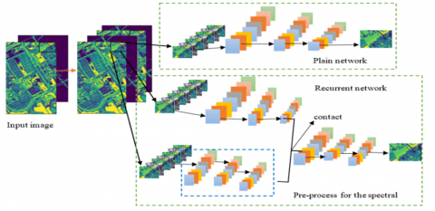
We created the R-3D-CNN method to use hyperspectral images' spatial and spectral contexts more effectively. Like the R-2D-CNN model, multilevel RNNs that gradually shrink a patch into multiple instances also support the R-3D-CNN paradigm. R-2D-CNN method and the R-3D-CNN method differ primarily in two ways. The primary distinction is that the prior uses the 3D convolution process, while the last utilizes their 2D equivalents. As a result, the R-3D-CNN method could be a recurrent addition to the 3D-CNN process. The second distinction is that feature maps produced at the current level must be concatenated with instances from the following level once they have been pre-processed. We use 3D convolution layers for this purpose, which causes the spectral bands to have variable lengths. In order to adjust to the shifting sizes, we must pre-process the instances of the following level using specific 3D spectral channel convolution techniques.
An illustration of the proposed R-3D-CNN method is shown in Figure 4. A multi-layer RNN with P-tiered instances makes up the model. With the R-2D-CNN method, the matching feature maps are extracted using a "simple" 3D convolution network and then concatenated with the instance from the following phase to develop novel feature maps at every phase. This approach is repetitive until completely tiered samples have been included. A pre-processing step is added to the spectral networks to maintain consistency between the sizes of feature maps at the present phase and the sizes of the occurrences at the following phase. The cross-entropy objective function is next applied, and a soft-max layer is lastly added.
The BPTT method is once again used in the optimization process. The R-3D-CNN approach's complexity is comparable to the R-2D-CNN approach since the recurrent structure uses the same network parameters at several stages. We must reorder the hyperspectral images in the 3D-CNN method by spectral band ordering. As with the R-2D-CNN paradigm, the size of tiered instances must also be wisely calculated.
To assess the proposed approaches' effectiveness, we selected two publicly accessible hyperspectral image data sets. We also used LORSAL, MFL, and SVM-3-DG as the baselines for performance comparison. We employed two performance metrics: the average accuracy of every class, the overall accuracy of every class indicated on AA and OA, the kappa coefficient (Kc), and time consumption.
4.1 Datasets
Pavia University scene: Using the ROSIS [Reflective Optics System Imaging Spectrometer] sensor, this hyperspectral image data set captures Pavia University in Italy. The image data collection has a spatial resolution of 610×340 pixels and 103 hyperspectral bands. It contains spatial information with fine details, enabling the observation of objects and features within the scene at a high level of detail. Spectrally, it covers a range of contiguous bands, providing detailed spectral information for each pixel. It covers various terrains, buildings, vegetation, and urban landscapes within the university premises. Nine classes are designated in the image, as seen in Figure 7(e): tree, asphalt, bitumen, gravel, metal sheet, shadow, bricks, meadow, and soil.
Indian pines scene: The AVIRIS sensor captures remote sensing images of Indian pines in north-western India. The data set was obtained in 1992. The dataset represents a snapshot of the area captured during the specific time of the AVIRIS flight in 1992. It encompasses various land cover types, such as agricultural fields, forests, and other natural and man-made features. The hyperspectral image has a spatial resolution of 145×145, a picture element, and 224 hyperspectral bands. Only 200 hyperspectral bands were selected because there were noisy bands present. The bands 104-108, 150-163, and 220 that covered the water-absorbing zones are eliminated. There are 16 classes in the actual data that are not all exclusive. For our experiment, we separated the labeled data into 70 percent of training sets and 30 percent of testing sets at random, as shown in Figure 7(a). In order to balance computational efficiency and model convergence, batch sizes ranging from 17 to 62 are used in experiments on these datasets. The learning rate parameters of these two datasets are tuned between 0.001 and 0.01. Adam Optimizer is used due to its adaptive learning rates and efficiency in optimizing CNNs. For effective regularization, dropout rates of 0.32 are employed in fully connected layers to prevent overfitting.
4.1.1 Outcomes for the Pavia University scene
The deep learning models used in this experiment have structures similar to those used in the original Indian pines scene experiment. The main modification is several parameters to correlate to the 102 hyperspectral bands of the improved database. Recall that the first data set had 200 bands. Created on the Pavia University scene database, Table 1 shows the experimental findings for each approach.
Figure 4. Network parameters for R-3D-CNN method across multiple shared levels
Table 1. Categorization outcomes of the Pavia University scene
|
Classes |
LORSAL [43] |
MFL [46] |
SVM-3DG [47] |
2D-CNN Method |
3D-CNN Method |
R-2D-CNN Method |
R-3D-CNN Method |
|
1 |
91.2 |
100 |
99.45 |
93.21 |
99.41 |
99.76 |
100 |
|
2 |
96.92 |
99.93 |
99.86 |
99.87 |
100 |
100 |
100 |
|
3 |
64.07 |
93.64 |
87.12 |
93.34 |
98.15 |
99.34 |
100 |
|
4 |
88.57 |
98.59 |
99.67 |
88.04 |
95.88 |
94.65 |
100 |
|
5 |
99.75 |
99.5 |
100 |
92.67 |
98.97 |
99.03 |
100 |
|
6 |
57.76 |
99.67 |
99.07 |
99.36 |
99.96 |
100 |
100 |
|
7 |
59.05 |
99.75 |
95.73 |
92.67 |
99.01 |
99.02 |
100 |
|
8 |
80.45 |
99.1 |
96.38 |
94.19 |
99.35 |
100 |
100 |
|
9 |
97.89 |
100 |
98.94 |
88.56 |
83.56 |
96.06 |
99.97 |
|
OA |
86.74 |
99.42 |
98.62 |
96.35 |
98.89 |
99.63 |
99.98 |
|
AA |
81.74 |
98.91 |
97.36 |
98.55 |
97.14 |
98.65 |
99.99 |
|
Kc |
- |
- |
- |
93.31 |
95.02 |
97.24 |
99.1 |
|
Time (s) |
- |
- |
- |
125.4 |
156.78 |
238.14 |
293.74 |
Once more, it is clear that the presented R-3D-CNN exceeds the R-2D-CNN methods, the LORSAL method, the MFL method, and the SVM-3DG method. Compared to the MFL, which had an OA of 99.42 percent, the R-3D-CNN model's OA is 99.988 percent, a difference of 0.56%. And when we consider lowering error rates, the R-3D-CNN method surpasses the MFL technique by more than 95%. Results from the 3D-CNN and 2D-CNN models are equivalent to those from the SVM-3-DG approach. The LORSAL classifier performs the least well of all the techniques. The categorization outcomes for all the processes are illustrated in Figure 5.
Figure 5. Pavia University scene (a) Ground truth image, (b) 2D-CNN result, (c) 3D-CNN result (d) R-2D-CNN result and (e) R-3D-CNN result
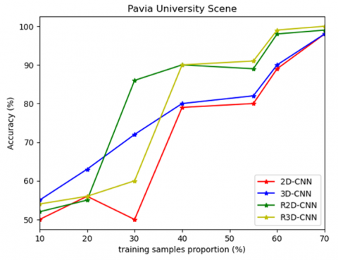
Figure 6. Effect of training sample proportion vs. Accuracy for Pavia University scene
In this experiment, we examined how different training sample sizes affected the evaluation of the presented deep learning techniques. Evaluate the training sample proportion and accuracy for the Pavia University scene database. The presented deep learning methods, 3D-CNN, R-3D-CNN, 2D-CNN, and R-2D-CNN, demonstrate improved performance as training sets increase, as shown in Figure 6.
4.1.2 Outcomes for the Indian pines scene
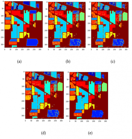
The investigational findings using different data sets are then reported. The results of every method are displayed in Table 2. We note that the R-3D-CNN method, whose OA is 99.97%, performs best. Even if the MFL's OA is 97.05%, the R-3D-CNN method performs better than it by 0.32% when error rates are considered.
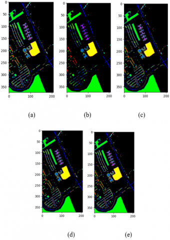
The primary justification for this is that the R-3D-CNN method includes spectral and spatial contexts. The previous is incidental using the 3-D convolution procedure, and the last uses the recurrent multilevel structure. The R-2D-CNN method is evaluated as the next greatest in AA and OA, and the LORSAL, the 3D-CNN method, and the 2D-CNN method follow it. Despite not considering spectral correlations, the R-2D-CNN's structures may efficiently record the spatial context for consequent data categorization. Our investigational outcomes show the spatial context is more essential than the spectral correlations for HSI categorization. The findings of MFL are superior to those of SVM-3-DG and LORSAL, as shown in Table 2. Yet, its performance is significantly inferior compared to different deep learning algorithms. Because it can extract EMAP data relevant to the spectral-spatial contexts, the MFL obtains a comparable evaluation to that of the 3D-CNN and the 2D-CNN approaches as a potential classification approach. A visual comparison of the effectiveness of each technique is displayed in Figure 7.
Table 2. Categorization outcomes of Indian pines scene
|
Classes |
LORSAL [43] |
MFL [46] |
SVM-3DG [47] |
2D-CNN Method |
3D-CNN Method |
R-2D-CNN Method |
R-3D-CNN Method |
|
1 |
85.71 |
85.71 |
64.29 |
74.23 |
87.76 |
79.94 |
100 |
|
2 |
89.88 |
96.24 |
80 |
96.76 |
97.23 |
99.86 |
100 |
|
3 |
82.04 |
92.65 |
73.47 |
97.82 |
98.49 |
99.11 |
100 |
|
4 |
82.61 |
97.1 |
97.1 |
75.67 |
99.76 |
100 |
100 |
|
5 |
91.61 |
97.2 |
91.61 |
98.46 |
98.59 |
98.31 |
100 |
|
6 |
99.08 |
99.54 |
97.7 |
97.29 |
98.14 |
100 |
100 |
|
7 |
100 |
100 |
62.5 |
100 |
100 |
88.65 |
100 |
|
8 |
100 |
100 |
100 |
100 |
100 |
100 |
100 |
|
9 |
83.33 |
100 |
100 |
100 |
100 |
100 |
100 |
|
10 |
85.81 |
92.04 |
75.78 |
98.85 |
99.21 |
99.32 |
100 |
|
11 |
88.83 |
98.5 |
95.37 |
99.98 |
99.92 |
100 |
99.92 |
|
12 |
88.64 |
96.02 |
86.36 |
97.31 |
98.56 |
99.87 |
99.03 |
|
13 |
100 |
98.36 |
98.36 |
100 |
97.65 |
99.43 |
100 |
|
14 |
96.02 |
99.47 |
97.08 |
99.42 |
100 |
100 |
100 |
|
15 |
83.33 |
97.37 |
100 |
95.23 |
94.14 |
99.45 |
97.43 |
|
16 |
85.71 |
100 |
78.21 |
100 |
100 |
97.59 |
97.32 |
|
OA |
90.1 |
97.05 |
89.44 |
98.13 |
98.25 |
99.35 |
99.97 |
|
AA |
88.47 |
96.89 |
87.61 |
97.68 |
99.09 |
97.59 |
99.6 |
|
Kc |
- |
- |
- |
97.07 |
97.25 |
97.38 |
99.2 |
|
Time(s) |
- |
- |
- |
149.47 |
179.8 |
271.26 |
322.18 |
Table 3. Descriptive statistics of Pavia scene
|
Statistics |
LORSAL [43] |
MFL [46] |
SVM-3DG [47] |
2D-CNN Method |
3D-CNN Method |
R-2D-CNN Method |
R-3D-CNN Method |
|
Mean |
81.74 |
98.90889 |
97.35778 |
93.54556 |
97.14333 |
98.65111 |
99.99667 |
|
Standard Error |
5.719757 |
0.676585 |
1.378501 |
1.349262 |
1.748169 |
0.647271 |
0.003333 |
|
Median |
88.57 |
99.67 |
99.07 |
93.21 |
99.01 |
99.34 |
100 |
|
Mode |
99 |
100 |
99 |
92.67 |
99 |
100 |
100 |
|
Standard Deviation |
17.15927 |
2.029756 |
4.135504 |
4.047787 |
5.244507 |
1.941813 |
0.01 |
|
Sample Variance |
294.4406 |
4.119911 |
17.10239 |
16.38458 |
27.50485 |
3.770636 |
0.0001 |
|
Kurtosis |
-1.69887 |
7.66773 |
5.634035 |
-0.30016 |
7.555099 |
1.326689 |
9 |
|
Skewness |
-0.51764 |
-2.71734 |
-2.3034 |
0.381959 |
-2.70354 |
-1.5868 |
-3 |
|
Range |
41.99 |
6.36 |
12.88 |
11.83 |
16.44 |
5.35 |
0.03 |
|
Minimum |
57.76 |
93.64 |
87.12 |
88.04 |
83.56 |
94.65 |
99.97 |
|
Maximum |
99.75 |
100 |
100 |
99.87 |
100 |
100 |
100 |
|
Sum |
735.66 |
890.18 |
876.22 |
841.91 |
874.29 |
887.86 |
899.97 |
|
Count |
9 |
9 |
9 |
9 |
9 |
9 |
9 |
Table 4. Descriptive statistics of Indian pines scene
|
Statistics |
LORSAL [43] |
MFL [46] |
SVM-3DG [47] |
2D-CNN Method |
3D-CNN Method |
R-2D-CNN Method |
R-3D-CNN Method |
|
Mean |
90.1625 |
96.8875 |
87.36438 |
95.68875 |
98.09063 |
97.59563 |
99.60625 |
|
Standard Error |
1.689927 |
0.968596 |
3.28821 |
2.056763 |
0.789279 |
1.36826 |
0.225961 |
|
Median |
88.735 |
97.865 |
93.49 |
98.655 |
98.9 |
99.655 |
100 |
|
Mode |
100 |
100 |
100 |
100 |
100 |
100 |
100 |
|
Standard Deviation |
6.75971 |
3.874383 |
13.15284 |
8.227052 |
3.157116 |
5.473039 |
0.903843 |
|
Sample Variance |
45.69367 |
15.01085 |
172.9972 |
67.68439 |
9.96738 |
29.95416 |
0.816932 |
|
Kurtosis |
-1.38387 |
3.792907 |
-0.85985 |
4.448971 |
8.04569 |
7.82471 |
3.779605 |
|
Skewness |
0.468609 |
-1.8647 |
-0.74157 |
-2.3671 |
-2.70595 |
-2.83086 |
-2.23758 |
|
Range |
17.96 |
14.29 |
37.5 |
25.77 |
12.24 |
20.06 |
2.68 |
|
Minimum |
82.04 |
85.71 |
62.5 |
74.23 |
87.76 |
79.94 |
97.32 |
|
Maximum |
100 |
100 |
100 |
100 |
100 |
100 |
100 |
|
Sum |
1442.6 |
1550.2 |
1397.83 |
1531.02 |
1569.45 |
1561.53 |
1593.7 |
|
Count |
16 |
16 |
16 |
16 |
16 |
16 |
16 |
Figure 7. Indian pines scene (a) Ground truth image, (b) 2D-CNN result, (c) 3D-CNN result (d) R-2D-CNN result and (e) R-3D-CNN result
Table 3 summarizes the comparison of descriptive statistics method to describe the features of the Pavia University dataset.
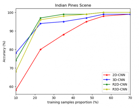
Figure 8. Effect of training sample proportion vs. Accuracy for Indian pines scene.
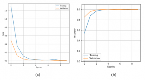
Figure 9. (a) R-3D-CNN Loss vs epochs and (b) R-3D-CNN Accuracy vs epochs
Figure 8 shows the performance of the training sample proportion vs. accuracy for the Indian pines scene dataset, showing improved performance as training data increases.
Table 4 summarizes the comparison of descriptive statistics methods to describe the features of the Indian Pine dataset.
The graphs of accuracy and loss over training and validation processes on diverse subjects are depicted in Figure 9.
In this study, we investigated deep learning approaches for categorizing HSI. Four deep learning models have been created and developed, including the 3D-CNN, R-3D-CNN, 2D-CNN, and 2D-CNN. Based on two freely accessible HSI data sets, rigorous experiments were carried out. Our experimental findings support the excellence of these deep learning approaches over more conventional machine learning techniques like LORSAL, MFL, and SVM-3DG. Due to its 3D convolutional fixer and recurrent network architecture, it can efficiently utilize spatial and spectral contexts. The presented R-3D-CNN method frequently overcomes competing approaches for the maximum of the database and connects more quickly. If categorization evaluation is defined regarding error rate, the R-3D-CNN and R-2D-CNN perform more than 30% better than the baselines. The categorization outcomes of the Indian pines scene using R-3D-CNN provide efficient performance based on kappa coefficient, time consumption, overall accuracy, and average accuracy of 99.6%, 322.18 seconds, 99.97%, and 97.6%, respectively. Similarly, the categorization outcomes of the Pavia University Scene using R-3D-CNN are efficient performance-based kappa coefficient, time consumption, overall accuracy, and average accuracy of 99.1%, 293.74 seconds, 99.98%, and 99.99%, respectively. Although the proposed approaches are superior, deep learning methods frequently require more training data than conventional machine learning techniques. Processing of Pavia data cubes and Indian Pine data cubes with numerous spectral bands leads to increased training and inference times. Consequently, adding previous field data to the provided deep learning methods resolves a significant future analysis area.
[1] Van der Meer, F.D., Van der Werff, H.M., Van Ruitenbeek, F.J., Hecker, C.A., Bakker, W.H., Noomen, M.F., Woldai, T. (2012). Multi-and hyperspectral geologic remote sensing: A review. International Journal of Applied Earth Observation and Geoinformation, 14(1): 112-128. https://doi.org/10.1016/j.jag.2011.08.002
[2] Zhang, C., Kovacs, J.M. (2012). The application of small unmanned aerial systems for precision agriculture: A review. Precision Agriculture, 13: 693-712. https://doi.org/10.1007/s11119-012-9274-5
[3] Pan, B., Shi, Z., An, Z., Jiang, Z., Ma, Y. (2016). A novel spectral-unmixing-based green algae area estimation method for GOCI data. IEEE Journal of Selected Topics in Applied Earth Observations and Remote Sensing, 10(2): 437-449. https://doi.org/10.1109/JSTARS.2016.2585161
[4] Hughes, G. (1968). On the mean accuracy of statistical pattern recognizers. IEEE Transactions on Information Theory, 14(1): 55-63. https://doi.org/10.1109/TIT.1968.1054102
[5] Zhang, X., Liang, Y., Zheng, Y., An, J., Jiao, L.C. (2016). Hierarchical discriminative feature learning for hyperspectral image classification. IEEE Geoscience and Remote Sensing Letters, 13(4): 594-598. https://doi.org/10.1109/LGRS.2016.2528883
[6] Prasad, S., Bruce, L.M. (2008). Limitations of principal components analysis for hyperspectral target recognition. IEEE Geoscience and Remote Sensing Letters, 5(4): 625-629. https://doi.org/10.1109/LGRS.2008.2001282
[7] Bachmann, C.M., Ainsworth, T.L., Fusina, R.A. (2006). Improved manifold coordinate representations of large-scale hyperspectral scenes. IEEE Transactions on Geoscience and Remote Sensing, 44(10): 2786-2803. https://doi.org/10.1109/TGRS.2006.881801
[8] Du, B., Zhang, L., Zhang, L., Chen, T., Wu, K. (2012). A discriminative manifold learning based dimension reduction method for hyperspectral classification. International Journal of Fuzzy Systems, 14(2): 272-277.
[9] Sun, W., Zhang, L., Du, B., Li, W., Lai, Y.M. (2015). Band selection using improved sparse subspace clustering for hyperspectral imagery classification. IEEE Journal of Selected Topics in Applied Earth Observations and Remote Sensing, 8(6): 2784-2797. https://doi.org/10.1109/JSTARS.2015.2417156
[10] Persello, C., Bruzzone, L. (2015). Kernel-based domain-invariant feature selection in hyperspectral images for transfer learning. IEEE Transactions on Geoscience and Remote Sensing, 54(5): 2615-2626. https://doi.org/10.1109/TGRS.2015.2503885
[11] Liao, W., Bellens, R., Pižurica, A., Philips, W., Pi, Y. (2012). Classification of hyperspectral data over urban areas based on extended morphological profile with partial reconstruction. In Advanced Concepts for Intelligent Vision Systems: 14th International Conference, Brno, Czech Republic, pp. 278-289. https://doi.org/10.1007/978-3-642-33140-4_25
[12] Ghamisi, P., Dalla Mura, M., Benediktsson, J.A. (2014). A survey on spectral-spatial classification techniques based on attribute profiles. IEEE Transactions on Geoscience and Remote Sensing, 53(5): 2335-2353. https://doi.org/10.1109/TGRS.2014.2358934
[13] Li, J., Khodadadzadeh, M., Plaza, A., Jia, X., Bioucas-Dias, J.M. (2015). A discontinuity preserving relaxation scheme for spectral-spatial hyperspectral image classification. IEEE Journal of Selected Topics in Applied Earth Observations and Remote Sensing, 9(2): 625-639. https://doi.org/10.1109/JSTARS.2015.2470129
[14] Khodadadzadeh, M., Li, J., Plaza, A., Ghassemian, H., Bioucas-Dias, J.M., Li, X. (2014). Spectral-spatial classification of hyperspectral data using local and global probabilities for mixed pixel characterization. IEEE Transactions on Geoscience and Remote Sensing, 52(10): 6298-6314. https://doi.org/10.1109/TGRS.2013.2296031
[15] Fauvel, M., Tarabalka, Y., Benediktsson, J.A., Chanussot, J., Tilton, J.C. (2012). Advances in spectral-spatial classification of hyperspectral images. Proceedings of the IEEE, 101(3): 652-675. https://doi.org/10.1109/JPROC.2012.2197589
[16] Hinton, G.E., Salakhutdinov, R.R. (2006). Reducing the dimensionality of data with neural networks. Science, 313(5786): 504-507. https://doi.org/10.1126/science.1127647
[17] Krizhevsky, A., Sutskever, I., Hinton, G.E. (2017). Imagenet classification with deep convolutional neural networks. Communications of the ACM, 60(6): 84-90. https://doi.org/10.1145/3065386
[18] Sun, Y., Liang, D., Wang, X., Tang, X. (2015). Deepid3: Face recognition with very deep neural networks. arXiv preprint arXiv:1502.00873. https://doi.org/10.48550/arXiv.1502.00873
[19] Zhang, L., Zhang, L., Du, B. (2016). Deep learning for remote sensing data: A technical tutorial on the state of the art. IEEE Geoscience and Remote Sensing Magazine, 4(2): 22-40. https://doi.org/10.1109/MGRS.2016.2540798
[20] Chen, Y., Lin, Z., Zhao, X., Wang, G., Gu, Y. (2014). Deep learning-based classification of hyperspectral data. IEEE Journal of Selected Topics in Applied Earth Observations and Remote Sensing, 7(6): 2094-2107. https://doi.org/10.1109/JSTARS.2014.2329330
[21] Ma, X., Geng, J., Wang, H. (2015). Hyperspectral image classification via contextual deep learning. EURASIP Journal on Image and Video Processing, 2015: 1-12. https://doi.org/10.1186/s13640-015-0071-8
[22] Liu, Y., Cao, G., Sun, Q., Siegel, M. (2015). Hyperspectral classification via deep networks and superpixel segmentation. International Journal of Remote Sensing, 36(13): 3459-3482. https://doi.org/10.1080/01431161.2015.1055607
[23] Tao, C., Pan, H., Li, Y., Zou, Z. (2015). Unsupervised spectral–spatial feature learning with stacked sparse autoencoder for hyperspectral imagery classification. IEEE Geoscience and Remote Sensing Letters, 12(12): 2438-2442. https://doi.org/10.1109/LGRS.2015.2482520
[24] Zhao, W., Guo, Z., Yue, J., Zhang, X., Luo, L. (2015). On combining multiscale deep learning features for the classification of hyperspectral remote sensing imagery. International Journal of Remote Sensing, 36(13): 3368-3379. https://doi.org/10.1080/2150704X.2015.1062157
[25] Makantasis, K., Karantzalos, K., Doulamis, A., Doulamis, N. (2015). Deep supervised learning for hyperspectral data classification through convolutional neural networks. In 2015 IEEE International Geoscience and Remote Sensing Symposium (IGARSS): Milan, Italy, pp. 4959-4962. https://doi.org/10.1109/IGARSS.2015.7326945
[26] Hu, W., Huang, Y., Wei, L., Zhang, F., Li, H. (2015). Deep convolutional neural networks for hyperspectral image classification. Journal of Sensors, 2015: 1-12. https://doi.org/10.1155/2015/258619
[27] Liang, H., Li, Q. (2016). Hyperspectral imagery classification using sparse representations of convolutional neural network features. Remote Sensing, 8(2): 99. https://doi.org/10.3390/rs8020099
[28] Romero, A., Gatta, C., Camps-Valls, G. (2015). Unsupervised deep feature extraction for remote sensing image classification. IEEE Transactions on Geoscience and Remote Sensing, 54(3): 1349-1362. https://doi.org/10.1109/TGRS.2015.2478379
[29] Chen, Y., Jiang, H., Li, C., Jia, X., Ghamisi, P. (2016). Deep feature extraction and classification of hyperspectral images based on convolutional neural networks. IEEE Transactions on Geoscience and Remote Sensing, 54(10): 6232-6251. https://doi.org/10.1109/TGRS.2016.2584107
[30] Chan, T.H., Jia, K., Gao, S., Lu, J., Zeng, Z., Ma, Y. (2015). PCANet: A simple deep learning baseline for image classification. IEEE Transactions on Image Processing, 24(12): 5017-5032. https://doi.org/10.1109/TIP.2015.2475625
[31] Pan, B., Shi, Z., Zhang, N., Xie, S. (2016). Hyperspectral image classification based on nonlinear spectral–spatial network. IEEE Geoscience and Remote Sensing Letters, 13(12): 1782-1786. https://doi.org/10.1109/LGRS.2016.2608963
[32] Deng, J., Dong, W., Socher, R., Li, L. J., Li, K., Fei-Fei, L. (2009). Imagenet: A large-scale hierarchical image database. In 2009 IEEE Conference on Computer Vision and Pattern Recognition, Miami, FL, USA, pp. 248-255. https://doi.org/10.1109/CVPR.2009.5206848
[33] Zhao, W., Du, S. (2016). Spectral–spatial feature extraction for hyperspectral image classification: A dimension reduction and deep learning approach. IEEE Transactions on Geoscience and Remote Sensing, 54(8): 4544-4554. https://doi.org/10.1109/TGRS.2016.2543748
[34] Pan, B., Shi, Z., Xu, X. (2018). MugNet: Deep learning for hyperspectral image classification using limited samples. ISPRS Journal of Photogrammetry and Remote Sensing, 145: 108-119. https://doi.org/10.1016/j.isprsjprs.2017.11.003
[35] Zhong, Z., Li, J., Luo, Z., Chapman, M. (2017). Spectral–spatial residual network for hyperspectral image classification: A 3-D deep learning framework. IEEE Transactions on Geoscience and Remote Sensing, 56(2): 847-858. https://doi.org/10.1109/TGRS.2017.2755542
[36] Yang, X., Ye, Y., Li, X., Lau, R. Y., Zhang, X., Huang, X. (2018). Hyperspectral image classification with deep learning models. IEEE Transactions on Geoscience and Remote Sensing, 56(9): 5408-5423. https://doi.org/10.1109/TGRS.2018.2815613
[37] Ma, X., Geng, J., Wang, H. (2015). Hyperspectral image classification via contextual deep learning. EURASIP Journal on Image and Video Processing, 2015: 1-12. https://doi.org/10.1186/s13640-015-0071-8
[38] Pan, B., Shi, Z., Xu, X. (2017). R-VCANet: A new deep-learning-based hyperspectral image classification method. IEEE Journal of Selected Topics in Applied Earth Observations and Remote Sensing, 10(5): 1975-1986. https://doi.org/10.1109/JSTARS.2017.2655516
[39] Liu, P., Zhang, H., Eom, K.B. (2016). Active deep learning for classification of hyperspectral images. IEEE Journal of Selected Topics in Applied Earth Observations and Remote Sensing, 10(2): 712-724. https://doi.org/10.1109/JSTARS.2016.2598859
[40] Hu, W., Huang, Y., Wei, L., Zhang, F., Li, H. (2015). Deep convolutional neural networks for hyperspectral image classification. Journal of Sensors, 2015, 1-12. https://doi.org/10.1155/2015/258619
[41] Sellami, A., Tabbone, S. (2022). Deep neural networks-based relevant latent representation learning for hyperspectral image classification. Pattern Recognition, 121: 108224. https://doi.org/10.1016/j.patcog.2021.108224
[42] Liu, B., Yu, A., Yu, X., Wang, R., Gao, K., Guo, W. (2020). Deep multiview learning for hyperspectral image classification. IEEE Transactions on Geoscience and Remote Sensing, 59(9): 7758-7772. https://doi.org/10.1109/TGRS.2020.3034133
[43] Chen, Y., Nasrabadi, N.M., Tran, T.D. (2012). Hyperspectral image classification via kernel sparse representation. IEEE Transactions on Geoscience and Remote Sensing, 51(1): 217-231. https://doi.org/10.1109/TGRS.2012.2201730
[44] Huang, Q., Jia, C.K., Zhang, X., Ye, Y. (2017). Learning discriminative subspace models for weakly supervised face detection. IEEE Transactions on Industrial Informatics, 13(6): 2956-2964. https://doi.org/10.1109/TII.2017.2753319
[45] Ma, X., Liu, Q., He, Z., Zhang, X., Chen, W.S. (2016). Visual tracking via exemplar regression model. Knowledge-Based Systems, 106: 26-37. https://doi.org/10.1016/j.knosys.2016.05.028
[46] Li, J., Huang, X., Gamba, P., Bioucas-Dias, J.M., Zhang, L., Benediktsson, J.A., Plaza, A. (2014). Multiple feature learning for hyperspectral image classification. IEEE Transactions on Geoscience and Remote sensing, 53(3): 1592-1606. https://doi.org/10.1109/TGRS.2014.2345739
[47] Cao, X., Xu, L., Meng, D., Zhao, Q., Xu, Z. (2017). Integration of 3-dimensional discrete wavelet transform and Markov random field for hyperspectral image classification. Neurocomputing, 226: 90-100. https://doi.org/10.1016/j.neucom.2016.11.034