Elif Akarsu*![]() | Tevhit Karacali
| Tevhit Karacali![]()
© 2024 The authors. This article is published by IIETA and is licensed under the CC BY 4.0 license (http://creativecommons.org/licenses/by/4.0/).
OPEN ACCESS
The article is about the classification of anomaly detection dataset-UCF videos obtained from Kaggle. The data set consists of 4-class video files. While three of them consist of different crimes and abnormal events such as Burglary, Explosion, and Fighting, one class consists of videos containing quotes from daily life that do not contain different crimes or events. 4-class videos from Anomaly-Detection-Dataset-UCF were used, Burglary consists of 100 videos, and videos from the other 3 classes are 50 each. and the number of frames of each video varies. First, each video in the dataset was converted into image frames. Because video data is the combination of multiple image frames to form a series. and each picture frame in this series contains important information. To obtain this information, feature information of each frame was extracted. This feature extraction process was carried out with 3 different algorithms. These algorithms; Alexnet is Vgg19 and Resnet18. However, during the feature acquisition phase, the last three layers from each of the 3 pre-training algorithms were removed with Transfer Learning, and 4 layers were manually added instead. and retrained Alexnet, vgg19, and resnet18 pretraining algorithms. Thus, it was aimed to obtain 1500 features instead of 1000 from each pre-training algorithm. It was aimed to obtain more detailed information about the videos by extracting more features. that is, it was aimed to increase the number of features with transfer learning. In other words, in this study, transfer learning was used for feature improvement and the effects of these three different algorithms on classification accuracy with the same parameters were investigated. The classification was done in MATLAB with an LSTM classifier as 5-fold. The data is divided into 5 parts with 5 folds, and different data are divided into test and train in each cycle. In this way, all data is reviewed and accuracy is verified at each fold. In the end, the classification result is obtained by averaging the accuracy in 5 cycles. Among the 3 algorithms, with both transfer learning and 5-fold classification, the lowest result was obtained from the Alexnet pre-training algorithm with 94.3% accuracy, Vgg19 with 96% accuracy, and the highest result was obtained from resnet18 with 98% accuracy. The content of the study focuses on examining these truths in detail.
artificial intelligence, deep learning, video classification, video dataset, pre-training algorithm
Video is a combination of multiple images. and it is created by combining these interconnected images into a series [1]. Usually, a video consists of 20-25 frames per second, the number of these frames directly affects the video quality [2]. A video can contain thousands of images, and multiple videos yield millions of images. The fact that the features of these millions of images can be obtained serially, one after another, without storing them anywhere and without taking up storage space, and distinguishing the obtained features reveals the importance of video classification. Based on all these, the picture frames that make up the videos are the primary data used in classification [1].
The size of the image data that makes up the videos is adjusted according to the size requested by the network. This can be done manually for a single image, but it is difficult and time-consuming to do it for a series of images without extracting the images into a folder. This poses a challenge in video classification.
The dimensions of the image inputs can be adjusted in a series to the desired size without requiring storage space. After the image dimensions are adjusted, the other steps of video classification are carried out [3]. When the studies are examined, it is seen that video classification with image data is based on 4 basic principles. It consists of extracting features from the training data from pre-training algorithms such as Alexnet, vgg19, and resnet18, selecting the video classifier, evaluating the appropriate classifier, and using the classifier to process the video [4].
A pretraining algorithm consists of multiple layers. CNN processes the image with various layers. Again; In a pre-training algorithm, convolutional layers in the network are the most important component of CNN algorithms. First of all, to extract the features of the image, a feature map is obtained by applying a multidimensional filter to the image in the convolution layer. Filters called multidimensional kernels are moved over the image step by step to extract features. As a result, a feature map is obtained. However, the dimensions of the feature map are smaller than the original image, and zeros are added to the structure in the fill layer to preserve the dimensions. A nonlinear function is obtained by passing the obtained features through the Relu layer. The purpose of this is to prevent the linear combination of outputs. Functions such as sigmoid and tanh were used in the past for nonlinear functions, but they had disadvantages in terms of the speed of the neural network.
For this reason, the ReLu function, which will work faster, has taken its place in the network. Thus, the amount of uncertain data is reduced by replacing the negative value in the Feature Map with "0". In other words, by eliminating ambiguous areas in the image and replacing them with zeros, obtaining information from image data becomes clearer and easier.
The next layer is the pooling layer. The task of the pooling layer is to reduce the size of the feature map [5] and the number of computations in the network. In this way, inconsistencies in the network are checked. and redundant data is reduced [6].
There are many pooling processes, but the most popular is maximum pooling. In other words, the filter takes the largest number in the area it covers. The flattening layer retrieves the data from the pool and transforms the data into a one-dimensional array. then the data passes to the fully connected layer. The fully connected layer of each of the 3 pre-training algorithms can give us 1000 features for each image. This study shows that with the help of transfer learning, we are not limited to 1000 features, but can obtain 1500 features from each image so that we can obtain more information about the images. Thus, we can gain a more advantageous situation when classifying videos by getting more information. The extracted features are taken from the fully connected layer [7]. and the classifier selection phase is started to classify the extracted features. There are many classification networks such as SVM and LSTM. However, in this study, the LSTM algorithm was preferred. It allows time-dependent classification as it has many adjustable hidden layers. Additionally, overfitting and underfitting are prevented with the dropout layer. Due to these features, using the LSTM classifier appears as an advantage.
In this study, the Anomaly-Detection-Dataset-UCF video dataset obtained from Kaggle was used. The dataset used is a 4-class video file consisting of Burglary, Explosion, Fighting, and normal videos [8]. Of these, burglary consists of 100 videos and the other 3 classes consist of 50 videos each. The picture frame numbers of each video are different from each other and each video frame consists of 320x240 size. Each video contains 30 frames per second. Additionally, all processed videos are in mp4 format. Our videos are processed by dividing them into picture frames. To obtain information from each framework, 3 different pre-training networks consisting of Alexnet, Resnet18, and Vgg19 were used. The reason for choosing these 3 different pre-training algorithms is that the image size accepted by Alexnet when entering the network is different from the other two. Another factor is that the number of layers and depth of each pre-training algorithm are different and it is desired to see what the consequences of these differences will be.
After the videos left the pre-training network, they were sent to the LSTM classifier and classified. Alexnet architecture has managed to preserve the "ImageNet" concept to a significant extent. Alexnet pre-training algorithm consists of 5 "convolutional layers" and 3 "fully connected layers". Then, the ReLu (Rectified Linear Unit) function was used as activation in the non-linear parts of Alexnet. The reason why ReLu has an advantage over Sigmoid is that it is more effective in training our model. is that it is fast. The other reason is that the sigmoid function causes the gradient problem to disappear.
If you notice, as the values of the sigmoid function grow or shrink, its derivative approaches zero. This problem is called "vanishing gradient". Therefore, it becomes difficult to update the weights in our model. If you consider a model too deeply, the first layers may have difficulty learning due to this problem. Alexnet is composed of 25 CNN layers and is the simplest pre-training network Alexnet, which includes 8 convolution layers. It is the simplest pre-training algorithm used today. however, it is an advantageous algorithm because it does not require high storage space and the classification results obtained are quite successful. The pre-trained network can separate input data into 1000 different categories. Alexnet can easily learn feature parameters for a range of multi-class images. Additionally, the input size of the image in the network is between 227 and 227 [9].
Vgg19 architecture presented by VGG Group (Oxford). High kernel sizes used in Alexnet architecture have been reduced. At Alexnet, the kernel sizes are not fixed after 5 and 3, starting with 11. VGG16, on the other hand, has fixed kernel sizes. The idea behind this is that 11×11 and 5×5 kernels can be repeated with more than one 3×3 kernel. Vgg19 has a total of 19 "convolutional" and "fully connected layers". There is also another version called Vgg19, which has 47 CNN layers and a more comprehensive structure. Vgg-19 is a 19-layer-deep nerve network. Generally, the pre-trained network can categorize images into 1000 object categories [10]. This number can be increased or decreased with the help of transfer learning. The input dimension of the picture on the network is between 224 and 224 [9].
Resnet18 contains a 71 CNN layer. As the number of CNN layers increases, the more complex the structure of the previous training network becomes. Images must be re-dimensioned independently of their size to enter the pre-training network. Resnet18 is an 18-layer deep convolutional neural network [9].
The fully connected layer of the pre-training network contains the count of classes, and the count of features of this network is 1000 [11]. that is, the network can classify a wide variety of data. It is preferred in studies due to both its depth and this feature. The input dimension of the picture on the network is between 224 and 224 Alexnet, Vgg19, Resnet18, and 1000 features were removed from the fully connected layer for each frame. 80% of the features removed are allocated for training and 20% for testing. this is done using a K-fold.
All data is multiplied by 5. test and training data are divided by each multiplier. During this division process, different data is trained on each floor. The videos were then classified with the LSTM classifier. When the video classification algorithm is examined, all videos delivered to the system are divided into frames. Videos converted to image frames are sent to the attribute extraction algorithm. Here, Vgg19 is introduced to pre-education networks such as Alexnet and Resnet18. Features of 4 different classes from the pre-training network are sent to the LSTM classifier and classified. The LSTM classifier was used because it has an adjustable number of layers, is a time-dependent function, contains a dropout detail that prevents overfitting, and this parameter is adjustable.
2.1 LSTM classifier
LSTM architecture consists of layers and memory cells with different functions. These memory cells are very advantageous in the long run. Because in Long-Short Term Memory Networks, it is possible to remember long-term information, that is, the oldest data. From this perspective, it is advantageous to use the LSTM classifier since historical information should not be forgotten within the scope of data processing. It also has LSTM memory bracketing mechanism. Thus, it can learn many features. Therefore, it is very advantageous in solving time-dependent problems [12]. Additionally, successful results have been achieved with LSTM architecture in speech [13], text processing [14], audio processing [15], image processing and most importantly classification [16] applications. LSTM cells contain gates that decide which information will be forgotten and which will be remembered. These gates are called entry gate, exit gate and forgetting gate, respectively [17].
The input gate controls (how much new value enters memory) and the output gate controls how much of the memory value is used to calculate the output activation of the memory cell. The forgetting gate decides what information will be stored or forgotten in the memory cell [6]. In other words, the output of the sigmoid activation at the output of the forget gate takes a value between 0 and 1. As it approaches 0, it is forgotten, and as it approaches 1, it is retained.
2.2 Transfer learning process
Videos are formed by more than one picture frame. that is, each picture frame contains important information about that video, but it is very important from which region the features are taken. In this respect, the quantity of features to be obtained from the fully connected layer directly affects the quantity to be obtained. we use a method called transfer learning to increase the number of acquired features. With this method, we pull as many attributes as we want from the last layer. The ratio of this number of attributes needs to be fine-tuned. otherwise too much will cause overfitting.
The transfer learning process allows us to obtain as many features as we want. For this, we can retrain the pre-training network using a data set that has the desired number of classes and is suitable for the image processing dimensions of the pre-training algorithm and extract features from the last layer of the network.
During the transfer learning process, the last three layers of each algorithm were removed and replaced with 4 layers. The algorithms were retrained to add these 4 layers to each algorithm. Image sizes and number of classes of the dataset used for retraining are two important parameters. Matlab's dataset, Merchdata, is used for Alexnet. It consists of 5 classes. While these 5 classes were used in the last of the added layers, a fully connected layer was added on top of this layer to be used to capture the desired number of features [18].
Additionally, Kaggle's Cards Image Dataset Classification is used for Resnet18 and Vgg19. It consists of a quality dataset of playing card images. All images are in 224×224×3 jpg format. The image size is suitable for resnet18 and vgg19. Unnecessary sections in the dataset were trimmed and removed. There are 7624 training images, 265 test images and 265 validation images. It consists of an image set of 53 classes.
Figure 1. Transfer learning architecture of Alexnet
Figure 2. Transfer learning architecture of Vgg19 and Resnet18
Figure 1 represents the transfer learning structure of the Alexnet pre-training algorithm. With the help of Merchdata, the network was retrained and as seen in the picture, the last three layers were removed and 3 new layers were added. Figure 2 is expressed with a common schema since the same dataset was used to train the network. It was possible to obtain more features by changing the layers of the retrained network with the help of the Cards image dataset.
2.3 Cross validation (K-Fold)
In classification problems, we first separate our data set as train and test sets, A model is created with the data set and predictions can be made in this way. However, test and train separation should be random. Otherwise, the desired results may not be achieved [10]. For example, we may have selected only men or women of a certain age, from a certain region, and built a model on them. This will cause overfitting problem. It is possible to solve this problem with cross-validation. We divided the data into 5 different subsets with 5-fold cross validation. 5 cycles are created to train all the data and reserve one of the subsets as test data. The average accuracy value obtained as a result of 5 cycles shows the net result of our model [19]. In this study, to classify a 4-class problem, our data set was divided into 5-fold, and all data was reviewed in this way. There is no data not included in the classification. This greatly increases the system's accuracy.
Figure 3. Testing and training data divided into 5-Fold
It is schematized in 5 folds in Figure 3. In other words, by taking different data in each cycle, all data was reviewed and a large amount of data was prevented from being sent to classification at once.
2.4 Video classification
In general, in machine learning applications; The classifier used is first trained to recognize different classes using the existing data and the class information it belongs to. This training is the step of determining some parameters used by the classifier. On the other hand, when it comes to new data; The same classifier is used to determine the class of the data in the light of the parameters obtained from the applied training. The data obtained with this approach was used in a similar way to perform a classification study using this data. The video data set used in this study was first divided into two parts, called training and test, at the rates of 80% and 20%, respectively.
Afterward, the previously introduced LSTM-based classifier was trained using the training segments, and the performance of the classifier was determined using the created test segments. In the classification studies carried out; Some classifier hyper-parameters such as the number of epochs and learning rate were optimized and the most appropriate values were determined.
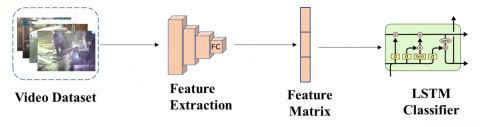
Figure 4. Video classification algorithm
In Figure 4 we see a video classification algorithm. First of all, the frames of the videos belonging to each of the 4 classes we have are arranged one after the other. Consecutive frames are sent to a pre-training algorithm so that their features can be extracted. The obtained features are classified in MATLAB by sending them to the LSTM classifier. The LSTM classifier is used because it is a time-dependent classifier. Thus, it is a widely used algorithm for the classification of video in close pattern with time information.
Video Classification Algorithm
Start
Step-0: Loading Dataset
Loading Anomaly-Detection-Dataset-UCF dataset
Create feature Matrix
Choose the feature extraction type (Alexnet or Vgg19 or Resnet18)
Step-1: Feature Extraction
Extract features from the pre-training algorithm with transfer learning
Obtain Alexnet or Vgg19 or Resnet18 feature matrix
Step 2: Divide Data with K-Fold Cross Validation
Divide the Feature matrix into 5-folds
Step-3: Train LSTM Classifier
send all data in series to the LSTM classifier
all attributes are from the Gaussian distribution
Step-4: Classify Test Data Classify test data with 5 folds using the LSTM model
Used to classify time-dependent and tri-door LSTM models
Step-5: Calculate Test Performance
Achieve scores in accuracy, precision, recall, F1 scores
With 5 folds the average accuracy performance is calculated
End
3 different pre-training algorithms were taken into the re-training process, allowing us to obtain 1500 features for each frame. It is possible to obtain any number of features with this method 3 of them.
The results obtained were compared by classifying the features obtained from 3 different pre-training algorithms separately for 4-class video data, one of which was related to events involving criminal elements and undesirable situations, and one of which was from normal daily events. These 3 pre-training algorithms; Alexnet, Vgg19, Resnet18.
While 1500 features were obtained from the fully connected layer for Alexnet, Vgg19, and Resnet18, after the features were obtained, the classification step for each algorithm was done in 5 folds. The reason for the classification 5-fold is to review all the data and to reach accurate results by preventing coincidental results. Because cross-validation is necessary to obtain reliable and more accurate results. In each cycle, test and training data are randomly divided and this is done 5 times [20].
Based on all this, let's examine some calculations used in classifying videos. Machine learning studies; The limits obtained for the criteria of the model used are used in the evaluation results in a matrix format called the error matrix (confusion matrix), which is an indicator of how close or far the prediction of the targeted attribute values is. According to the results obtained from confusion matrices, the highest accuracy was obtained from Resnet18. Resnet18 has a higher number of layers than the other 2 networks. In terms of depth, it is almost the same depth as Vgg 19. Batch normalization layers have been shown to affect accuracy. vgg 19 is equivalent to resnet18 in terms of both depth and number of relu layers. It has more pooling layers. but the number of layers is less. this appears to have some negative impact on accuracy. Alexnet, on the other hand, has fewer layers and less depth than both algorithms. As a result, it was determined that there was a decrease in test accuracy.
The performance of the model [11], which is generally used in machine learning studies, is evaluated using the evaluation results in the form of a matrix called the confusion matrix, which is an indicator of how close or far the feature matrices are with the real values. The confusion matrix shows how well the predicted values fit the target values. congruent values are located in the diagonal section. An example error matrix for the simplest two-class classification problem is shown in Table 1. These parameters are used to evaluate error matrices with two or more classes: True Positive (TP), False Positive (FP), True Negative (TN), and False Negative (FN), each of which will be described below. Examining the parameters in the table, Accuracy Rate is a measure of how accurate the classifier's predictions are, while Error Rate is a measure of how incorrect the Classifier's predictions are, and therefore a low "error rate" is desired. that is, the accuracy rate and the error rate are inversely proportional. The recall is a measure of how accurately you guessed from tests labeled as positive and intended to be as high as possible. Precision, when analyzed, is a measure of how accurately positive predictions are made and is also a measure of performance appraisal that is intended to be large.
Figure 5 refers to the confusion matrices obtained by classifying Alexnet, vgg19 and resnet18 pre-training algorithms into 5 folds after the transfer learning process. It is seen that the accuracies are proportional to each other and the values in the matrices are distributed homogeneously. This reveals that a sufficient amount of information is classified.
Table 1. Basic explanation of the confusion matrix
|
Positive |
Negative |
|
TP |
FP |
|
FN |
TN |
(a)
(b)
(c)
Figure 5. Truth matrices of three different algorithms (a) Alexnet confusion matrix(b) Vgg19 confusion matrix (c) Resnet18 confusion matrix
The desired situation is a result of the evaluation obtained in this way; The aim is to ensure that the sizes on the main diagonal are as large as possible by using a correctly constructed model (in this study, the appropriately selected feature and classifier pair). Especially when all the cells in this matrix are normalized by dividing by the relevant "target sample" numbers in the data set, it is possible to evaluate the model performance visually easily.
TP: In fact, the feature labeled as positive was also predicted positively by the algorithm.
TN: In fact, a feature labeled as negative is also predicted negatively by the algorithm.
FP: An attribute that was originally labeled as negative was incorrectly predicted as positive by the algorithm.
FN: An attribute that is positively labeled is mistakenly predicted as negative by the algorithm.
Accuracy Rate: The accuracy of the predictions made by the classifier can be adjusted in advance. Figure 6 shows the classification accuracies obtained for all three pre-training algorithms. The accuracies were obtained from the confusion matrix with the help of formula 1. And for the three pre-training algorithms are shown comparatively in the column chart.
(TP+TN)/Total Number of Samples (1)
Figure 6. Accuracy of Alexnet, Vgg19, Resnet18 algorithm
Error Rate: It is a measure of how wrong the classifier's predictions are, in percent, and the accuracy is expected to be low, on the contrary. It is defined by Eq. (1) as follows. Based on the classification accuracies, error rates were obtained. and were compared with each other in Figure 7, with the help of the accuracies given by the features obtained as a result of the three pre-training algorithms. It has been observed that the error rate for Resnet18 is very low and the convolution layers have positive effects on classification.
(FP+FN)/Total Number of Samples (2)
Figure 7. Error rates of Alexnet, Vgg19, Resnet18 algorithm
Recall: This value is also a measure of how accurately the positively labeled features are predicted, and this is intended to be as high as possible. The true positive value is equal to the sum of the true positive and false negative values. Sensitivity value is also a measurement that will help us since it is costly to predict False Negative. It should be as high as possible. This metric is defined as follows:
TP/(TP+FN) (3)
Precision: It is a measure of the accuracy of positive estimates in classification and is a performance evaluation parameter that is intended to be large. It is the ratio of true positive to the sum of true positive and false positive. Precision value is very important, especially when the cost of False Positive prediction is high. For example, if your model marks the e-mails that should arrive in your e-mail inbox as spam (FP), you will not be able to see the important e-mails that you need to receive and you will suffer losses. situation. In this case, a high Sensitivity value is an important criterion for us in model selection.
TP/(TP+FP) (4)
F1-Score: It is the harmonic average of the recall and precision values. this value should also be high. because it contains both precision and callback parameters. The main reason for using the F1 Score value instead of accuracy is to avoid making the wrong model choice in unevenly distributed data sets. Also, the F1 Score is very important to us because we need a measurement metric that includes all error costs.
2×Recall×Presicion/Recall+Presicion (5)
For each class from the confusion matrices obtained as a result of classifying the re-trained alexnet, vgg19, resnet18 pre-training algorithms with 5 folds, recall, precision and F1-score values were calculated one by one with the help of formula 3, 4, 5 and Figures 8-10. It is expressed with column charts in.
Figure 8. Recall, precision, F1 score results for Alexnet architecture
Figure 9. Recall, precision, F1 score results for Vgg19 architecture
Figure 10. Recall, precision, F1 score results for Resnet18 architecture
3.1 Feature distribution histograms of algorithms
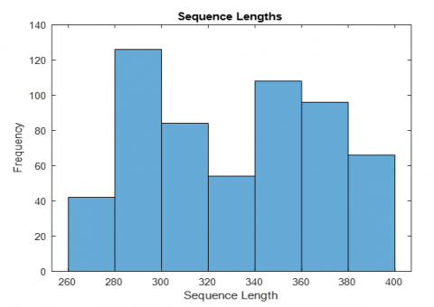
Sending too many attributes to the classification network means adding too much padding. Adding too much padding will adversely affect accuracy and result in lower desired classification results. In this study, it is emphasized that the attributes sent should be at a certain rate. In this way, much more accurate information was obtained. The ratio of the features submitted is poured into a histogram. Thus, it prevents a large amount of attributes from being sent to classification at once. The Histogram information of the feature series sent for classification is shown below [21]. The dimensions of the attributes sent to the system directly affect the result to be obtained, and the parameters such as color, saturation, and saturation of the frames are other factors that directly affect the system's accuracy. Below are the orientation histograms of size 1*576.
Figure 11 shows the feature distribution histograms. For all three algorithms, feature series are grouped between 260 and 400 before being sent to the LSTM network. Thus, more data than the desired rate will not be sent to the network. Based on this; Distribution histograms are visual expressions of the quantities of feature series.
(a)
(b)
(c)
Figure 11. Graph representing the size of the attributes being sent to the network. Exclusion from the than 400. (a) Alexnet feature distribution histogram (b)Vgg19 feature distribution histogram (c) Resnet18 feature distribution histogram
The number of video archives is increasing over time. Therefore, the existence of the internet and technological innovations make video sharing easier. With a simple click on any smart device, a video can be captured and shared with the world [18]. However, it may be difficult to learn what the features of these videos are and to distinguish the content of the captured video. Artificial intelligence helps us analyze videos, extract their features, and ultimately classify them [22]. This classification process is done with ML algorithms. But there is a lot of information in this area. It is necessary to distinguish this information and use it correctly [23, 24]. This problem is overcome by machine learning. The most important advantage of ML is that it can automatically extract and distinguish the desired features from high-dimensional data in complex, high-dimensional feature matrices in the desired size. [25, 26]. A video file consists of a series of image frames, and all frames contain detailed features of that video. However, the important parameter regarding the features to be obtained is from which part of the image and how many features will be extracted from each frame. As the number of features retrieved increases, the information obtained about that video will also increase, and therefore the more accurate the classification process will be. Additionally, the extracted features can be pulled from any layer we want, depending on the operation we will perform. But it would be better to extract the features from the last layers. Because the most accurate data can be accessed by going through all deep layers. Thus, high-level features will enter the classifier. Another advantageous situation is to send the obtained features by dividing them into certain proportions instead of sending them to the classifier all at once. This process prevents all data from being sent to the network at the same time. In other words, dividing and classifying the data into parts instead of sending the entire data at once will prevent the data from being memorized. More accurate results are obtained by classifying all the information obtained. To classify the 4-class video dataset, the accuracies of the features obtained with Alexnet, vgg19, and Resnet18 architectures were compared with the LSTM classifier at 5-fold (cross-validation). Cross Validation; It is a technique used to predict how the performance of a model obtained with training data will be with real-world data. This technique; While training the model with training data, evaluates the performance of the model using the remaining data (validation data). In this way; One gets a more accurate idea of how the model will perform with real-world data. Thus, a more accurate classification is made. Additionally, when the test accuracies obtained are examined, it is seen that there is no big difference between the accuracies obtained from all algorithms, but the greatest accuracy is obtained from the Resnet18 architecture. Resnet18 gave 98.5% accuracy, vgg19 gave 96% accuracy, and Alexnet gave 94.3% accuracy. However, it was observed that the difference between the accuracies obtained with the 3 algorithms and the relevant parameters was approximately 2%. This shows that the results are stable.
The reasons for the differences between the accuracy of the algorithms are the number of layers in the algorithm, as well as the depth of the network, the number of features drawn from the network, and the regions where the features are drawn, which are the main factors affecting accuracy. Additionally, results, including specific results such as recall, precision, f1-score, etc., were extracted by calculating the analysis from the confusion matrix. Based on all the results, both transfer learning and cross-validation were used with 3 different pre-training algorithms and the results were compared. In other words, the results of transfer learning and cross-validation in different pre-training algorithms were monitored. It has been determined that there is a relationship between the layers and depth of the network and the accuracies obtained by increasing the number of features. Based on this, it becomes clear that future studies with more advanced, different pre-training algorithms, videos with larger capacities, and more classes may yield more successful results.
A total of 250 videos in mp4 format were used in the study. each contains different frame numbers. In all videos, 1500 features were obtained for each frame from the fully connected layer with transfer learning for each pre-training algorithm. These features were classified with the LSTM classifier in MATLAB. The results of different pre-training algorithms were obtained through the deep learning process. At this point, it was requested to observe the positive and negative effects of the algorithm on classification before training. The first layers contain low-level features, while the last layers contain detailed information. This parameter was taken into account when obtaining properties. Taking features from the last layer (high-level features) positively affects the results obtained. It is aimed to capture more features to increase accuracy by changing the layers containing high-level features.
While Alexnet gave the lowest result with 94.3%, vgg 19 gave the result of 96% and resnet18 gave a result of 98.5%. It was concluded that precision, recall, F1 score, and specificity results were directly proportional to the accuracy obtained. All results obtained from the confusion matrix obtained as a result of the 5-fold classification were calculated separately for each class and average results were obtained. In addition, histograms of the feature matrices included in the classification were extracted and the amount of feature series sent to the classification was kept at a certain rate to prevent overfitting. In this way, it was possible to reach results without memorizing the data.
[1] Wang, J., Ji, J., Ravikumar, A.P., Savarese, S., Brandt, A.R. (2022). VideoGasNet: Deep learning for natural gas methane leak classification using an infrared camera. Energy, 238: 121516. https://doi.org/10.1016/j.energy.2021.121516
[2] Alippi, C., Polycarpou, M.M., Panayiotou, C., Ellinas, G. (2009). Artificial Neural Networks–ICANN 2009. In 19th International Conference, Limassol, Cyprus. https://doi.org/10.1007/978-3-642-04277-5
[3] Sun, J., Wang, J., Yeh, T.C. (2017). Video understanding: From video classification to captioning. Computer vision and pattern recognition. Stanford University, 1-9.
[4] Hamylton, S.M., Morris, R.H., Carvalho, R.C., Roder, N., Barlow, P., Mills, K., Wang, L. (2020). Evaluating techniques for mapping island vegetation from unmanned aerial vehicle (UAV) images: Pixel classification, visual interpretation and machine learning approaches. International Journal of Applied Earth Observation and Geoinformation, 89: 102085. https://doi.org/10.1016/j.jag.2020.102085
[5] Budiharto, W., Andreas, V., Gunawan, A.A.S. (2020). Deep learning-based question answering system for intelligent humanoid robot. Journal of Big Data, 7(1): 1-10. https://doi.org/10.1186/s40537-020-00341-6
[6] Atila, Ü., Sabaz, F. (2022). Turkish lip-reading using Bi-LSTM and deep learning models. Engineering Science and Technology, An International Journal, 35: 101206. https://doi.org/10.1016/j.jestch.2022.101206
[7] Çınar, A., Şenler Yıldırım, Ş. (2022). A hybrid deep learning based classification for some basic movements in physical rehabilitation. NWSA Academic Journals, 17(2): 9-20. https://doi.org/10.12739/nwsa.2022.17.2.1a0478
[8] Hussain, A., Hussain, T., Ullah, W., Baik, S.W. (2022). Vision transformer and deep sequence learning for human activity recognition in surveillance videos. Computational Intelligence and Neuroscience, 2022: 3454167. https://doi.org/10.1155/2022/3454167
[9] Tora, M.R., Chen, J., Little, J.J. (2017). Classification of puck possession events in ice hockey. In IEEE Computer Society Conference on Computer Vision and Pattern Recognition Workshops, pp. 147-154. https://doi.org/10.1109/CVPRW.2017.24
[10] Abdullah, M.U., Alkan, A. (2022). A comparative approach for facial expression recognition in higher education using hybrid-deep learning from students’ facial images. Traitement Du Signal, 39(6): 1929-1941. https://doi.org/10.18280/ts.390605
[11] Stephan, A., Kougia, V., Roth, B. (2022). Sepll: Separating latent class labels from weak supervision noise. arXiv preprint arXiv:2210.13898. https://arxiv.org/abs/2210.13898.
[12] van Houdt, G., Mosquera, C., Nápoles, G. (2020). A review on the long short-term memory model. Artificial Intelligence Review, 53(8): 5929-5955. https://doi.org/10.1007/s10462-020-09838-1
[13] Graves, A., Mohamed, A.R., Hinton, G. (2013). Speech recognition with deep recurrent neural networks. In 2013 IEEE International Conference on Acoustics, Speech and Signal Processing, Vancouver, BC, Canada, pp. 6645-6649. https://doi.org/10.1109/ICASSP.2013.6638947
[14] Fernández, S., Graves, A., Schmidhuber, J. (2007). An application of recurrent neural networks to discriminative keyword spotting. Artificial Neural Networks – ICANN 2007, pp. 220-229. https://doi.org/10.1007/978-3-540-74695-9_23
[15] Li, A., Yuan, M., Zheng, C., Li, X. (2020). Speech enhancement using progressive learning-based convolutional recurrent neural network. Applied Acoustics, 166: 107347. https://doi.org/10.1016/j.apacoust.2020.107347
[16] Raj, H., Weihong, Y., Banbhrani, S.K., Dino, S.P. (2018). LSTM based short message service (SMS) modeling for spam classification. In Proceedings of the 2018 International Conference on Machine Learning Technologies, pp. 76-80. https://doi.org/10.1145/3231884.3231895
[17] Lee, J.H., Han, S.S., Kim, Y.H., Lee, C., Kim, I. (2020). Application of a fully deep convolutional neural network to the automation of tooth segmentation on panoramic radiographs. Oral Surgery, Oral Medicine, Oral Pathology and Oral Radiology, 129(6): 635-642. https://doi.org/10.1016/j.oooo.2019.11.007
[18] Shi, J., Tripp, B., Shea-Brown, E., Mihalas, S., Buice, M.A. (2022). MouseNet: A biologically constrained convolutional neural network model for the mouse visual cortex. PLoS Computational Biology, 18(9): e1010427. https://doi.org/10.1371/journal.pcbi.1010427
[19] Kuncan, F., Kaya, Y., Tekin, R., Kuncan, M. (2022). A new approach for physical human activity recognition based on co-occurrence matrices. Journal of Supercomputing, 78(1): 1048-1070. https://doi.org/10.1007/s11227-021-03921-2
[20] Du, Z., Zhang, G., Lu, W., Zhao, T., Wu, P. (2022). Spatio-temporal transformer for online video understanding. Journal of Physics: Conference Series, 2171(1): 012020. https://doi.org/10.1088/1742-6596/2171/1/012020
[21] Russakovsky, O., Deng, J., Su, H., Krause, J., Satheesh, S., Ma, S., Huang, Z., Karpathy, A., Khosla, A., Bernstein, M., Berg, A.C., Li, F.F. (2015). ImageNet large scale visual recognition challenge. International Journal of Computer Vision, 115(3): 211-252. https://doi.org/10.1007/s11263-015-0816-y
[22] Ibrahim, Z.A.A., Haidar, S., Sbeity, I. (2019). Large-scale text-based video classification using contextual features. European Journal of Electrical Engineering and Computer Science, 3(2). https://doi.org/10.24018/ejece.2019.3.2.68
[23] Schmidhuber, J. (2015). Deep learning in neural networks: An overview. Neural networks, 61: 85-117. https://doi.org/10.1016/j.neunet.2014.09.003
[24] Wu, Z., Jiang, H., Zhao, K., Li, X. (2020). An adaptive deep transfer learning method for bearing fault diagnosis. Measurement, 151: 107227. https://doi.org/10.1016/j.measurement.2019.107227
[25] Shao, H., Jiang, H., Zhang, H., Liang, T. (2018). Electric locomotive bearing fault diagnosis using a novel convolutional deep belief network. IEEE Transactions on Industrial Electronics, 65(3): 2727-2736. https://doi.org/10.1109/TIE.2017.2745473
[26] Qiao, H., Wang, T., Wang, P., Qiao, S., Zhang, L. (2018). A time-distributed spatiotemporal feature learning method for machine health monitoring with multi-sensor time series. Sensors (Switzerland), 18(9): 2932. https://doi.org/10.3390/s18092932