Medikonda Neelima*![]() | I Santi Prabha
| I Santi Prabha![]()
© 2024 The authors. This article is published by IIETA and is licensed under the CC BY 4.0 license (http://creativecommons.org/licenses/by/4.0/).
OPEN ACCESS
The objective of this work develops an Automatic Speaker Verification (ASV) system to discern genuine from spoof speech samples. The speech sample features are extracted using Mel-frequency Cepstral Coefficients (MFCC), Constant Q Cepstral Coefficients (CQCC), and Spectrogram feature extraction techniques. MFCC, CQCC, and Spectrogram feature extraction are the most common feature extraction techniques in detecting spoofs in voice samples. However, for detecting voice spoofing using these techniques there is a requirement to improve the accuracy. To improve the accuracy a novel hybrid feature extraction technique is proposed. In this present work, the hybrid features are generated by combining relevant features from the three mentioned feature extraction techniques. These extracted features of the speech samples are fed to the new fused Convolution Neural Network (CNN) model and LSTM Neural Network to improve the performance of the overall system. The data set for evaluating the system is split into training and testing samples. New CNN with LSTM model trains training samples. After completing the training phase, the model is evaluated for testing samples. This work aims to extract the features using all three mentioned and also the generated hybrid feature extraction techniques. The performance of the new CNN with the LSTM model is evaluated through a confusion matrix and ROC curve. Comparing one among all feature extraction techniques, the generated hybrid feature extraction technique provides a better test accuracy of 98.48% and a low Equal Error Rate (EER) of 2.2%. In the end, the new CNN-LSTM architecture achieved the lowest EER among all feature extraction techniques thanks to the hybrid feature extraction approach.
convolutional neural network (CNN), constant Q cepstral coefficients (CQCC), hybrid feature extraction, long short-term memory (LSTM), Mel-frequency cepstral coefficients (MFCC), spectrogram
An ASV system is a technology that employs an individual’s distinctive vocal traits to confirm their identity. ASV systems enhance the security in various applications, including access control and voice-based authentication. Safeguarding ASV systems against spoofing attacks is a critical concern within the realm of biometric authentication. The perpetuation of spoofing attacks, such as replay attacks [1], speech synthesis [2], voice conversion [3], and impersonation [4], constitutes various methods for generating counterfeit speech. To mitigate the risks associated with spoofing attacks, it is essential to create a system capable of distinguishing between authentic and counterfeit signals. In order to achieve superior performance, Convolutional Neural Networks (CNN) are widely utilized in tasks like video classification, image classification, facial recognition [5], and speech recognition [6].
ASV systems are utilized to authenticate people in a diversity of applications including call centers, banks, smartphones, etc. When considering spoofing attacks ASV systems are more sensitive. In a successful attempt, unauthorized access can be granted to sensitive and private data by a spoofing attack.
Different research works are done to improve the detection rate of ASV systems [7-13]. They used Gaussian Mixture Model (GMM), CNN, and Recurrent Neural Network (RNN) for classifying spoof and genuine samples from the given dataset. Also utilized LFCC and LPCC techniques for feature extraction. However, these systems lack accuracy and reduce errors. So a hybrid feature extraction technique and an ensemble model that combines CNN and Long Short-Term Memory (LSTM) is proposed in the current paper.
The objective of the proposed work is to develop an ensemble model using a hybrid feature extraction technique and CNN-LSTM, to detect the spoof in the given data with more accuracy.
This is achieved by the following contributions as:
(1) Select a dataset suitable for spoof detection. For this work, ASVspoof 2019 dataset is selected, due to the availability of genuine and spoof samples. Also, this dataset contains samples from replay, speech synthesis, and voice conversion attacks which are the possible attacks for the ASV system.
(2) Develop a hybrid feature extraction technique.
(3) Select a suitable classification model.
(4) Evaluate the model using performance metrics.
The related recent works and the issues in those works are given in section two. For tracking these issues, a novel solution is given in section three. Different evaluation metrics for assessing the system’s performance are given in section four. The outcomes obtained by the proposed model are given in section five. A research comparison is given in section six. The conclusion of the research proposal and future directions are given in section seven.
Ensuring the security and authenticity of voice-based systems necessitates the important task of voice spoofing detection. CNN and RNN are some deep learning frameworks, that have proven to be highly effective in this regard [7]. In particular, the combination of CNN and RNN models has demonstrated improved system robustness [8].
In a study conducted by Khan et al. [9], it was observed that the CNN classifier achieved a significantly lower EER compared to the GMM classifier when utilizing the same feature set. For voice spoofing detection, linear-based features like LFCC and LPCC performed well in conjunction with the CNN-based classifier [9].
Another method for voice spoofing detection involves the utilization of LSTM networks. Wang et al. [10] projected an LSTM-based approach for detecting spoofing attacks in the ADS-B protocol. This involved preprocessing the message sequence using a sliding window and training an LSTM network for prediction. Subsequently, the residuum set of true values and expected values was measured to detect spoofing attacks [10].
Deep learning models can also be employed to detect voice replay attacks, a type of voice spoofing attack. Zhou et al. [11] proposed a system that used Linear Frequency Residual Cepstral Coefficient (LFCC) as the feature and employed both CNN and GMM classifiers to differentiate between genuine and replayed audio samples.
Furthermore, a hybrid CNN-LSTM model has been utilized for voice spoofing countermeasures, demonstrating higher accuracy in both the frequency and time domains [12]. In the context of keyword recognition, voice conversion (VC) techniques have been employed to augment limited training datasets. Wubet and Lian [13] proposed a fusion of LSTM and CNN models for robust keyword recognition in speaker-independent scenarios, leveraging voice conversion to generate new voices for training. Overall, deep learning frameworks such as CNN, RNN, and LSTM exhibit promise in voice spoofing detection, enabling effective analysis of acoustic features and differentiation between genuine and spoofed voice signals. The selection of specific models and features depends on the application and the types of targeted spoofing attacks.
Novel characteristics are necessary to tackle compression and encoding-induced artifacts in ASV Systems. The latest ASV challenge, ASVspoof2021, places significant emphasis on countering voice spoofing, particularly about artifacts caused by compression and encoding. These artifacts can significantly impact an ASV system's performance and hinder its ability to accurately detect fraudulent speech. This underscores the importance of continuous research and the imperative for advancements in the field of speech spoofing detection. As attackers employ increasingly intricate and imaginative tactics to exploit ASV systems, researchers must step up to confront the challenge. A comparison of these techniques is given in Table 1.
Table 1. Comparison of related research works
|
Technique |
Advantages |
Use Cases |
Reference |
|
CNN |
Effective for voice spoofing detection |
Low Equal Error Rate (EER) |
Khan et al. [9] |
|
CNN |
Improved system robustness |
Linear based features (LFCC, LPCC) |
Khan et al. [9] |
|
RNN |
Effective for voice spoofing detection |
General voice spoofing detection |
Khan et al. [9] |
|
RNN |
Combining CNN and RNN improves robustness |
Various types of spoofing attacks |
Khan et al. [9] |
|
LSTM |
Effective for voice spoofing detection |
Detection of spoofing attacks |
Wang et al. [10] |
|
CNN+GMM |
Differentiate between genuine and replayed audio samples |
Voice replay attack detection |
Zhou et al. [11] |
|
CNN-LSTM |
High accuracy in frequency and time domains |
Voice spoofing countermeasures |
Mohammed Alsumaidaee et al. [12] |
|
LSTM+CNN |
Robust keyword recognition in speaker independent scenario |
Keyword recognition with limited training data |
Wubet and Lian [13] |
To achieve the required objective and enhance the resilience of ASV systems against spoofing attacks, innovative features, and countermeasures need to be specifically designed.
In real-world scenarios, the acoustic environment can exhibit significant variations, including the presence of background noise, channel distortions, and non-stationary conditions. The challenges posed by these variations can render existing classifiers and feature extraction methods insufficiently robust, leading to the potential for errors and false acceptances or rejections within the ASV system. Many conventional ASV systems typically depend on classical classifiers such as GMMs and Support Vector Machines (SVMs), which may not effectively capture complex speech patterns. More contemporary techniques, such as CNNs, Deep Neural Networks (DNNs), and Recurrent Neural Networks (RNNs) have shown their capability to deliver superior performance in capturing intricate speech patterns. The process of feature extraction plays a pivotal role in representing speech data in a manner conducive to classification. Traditional methods like MFCC may fail to encompass all the pertinent information present in speech signals.
The gaps in the discussed related work are to use of a robust classifier and a suitable feature extraction technique for improving the performance of the ASV system.
Hence on these findings, the ensemble model with optimized features in voice spoof detection is proposed for solving the problems in existing models and discussed in the following sections.
The objective of the proposed work is to develop an ensemble model using a hybrid feature extraction technique and CNN-LSTM, to detect the spoof in the given data with more accuracy.
CNNs excel in the acquisition of hierarchical features from unprocessed data, like audio signal spectrograms. These networks have the capacity to grasp both local and global data patterns. When integrated with Long Short-Term Memory (LSTM) layers, known for their proficiency in modeling temporal relationships, the resulting model becomes adept at acquiring and incorporating spectral and temporal details from audio signals. This integration enhances the system’s capability to generate more distinctive feature representations for speaker verification.
A neural network (NN) based model is used to work with the high-dimensional features for the detection of elaborate information. The genuine and spoof sample features are extracted using magnitude-based features such as MFCC [14], CQCC, and other features such as spectrogram.
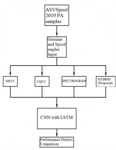
Figure 1. Proposed model architecture
The new hybrid features are generated by combining the most relevant features in the mentioned three feature extraction techniques. Both genuine and spoof sample features are given to the new CNN-LSTM model. Thereby a confusion matrix is derived which summarizes the performance of classification i.e., a table often used to express the execution of a classification framework. Then the Receiver Operating Characteristics (ROC) curve is obtained which is a graph showing the classification model’s performance by comparing the true positive rate and false positive rate. In the present work, the new CNN-LSTM model’s performance is compared when the model is trained with different feature extraction techniques. The speech sample’s features are extracted using MFCC, CQCC, Spectrogram, and Hybrid techniques. The features extracted are supplied to the new CNN-LSTM classifier for classifying them as genuine or spoof. Based on the performance of the new CNN-LSTM for different feature extraction techniques, the best one is stated. The proposed model architecture is given in Figure 1.
3.1 Dataset
This work is carried out on Voice Conversion (VC), Speech Synthesis (SS), and replay attack samples, i.e., ASVspoof 2019 database LA and PA samples. It contains two classes such as genuine and spoof. Each speech sample is approximately 30 seconds of a track.
3.2 Feature extraction
Feature extraction is the technique of creating temporary features from minor depictions using specialist comprehension of unvarying classes. Effective feature extraction techniques create features that have strong discriminatory power. They should be able to distinguish between different classes or categories in the data. Techniques that capture key differences between classes are more likely to perform well.
Feature extraction is associated with dimensional reduction. In this current work, four feature extraction techniques are used. These are MFCC, CQCC, Spectrogram, and Hybrid techniques.
The most common and straightforward approach for extracting spectral and phonetic features from human speech is through the use of MFCC. Constant Q Cepstral Coefficients (CQCC) are a set of features commonly used in audio signal processing for their effectiveness in capturing pitch-related characteristics of sound, making them valuable for tasks like music analysis and speech recognition. Spectrogram feature extraction involves the conversion of audio signals into a visual representation that displays how the signal’s frequency content evolves over time, making it a valuable technique for tasks such as sound analysis, speech processing, and music recognition.
3.2.1 Mel-frequency cepstral coefficients (MFCC)
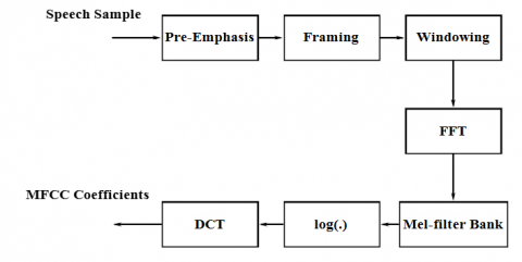
Figure 2. Procedural steps of MFCC feature extraction
The easiest and most prevalent method to extract spectral and phonetic features from the human voice is MFCC [15]. This is one of the most outstanding methods of extracting speech sample features used in speech recognition systems [16, 17]. It is based on the frequency domain in the Mel scale which relies on the human ear scale. This technique extracts the features that are the same as changes in the human ear cochlea’s critical bandwidth with frequency [18]. The procedural steps involved in MFCC are given in Figure 2.
Pre-emphasis. Most of the speech signal’s energy is concentrated on higher frequencies than on lower frequencies. So to improve the higher frequency component’s energy, the sample is passed through a pre-emphasis filter.
Frame blocking. A speech signal is a non-stationary signal. However, the speech signal’s small duration segment is stationary. So speech sample is fragmented into short segments of twenty to thirty milliseconds in duration. These are called frames. Hence, short-time spectral analysis is preferred in this stage to split the speech sample into small duration segments.
Hamming windowing. To keep the progression in the signal, every frame is processed with a Hamming window. Hamming window smoothly tapers at the edges which causes energy loss in the speech frames at the edges. To avoid this an overlapped Hamming window of five milliseconds is used.
Fast Fourier Transform. FFT is a process to get frequency components from a time domain signal. A spectrum is obtained when FFT is applied to the windowed frame.
Triangular band-pass filters. To get a smooth magnitude spectrum in the mel scale, the magnitude of the frequency spectrum obtained from the previous step is multiplied by twenty triangular band-pass filters. The size of features is also reduced by this step.
$Mel(f)=1125*\ln \left( 1+\frac{f}{700} \right)$ (1)
where, Eq. (1) describes the conversion from frequency f to mel.
Discrete Cosine Transform. Energy derived from previous bandpass filter is given to discrete cosine transform after converting to db scale. There by L mel-scale cepstral coefficients are obtained as given in Eq. (2).
$\mathop{c}_{m}=\sum\limits_{k=1}^{N}{\log \left( \mathop{E}_{k} \right)\left( \cos \left( 2m\left( k-0.5 \right)\frac{\pi }{N} \right) \right)},m=1,2,...L$ (2)
where, cm: MFCC coefficients for the mth sample; N: number of mel filter banks; Ek: energy in the k-th mel filter; L: number of samples.
Discrete Cosine Transform (DCT) is applied on the log mel spectrum to convert it back into the time domain.
Delta cepstrum. The components c0 is the power of all frequency components and c1 is compatibility among lower and higher-frequency components inside a frame. The remaining cepstral coefficients do not have reasonable consideration. They include finer details of the spectrum to differentiate sounds [18].
3.2.2 Constant Q cepstral coefficients (CQCC)
CQCC is particularly efficient in identifying speech synthesis attacks. However, it failed to detect spoof attacks [19].
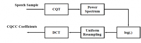
Figure 3. Block diagram of CQCC feature extraction
The procedural steps involved in CQCC [19] are given in Figure 3.
·The speech samples are given to Constant Q Transform (CQT) [20, 21].
·Signal is transferred to the power spectrum where the signal’s absolute value is obtained.
·Now the logarithmic function is applied to the signal which comes from the power spectrum.
·Then the logarithmic signal gets uniform resampled.
·Lastly, the signal is transferred to components using DCT.
The Q-factor, obtained after CQT is a filter’s exactness measuring factor that reflects the division of mid-frequency to the bandwidth.
The time sequence’s cepstrum is procured by taking the logarithm of the squared magnitude spectrum and applying an inverse transformation to it. A spectrum’s orthogonal decomposition is termed a cepstrum. The output of the uniform resamples module is given to the discrete cosine transform module. So, the logarithmic linear power spectrum is then passed to DCT.
3.2.3 Spectrogram features
A spectrogram shows how the signal strength is distributed in each frequency found in the signal. A Spectrogram is constructed from a series of spectra by stacking them in time and compacting the amplitude axis into a gray line called a “contour map” [22]. Black is used for most energy, while white is used for the least.
Two types of spectrograms are used in the speech signal study. The first type emphasizes the frequency details by utilizing narrow analysis filters or long signal areas, and another type emphasizes the temporal details by utilizing wide analysis filters or short signal sections [23]. Narrow-band spectrograms are advantageous for researching the attributes of the source. For example, the vocal fold vibration’s harmonics are shown. Wide-band spectrograms help examine the qualities of vocal tract filtrate: they feature the vocal tract formants by showing how they keep on vibrating after a vocal fold pulse has gone through. Spectrograms are useful for the evaluation of text-to-speech systems [24]. This work aims at the speaker not on vocal tract filter, so a narrow band spectrogram is selected.
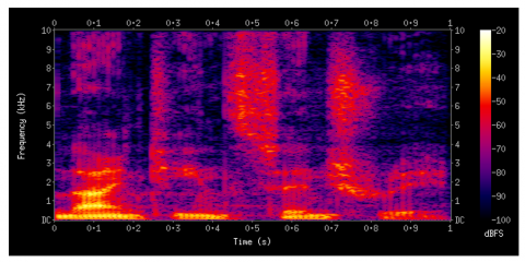
Short-time Fourier Transform. As the frequency and phase of nearby parts of the signal change over time, smaller frames are obtained by dividing the signal, and then the Fourier transform is applied. This process is called the Short-Time Fourier Transform (STFT) [25]. Truly, computing STFTs involves partitioning a larger temporal signal into equivalent-length portions and processing the Fourier transform freely on each more limited section [26]. A spectrogram is then made by plotting the varying spectra as a component of time. A typical spectrogram for one of the training samples from the dataset is given in Figure 4.
Figure 4. Spectrogram of a replay sample from database
On account of continuous-time signals, the information to be changed over is duplicated by a windowing function that is non-zero for a brief period.
In the discrete-time case, information to be changed could be separated into chunks of frames (which for the most part cross over one another, to lessen artifacts at the limit) [27, 28].
Spectrograms [29] are utilized widely in various applications such as speech signal processing, sonar signal processing, music, radar signal processing, linguistics, etc.
Generation of spectrogram. Spectrograms could be obtained from a signal sample in the following ways: using a series of bandpass filters, or computed by the use of Fourier transform [30].
The two techniques make two distinct representations of time-frequency [31] however are identical under specific circumstances. The bandpass filter strategy ordinarily utilizes an analog signal process to separate the input sample into frequency bands. Then the property of the output of each filter stores the spectrogram as a paper image. In the time domain, carefully examined information is partitioned into lumps that by and large crossover, and the frequency spectrum’s magnitude for each piece is calculated using the Fourier transform. Each chunk is then represented as an upward line in the picture, which represents a frequency versus magnitude measured at a certain point in time. These spectra or time plots are then placed one next to the other to make a picture or three-layered surface or marginally covered in different ways, referred to as windowing. The squared magnitude of the short-time Fourier transform (STFT) of a signal is computed by using this process.
3.2.4 Hybrid features
MFCCs are known for their robustness in capturing phonetic information, while CQCCs are effective in capturing pitch-related features. Spectrogram features offer information about the time-frequency representation of the audio signal. The combination of these features can make the model more robust to variations in speech.
By reducing the present multiple features for speech samples to make the classification process easier, hybrid features were generated using Eq. (3):
$\begin{align} & Hybrid\_features=\left[ MFCC\_f,CQCC\_f,SP\_f \right] \\\end{align}$ (3)
where, MFCC_f: MFCC features; CQCC_f: CQCC features; SP_f: Spectrogram features.
The hybrid features were obtained by concatenating the feature vectors from MFCC, CQCC, and spectrogram features. This is done to create a single, combined feature vector that represents the audio data comprehensively with information from all three feature extraction techniques.
During the hybrid features generation process, the considered features were CQT, spectral bandwidth, spectral roll-off, and the mel-frequency features. The remaining undesired features were discarded.
3.3 Convolutional neural network (CNN) model
CNN is a deep learning algorithm, it relegates significance to various partitions of the picture and may separate them from one another [32]. A neural network has at least one convolutional layer and it is utilized basically in image processing, classification, and other autocorrelated information.
The pre-processing expected in a Conv Net is a lot lower contrasted with other classification algorithms. Conv Nets are becoming more familiar with the use of filters. The job of the Conv Net is to lessen the images into a structure that is more straightforward to process, and that is basic to get a decent forecast without losing features.
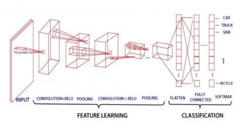
CNN is a numerical build that ordinarily comprises 3 sorts of layers: convolution layer, pooling layer, and fully connected layers which are shown in Figure 5. The first two layers of CNN primarily, the convolution layer and pooling layer are used to extract features from the given speech sample. And third, a fully connected layer is used to map the generated features into the CNN, which comprises numerical tasks, such as convolution and linear operation.
The training dataset is used to apply to the CNN model, and the model is then evaluated for specific kernels with varying weights to calculate the loss function. This is achieved through forward propagation. In this, the weights and kernels are learnable parameters. These parameters are trained through backpropagation using a gradient descent optimization algorithm.
Figure 5. A typical CNN block diagram
Convolutional neural networks exploit the way that the information comprises pictures and they urge the engineering all the more reasonably. Specifically, dissimilar to a standard neural network, the layers of a convolution neural network have neurons organized in 3 aspects: width, height, and depth.
3.3.1 Layers of CNN
Convolution layer. This is the main layer that is utilized to separate the different features from the input images.
Pooling layer. A convolutional layer is generally trailed by a pooling layer. The essential point of this is to decrease the size of the convolved map of features to lessen computational expenses.
Fully connected layer. This layer comprises the biases and weights alongside the neurons and interfacing the neurons between two distinct layers is utilized.
Dropout layer. To dispose of the overfitting problem, a dropout layer is utilized. In the training cycle of neural networks, a few unimportant neurons are discarded by this layer. There a diminished size model is obtained. Twenty-five percent of the nodes are discarded when a dropout factor of 0.25 is used [33].
Activation functions or non-linearity (ReLU). Finally, one of the foremost prominent parameters of the CNN model is the activation function [34]. They are utilized to learn and gauge any sort of continuous and complex connection between variables of the network.
3.4 Learning algorithm
3.4.1 CNN-LSTM with an MFCC model
The features of samples are extricated by utilizing the MFCC feature extraction technique. MFCCs are recognized for their ability to effectively capture phonetic details. In the proposed new CNN with LSTM architecture, initially, five convolution block layers are created. Each block layer contains a convolution kernel with different kernel sizes accompanied by a max-pooling layer and a dropout with a drop rate of 0.25. After that LSTM layer is used and the output is flattened into a 1D array and six dense layers finally, to the last one, the output layer. Initially, the model fits training samples and then the model evaluates the test loss and from which the test accuracy.
3.4.2 CNN-LSTM with a CQCC model
CQCCs excel in capturing features related to pitch. After the completion of loading speech samples, the extraction of CQT cepstral features is done. Then these samples are split into test data and train data. Usually, test data is 30% of the complete data and the rest of the data is train data. After completion of the splitting of data into corresponding sets, it is applied to a new CNN-LSTM classifier and here the classification between the spoof and genuine samples will be done. From which the test loss and the test accuracy for each epoch are calculated and after completion of all epochs, the test loss and test accuracy will be displayed.
3.4.3 CNN-LSTM with a spectrogram model
Spectrogram features provide insights into the time-frequency representation of the audio signal. In this work, the features of samples are extricated by utilizing the spectrogram feature extraction technique. These features are applied to the proposed new CNN with LSTM architecture. Initially, the model fits training samples and then the model evaluates the test loss and from which the test accuracy.
3.4.4 CNN-LSTM with a hybrid model
The features of samples are extricated by utilizing a hybrid feature extraction technique. These features are applied to the proposed new CNN with LSTM architecture. Initially, the model fits training samples and then the model evaluates the test loss and from which the test accuracy.
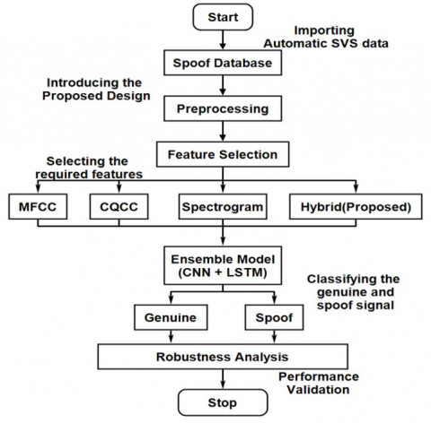
The workflow of the present work is given in Figure 6.
Figure 6. Work flow of ensemble model with hybrid features model
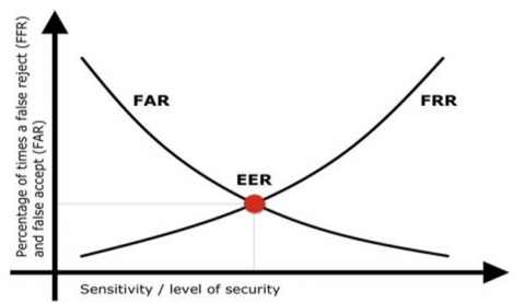
A measurement is utilized to demonstrate biometric execution, regularly while working on a verification task. EER is a value in Receiver Operating Characteristics (ROC) curve, in which the false rejection rate (FRR) and false acceptance rates (FAR) are the same [35].
The biometric system’s accuracy is dependent on EER. If the error margin is less then accuracy will be more. EER is calculated by taking the average between FAR and FRR.
4.2 False acceptance rate (FAR) and false rejection rate (FRR)
FAR is a measurement used to gauge biometric performance while working on the verification task. FAR is the measure of the likelihood that the system incorrectly accepts an access attempt by an unauthorized user. FAR occurs when the system accepts a user where the user ought to have refused. The identification percentage occurs when unapproved people are mistakenly acknowledged. These types of problems are known as false positives.
FRR is the problem of rejecting a legal user when the system should have accepted it. The identification percentage occurs when approved people are erroneously rejected.
The value of the EER can be easily generated from the ROC curve as shown in Figure 7. The EER enables quick comparison of the accuracy of devices with different ROC curves.
Figure 7. Plot of EER
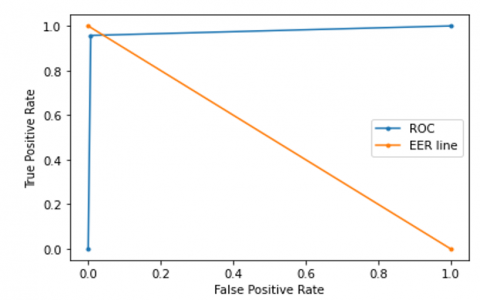
4.3 Receiver operating characteristics (ROC) curve
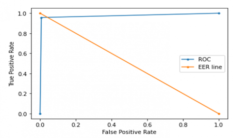
A plot of signal (TPR) against noise (FPR) is known as a ROC curve. Classification metrics of the model’s performance are given by the ROC which is shown in Figure 8.
Figure 8. Plot of ROC
The ROC curve is a measure of evaluating binary classification problems. The ROC curve gives the compromise between sensitivity (or TPR) and specificity (1-FPR).
The Area Under the Curve (AUC) within a ROC plot serves as a metric for assessing the effectiveness of a binary classification model, such as a machine learning classifier. The ROC plot offers a visual depiction of a model’s capacity to differentiate between two classes while modifying the classification threshold. The AUC quantifies the model’s overall performance by measuring the area beneath the ROC curve. An ideal classifier would achieve an AUC of 1, signifying its capability to perfectly distinguish between the two classes. Conversely, an AUC of 0.5 signifies a classifier that performs no better than random chance, as the ROC curve aligns with the diagonal line extending from the bottom-left to the top-right of the plot.
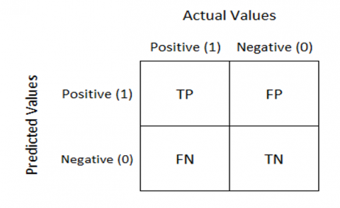
4.4 Confusion matrix
A model confusion matrix is shown in Figure 9.
Figure 9. Confusion matrix
True Positive (TP): It is the total counts having both predicted and actual values are positive.
True Negative(TN): It is the total counts having both predicted and actual values are negative.
False Positive (FP): It is the total counts having prediction is positive while actually negative.
False Negative (FN): It is the total counts having prediction is negative while actually, it is positive.
Using the entities of the confusion matrix, recall, f1 score, precision, and accuracy are determined.
Precision measures the accuracy of positive predictions made by a classification model. It is calculated as the ratio of true positives to the sum of true positives and false positives. It is the positive forecasting outcome, which is formulated in Eq. (4):
$\Pr ecision=\frac{True\_Positives(TP)}{False\_Positives(FP)+True\_Positives(TP)}$ (4)
Recall measures the ability of a classification model to identify all relevant instances in a dataset. It is calculated as the ratio of true positives to the sum of true positives and false negatives. Recall gives the measure of how well a model can identify all relevant instances in an outcome, which is formulated in Eq. (5):
$\operatorname{Re}call=\frac{True\_Positives(TP)}{False\_Negatives(FN)+True\_Positives(TP)}$ (5)
The F1-score is a single metric that combines both precision and recall into a single value. It is particularly useful when there is a need to balance precision and recall. The F1-score is the harmonic mean of precision and recall. F1-score gives the mean robustness rate, which is formulated in Eq. (6):
$F-Score=2*\frac{\Pr ecision\times \operatorname{Re}call}{\Pr ecision+\operatorname{Re}call}$ (6)
Accuracy measures the overall correctness of a classification model. It is calculated as the ratio of the total number of correct predictions (both true positives and true negatives) to the number of predictions. Accuracy gives the measure of exact spoof and genuine detection from the total given samples, which is formulated in Eq. (7):
$Accuracy=\frac{TP+TN}{TP+FN+TN+FP}$ (7)
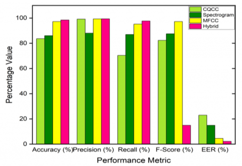
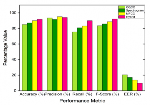
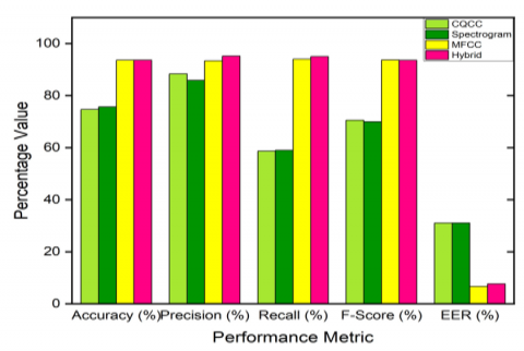
The proposed model CNN with LSTM for different feature extraction techniques is observed through evaluation metrics. The different evaluation parameters of the ensemble model with different features on replay, speech synthesis, and voice conversion attacks are observed and tabulated in table 2, 3, and 4 respectively. From the observations, it is known that the hybrid model is giving outstanding performance compared with other models used in this work. The performance of the hybrid model is shown in Table 5.
Table 2. Performance of ensemble model with different features on replay attack
|
Feature Extraction Technique |
Accuracy (%) |
Precision (%) |
Recall (%) |
F-Score(%) |
EER (%) |
|
CQCC |
83.63 |
99.21 |
70.39 |
82.35 |
22.96 |
|
Spectrogram |
86.06 |
88.04 |
87.01 |
87.56 |
14.92 |
|
MFCC |
97.27 |
99.37 |
95.23 |
97.26 |
4.57 |
|
HYBRID |
98.48 |
99.43 |
97.70 |
98.59 |
2.2 |
Table 3. Performance of ensemble model with different features on speech synthesis attack
|
Feature Extraction Technique |
Accuracy (%) |
Precision (%) |
Recall (%) |
F-Score(%) |
EER (%) |
|
MFCC |
90.00 |
95.16 |
83.09 |
88.72 |
13.65 |
|
CQCC |
85.00 |
93.44 |
75.49 |
83.51 |
20.56 |
|
Spectrogram |
87.00 |
91.47 |
80.82 |
85.81 |
17.11 |
|
HYBRID |
91.66 |
94.11 |
90.00 |
92.01 |
9.65 |
Table 4. Performance of ensemble model with different features on voice conversion attack
|
Feature Extraction Technique |
Accuracy (%) |
Precision (%) |
Recall (%) |
F-Score(%) |
EER (%) |
|
MFCC |
93.66 |
93.42 |
94.03 |
93.72 |
6.66 |
|
CQCC |
74.66 |
88.34 |
58.70 |
70.54 |
31.04 |
|
Spectrogram |
75.66 |
85.85 |
59.02 |
69.95 |
31.04 |
|
HYBRID |
93.67 |
95.20 |
92.05 |
93.60 |
7.69 |
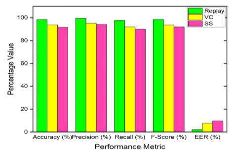
Table 5. Performance of ensemble model with hybrid features on different attacks
|
Attack Type |
Accuracy (%) |
Precision (%) |
Recall (%) |
F-Score(%) |
EER (%) |
|
Replay |
98.48 |
99.43 |
97.70 |
98.59 |
2.20 |
|
VC |
93.67 |
95.20 |
92.05 |
93.60 |
7.69 |
|
SS |
91.66 |
94.11 |
90.00 |
92.01 |
9.65 |
Figure 10. Comparison of various parameters for different feature extraction techniques on replay attack
Figure 11. Comparison of various parameters for different feature extraction techniques on speech synthesis attack
Figure 12. Comparison of various parameters for different feature extraction techniques on voice conversion attack
Figure 13. Comparison of various parameters for hybrid feature extraction technique on different attacks
The comparison between different feature extraction techniques is also shown as a histogram in Figures 10-12 respectively. The performance of the ensemble model with hybrid features on different attacks is shown in Figure 13.
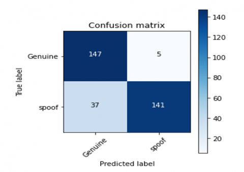
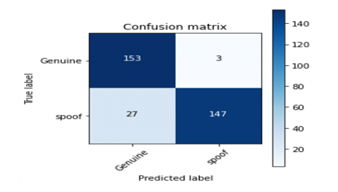
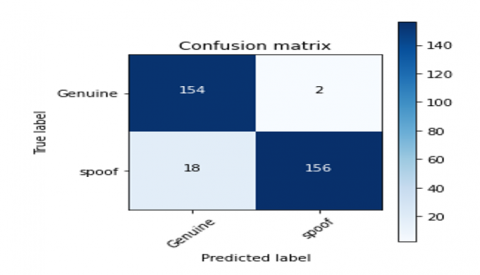
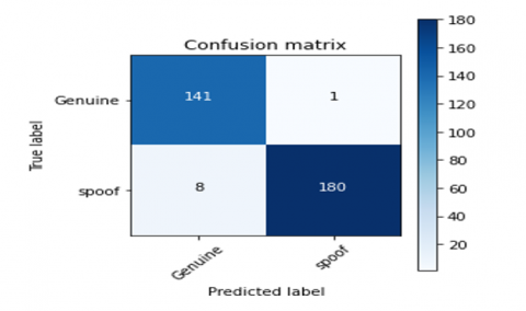
Confusion matrices for different feature extraction techniques for the proposed CNN-LSTM model are derived. The confusion matrix for the CNN-LSTM model with CQCC, Spectrogram, MFCC, and Hybrid feature extraction techniques are shown in Figures 14-17 respectively.
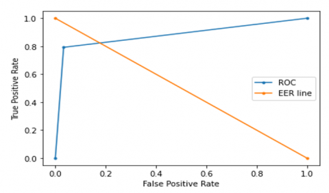
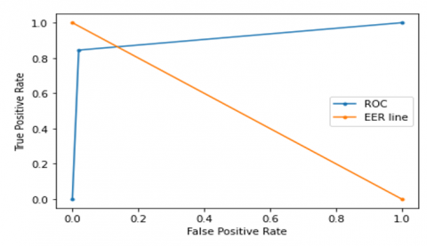
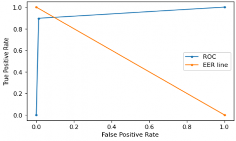
The ROC curve for the CNN-LSTM model with CQCC, Spectrogram, MFCC, and hybrid feature extraction techniques is shown in Figures 18-21 respectively.
Figure 14. Confusion matrix for CQCC CNN-LSTM model
Figure 15. Confusion matrix for spectrogram CNN-LSTM model
Figure 16. Confusion matrix for MFCC CNN-LSTM model
Figure 17. Confusion matrix for hybrid CNN-LSTM model
Figure 18. ROC curve for CQCC CNN-LSTM model
Figure 19. ROC curve for spectrogram CNN-LSTM model
Figure 20. ROC curve for MFCC CNN-LSTM model
Figure 21. ROC curve for hybrid CNN-LSTM model
For evaluating the proposed model, some related existing models were taken, such as Meta-Learning (ML) [36], Attention Neural Model (ANM) [37], Self Attention Framework (SAF) [38], and Bayesian Embedding Model (BEM) [39]. This comparison assessment is given in Table 6. The main performance measures like F-Score, recall, precision, and accuracy are compared. The F-score achieved by the ML system is 87%, recall is 88%, precision is 86%, accuracy is 87.4%, and EER is 12.6. The ANM system achieved an F-Score of 83%, recall of 83.5%, precision of 82.5%, accuracy of 83.4%, and EER of 16.6%. The SAF system achieved a recall of 94%, F-Score of 92.8%, precision of 92.8%, accuracy of 92%, and EER of 8%, whereas the BEM system achieved an F-Score of 91%, recall of 92%, precision of 90%, accuracy of 89.6%, and EER of 10.4%.
In comparison with these models, the proposed and designed model yielded 98.59% F-Score, 97.7% recall, 99.43% precision, 98.48% accuracy, and 2.2% EER.
Our proposed technique exhibits performance similar to that of existing models, with the examination being conducted on the value of EER obtained. Among the various approaches, the baseline using LFCC-GMM is the least effective, yielding an EER value of 13.54%, while the CQCC-GMM approach achieves an EER of 11.04%. Ranked second in effectiveness is [36], which utilizes a Deep Neural Network and CQSPIC method for classifying authentic or replay speech, resulting in an EER value of 7.99%. Another notable approach is [7] with an EER of 6.73%. When compared to these methods, our proposed technique demonstrates outstanding performance, achieving an EER of 2.2%. This significantly lower EER value indicates our approach’s superiority over other techniques. The comprehensive experimental findings, along with the comparison to traditional classifiers, affirm that our proposed approach effectively captures the distinctive features of spoof attacks and authentic audio signals.
Table 6. Comparison of proposed model with existing models
|
Model |
Accuracy (%) |
Precision (%) |
Recall (%) |
F-Score (%) |
EER (%) |
|
ML [36] |
87.4 |
86.0 |
88.0 |
87.0 |
12.6 |
|
ANM [37] |
83.4 |
82.5 |
83.5 |
83.0 |
16.6 |
|
SAF [38] |
92.0 |
92.8 |
94.0 |
92.8 |
8.0 |
|
BEM [39] |
89.6 |
90.0 |
92.0 |
91.0 |
10.4 |
|
Proposed |
98.48 |
99.43 |
97.70 |
98.59 |
2.20 |
The proposed architecture was evaluated based on the ASVSPOOF 2019 samples to detect genuine and spoof speech utterances. The new CNN-LSTM architecture was built on a mixture of MFCC, CQCC, and Spectrogram feature extraction techniques and also to boost the advantages of hybrid features which are the results of integrating different extracted features.
Hybrid feature extraction techniques integrate various feature extraction methods, and their effectiveness depends on their capacity to gather valuable and complementary information from diverse sources. By doing so, this approach boosts system performance by harnessing the advantages of individual techniques, addressing their limitations, and yielding a more extensive and distinctive data representation. Vital attributes that enhance system performance in hybrid feature extraction comprise synergy, merging information, and adaptability to particular tasks, resulting in a more resilient and versatile solution for a wide range of applications.
Eventually, the hybrid feature extraction technique gave the best accuracy and low EER among all feature extraction techniques with the new CNN-LSTM architecture. On comparing with the existing models, the proposed model had given 54% improvement in EER, and 12% improvement in the accuracy by adopting hybrid features.
Although existing ASV systems have gotten significant attention, several challenges must be addressed. The future work is to combine voice recognition with other biometric modalities like facial recognition, fingerprint scanning, etc., for multi-modal biometric systems which can improve security further.
[1] Villalba, J., Lleida, E. (2011). Detecting Replay Attacks from Far-Field Recordings on Speaker Verification Systems. In: Vielhauer, C., Dittmann, J., Drygajlo, A., Juul, N.C., Fairhurst, M.C. (eds) Biometrics and ID Management. BioID 2011. Lecture Notes in Computer Science, vol 6583. Springer, Berlin, Heidelberg. https://doi.org/10.1007/978-3-642-19530-3_25
[2] De Leon, P.L., Pucher, M., Yamagishi, J., Hernaez, I., Saratxaga, I. (2012). Evaluation of speaker verification security and detection of HMM-based synthetic speech. IEEE Transactions on Audio, Speech, and Language Processing, 20(8): 2280-2290. https://doi.org/10.1109/tasl.2012.2201472
[3] Alegre, F., Amehraye, A., Evans, N. (2013). Spoofing countermeasures to protect automatic speaker verification from voice conversion. In 2013 IEEE International Conference on Acoustics, Speech and Signal Processing, Vancouver, BC, Canada, pp. 3068-3072. https://doi.org/10.1109/ICASSP.2013.6638222
[4] Neelima, M., Santiprabha, I. (2020). Mimicry voice detection using convolutional neural networks. In 2020 International Conference on Smart Electronics and Communication (ICOSEC), Trichy, India, pp. 314-318. https://doi.org/10.1109/ICOSEC49089.2020.9215407
[5] Lakshminarasimha, K., Ponniyin Selvan, V. (2022). Deep learning base face anti spoofing -convolutional restricted basis neural network technique. IETE Journal of Research, 69(4): 1-11. https://doi.org/10.1080/03772063.2022.2028583
[6] Padmanabhan, J., Johnson Premkumar, M.J. (2015). Machine learning in automatic speech recognition: A survey. IETE Technical Review, 32(4): 240–251. https://doi.org/10.1080/02564602.2015.1010611
[7] Lavrentyeva, G., Novoselov, S., Malykh, E., Kozlov, A., Kudashev, O., Shchemelinin, V. (2017). Audio replay attack detection with deep learning frameworks. In Interspeech, Stockholm, Sweden, pp. 82-86. http://doi.org/10.21437/Interspeech.2017-360
[8] Guo, J., Zhao, Y., Wang, H. (2023). Generalized spoof detection and incremental algorithm recognition for voice spoofing. Applied Sciences, 13(13): 7773. https://doi.org/10.3390/app13137773
[9] Khan, A., Malik, K.M., Ryan, J., Saravanan, M. (2022). Voice Spoofing Countermeasures: Taxonomy, State-of-the-art, experimental analysis of generalizability, open challenges, and the way forward. arXiv preprint arXiv:2210.00417. https://arxiv.org/abs/2210.00417
[10] Wang, J., Zou, Y., Ding, J. (2020). ADS-B spoofing attack detection method based on LSTM. EURASIP Journal on Wireless Communications and Networking, 2020(1): 1-12. https://doi.org/10.1186/s13638-020-01756-8
[11] Zhou, J., Hai, T., Jawawi, D.N.A., Wang, D., Ibeke, E., Biamba, C. (2022). Voice spoofing countermeasure for voice replay attacks using deep learning. Journal of Cloud Computing Advances Systems and Applications, 11(1): 51. https://doi.org/10.1186/s13677-022-00306-5
[12] Mohammed Alsumaidaee, Y.A., Yaw, C.T., Koh, S.P., Tiong, S.K., Chen, C.P., Yusaf, T., Raj, A.A. (2023). Detection of corona faults in switchgear by using 1D-CNN, LSTM, and 1D-CNN-LSTM methods. Sensors (Basel, Switzerland), 23(6): 3108. https://doi.org/10.3390/s23063108
[13] Wubet, Y.A., Lian, K.Y. (2022). Voice conversion based augmentation and a hybrid CNN-LSTM model for improving speaker-independent keyword recognition on limited datasets. IEEE Access: Practical Innovations, Open Solutions, 10: 89170-89180. https://doi.org/10.1109/access.2022.3200479
[14] Neelima, M., Prabha, I.S. (2020). Spoofing detection and countermeasure in automatic speaker verification system using dynamic features. International Journal of Recent Technology and Engineering, 8(5): 3676-3680. https://doi.org/10.35940/ijrte.e6582.018520
[15] Davis, S., Mermelstein, P. (1980). Comparison of parametric representations for monosyllabic word recognition in continuously spoken sentences. IEEE Transactions on Acoustics, Speech, and Signal Processing, 28(4): 357-366. https://doi.org/10.1109/tassp.1980.1163420
[16] Rabiner, L.R., Juang, B.H. (1993). Fundamentals of Speech Recognition. PTR Prentice Hall, Englewood Cliffs, N.J., ©1993.
[17] Wu, Z., Evans, N., Kinnunen, T., Yamagishi, J., Alegre, F., Li, H. (2015). Spoofing and countermeasures for speaker verification: A survey. Speech Communication, 66: 130-153. https://doi.org/10.1016/j.specom.2014.10.005
[18] Muda, L., Begam, M., Elamvazuthi, I. (2010). Voice recognition algorithms using mel frequency cepstral coefficient (MFCC) and dynamic time warping (DTW) techniques. arXiv preprint arXiv:1003.4083. https://arxiv.org/abs/1003.4083
[19] Todisco, M., Delgado, H., Evans, N.W. (2016). A new feature for automatic speaker verification anti-spoofing: Constant Q cepstral coefficients. Conference: Odyssey 2016 - The Speaker and Language Recognition Workshop, Bilbao, Spain, pp. 283-290. http://doi.org/10.21437/Odyssey.2016-41
[20] Todisco, M., Delgado, H., Evans, N. (2017). Constant Q cepstral coefficients: A spoofing countermeasure for automatic speaker verification. Computer Speech & Language, 45: 516-535. https://doi.org/10.1016/j.csl.2017.01.001
[21] Schörkhuber, C., Klapuri, A. (2010). Constant-Q transform toolbox for music processing. In 7th Sound and Music Computing Conference, Barcelona, Spain, pp. 3-64.
[22] Zue, V., Lamel, L. (1986). An expert spectrogram reader: a knowledge-based approach to speech recognition. In ICASSP'86. IEEE International Conference on Acoustics, Speech, and Signal Processing, Tokyo, Japan, pp. 1197-1200. https://doi.org/10.1109/ICASSP.1986.1168798
[23] Wyse, L. (2017). Audio spectrogram representations for processing with convolutional neural networks. arXiv preprint arXiv:1706.09559. https://arxiv.org/abs/1706.09559
[24] Paiakal, M.J., Zoran, M.J. (1989). Feature extraction form speech spectrogram using multi-layered network models. In IEEE International Workshop on Tools for Artificial Intelligence, Fairfax, VA, USA, pp. 224-230. https://doi.org/10.1109/TAI.1989.65324
[25] Griffin, D., Lim, J. (1984). Signal estimation from modified short-time Fourier transform. IEEE Transactions on Acoustics, Speech, and Signal Processing, 32(2): 236-243. https://doi.org/10.1109/tassp.1984.1164317
[26] Allen, J.B., Rabiner, L.R. (1977). A unified approach to short-time Fourier analysis and synthesis. Proceedings of the IEEE. Institute of Electrical and Electronics Engineers, 65(11): 1558-1564. https://doi.org/10.1109/proc.1977.10770
[27] Vargas-Rubio, J.G., Santhanam, B. (2005). An improved spectrogram using the multiangle centered discrete fractional Fourier transform. In IEEE International Conference on Acoustics, Speech, and Signal Processing, Philadelphia, PA, USA, pp. iv/505-iv/508. https://doi.org/10.1109/ICASSP.2005.1416056
[28] Santhanam, B., McClellan, J.H. (1996). The discrete rotational Fourier transform. IEEE Transactions on Signal Processing: A Publication of the IEEE Signal Processing Society, 44(4): 994-998. https://doi.org/10.1109/78.492554
[29] Dennis, J., Tran, H.D., Li, H. (2011). Spectrogram image feature for sound event classification in mismatched conditions. IEEE Signal Processing Letters, 18(2): 130-133. https://doi.org/10.1109/lsp.2010.2100380
[30] Zhao, H., Gan, C., Ma, W.C., Torralba, A. (2019). The sound of motions. Computer Vision and Pattern Recognition. https://doi.org/10.48550/arXiv.1904.05979
[31] Qian, S., Chen, D. (1999). Joint time-frequency analysis. IEEE Signal Processing Magazine, 16(2): 52-67. https://doi.org/10.1109/79.752051
[32] Ben Slama, A., Sahli, H., Maalmi, R., Trabelsi, H. (2021). ConvNet: 1D-convolutional neural networks for cardiac arrhythmia recognition using ECG signals. Traitement du Signal, 38(6): 1737-1745. https://doi.org/10.18280/ts.380617
[33] Kuraparthi, S., Reddy, M.K., Sujatha, C.N., Valiveti, H., Duggineni, C., Kollati, M., Kora, P., V, S. (2021). Brain tumor classification of MRI images using deep convolutional neural network. Traitement du Signal, 38(4): 1171-1179. https://doi.org/10.18280/ts.380428
[34] Ide, H., Kurita, T. (2017). Improvement of learning for CNN with ReLU activation by sparse regularization. In 2017 International Joint Conference on Neural Networks (IJCNN), Anchorage, AK, USA, pp. 2684-2691. https://doi.org/10.1109/IJCNN.2017.7966185
[35] Kala, S., Paul, D., Jose, B.R., Mathew, J., Nalesh, S. (2019). Performance analysis of convolutional neural network models. In 2019 9th International Conference on Advances in Computing and Communication (ICACC), Kochi, India, pp. 22-26. https://doi.org/10.1109/ICACC48162.2019.8986201
[36] Zhang, H., Wang, L., Lee, K.A., Liu, M., Dang, J., Meng, H. (2023). Meta-generalization for domain-invariant speaker verification. IEEE/ACM Transactions on Audio, Speech, and Language Processing, 31: 1024-1036. https://doi.org/10.1109/TASLP.2023.3244518
[37] Rostami, A.M., Homayounpour, M.M., Nickabadi, A. (2023). Efficient Attention Branch Network with combined loss function for Automatic Speaker Verification spoof detection. Circuits, Systems, and Signal Processing, 1-19. https://doi.org/10.1007/s00034-023-02314-5
[38] Mingote, V., Miguel, A., Ortega, A., Lleida, E. (2023). Class token and knowledge distillation for multi-head self-attention speaker verification systems. Digital Signal Processing, 133(103859): 103859. https://doi.org/10.1016/j.dsp.2022.103859
[39] Zhu, Y., Mak, B. (2023). Bayesian self-attentive speaker embeddings for text-independent speaker verification. IEEE/ACM Transactions on Audio, Speech, and Language Processing, 31: 1000-1012. https://doi.org/10.1109/TASLP.2023.3244502