Sridhar Reddy Gogu*![]() | Shailesh R Sathe
| Shailesh R Sathe![]()
© 2024 The authors. This article is published by IIETA and is licensed under the CC BY 4.0 license (http://creativecommons.org/licenses/by/4.0/).
OPEN ACCESS
In medical diagnostics, the accurate assessment of facial paralysis (FP) represents a significant challenge, necessitating intricate analysis of facial spatial information, notably asymmetry. This condition, characterized by the inability to regulate facial muscles effectively during specific actions, often demands the discernment of clinicians, which lacks a quantitative foundation. In response to this challenge, the present study introduces two innovative models aimed at enhancing the diagnostic process for FP. The first model employs a binary classification framework to differentiate between affected individuals and those without the condition. The second, more complex model, utilizes an ensemble stacking technique to categorize the severity of FP into four distinct grades: normal, mild, moderate, and severe. Data for this analysis was sourced from a collection comprising 21 individuals diagnosed with FP and 20 healthy counterparts, extracted from publicly accessible datasets. Utilizing the OpenFace 2.0 toolkit, three categories of facial features were analyzed: landmarks, facial action units, and eye movement metrics. A comprehensive evaluation was conducted to determine the optimal model through a series of tests that integrated individual and combined facial feature sets alongside dimension reduction techniques. The findings revealed that the Support Vector Machine (SVM) method, applied to the binary classification of FP, attained an accuracy of 97.7%. Conversely, the ensemble stacking approach, incorporating Logistic Regression (LR) and SVM, demonstrated an 88.2% accuracy rate in the grading of FP severity. These outcomes suggest significant potential for the application of such models in telemedicine, facilitating early detection and ongoing remote monitoring of facial nerve functionality, thereby reducing the need for direct patient-clinician encounters.
classification, ensemble stacking, facial features, facial paralysis (FP), machine learning
The term "neurological disorder" refers to abnormalities that occur when the nervous system of the human body malfunctions. The nervous system comprises the brain, nerves, and spinal cord. The brain and spinal cord, as well as the various organs and the rest of the body, are connected through the nerves [1]. Neurological disorders affect the human ability to walk, speak, learn, blink, eat, and move [2]. These are serious illnesses that directly damage the brain and spine. Globally, these disorders have a prevalence incidence of 10.2 percent. Additionally, these disorders have a high probability of causality (16.8%) [3]. There are more than 600 disorders that affect the neurological system, including brain tumors, Parkinson's disease, Alzheimer's disease, multiple sclerosis, epilepsy, dementia, headache disorders, neuroinfectious, FP, stroke, and traumatic brain injuries, among others [4]. The purpose of this research is to develop a computer-assisted diagnosis method for FP, a type of neurological condition.
FP is a condition caused by the malfunctioning of the facial nerves. Facial asymmetry is caused by the patient's predominant symptoms, which include mouth drooping, drooling, slurred speech, lack of blinking control, inability to close the eye on the affected side, and eating and drinking difficulties [2]. Although not life-threatening, FP is relatively frequent and can seriously impact one's quality of life, with significant psychological and physiological implications [5]. FP affects 1 in every 60 people globally [6]. FP is becoming more common; thus, diagnosing and recognizing it is crucial. Currently, clinicians diagnose and evaluate FP using their own diagnostic experience and scales. First, the asymmetry of the patient's face is evaluated. Then, doctors will ask patients to produce a series of facial gestures based on the scale's assessment criteria. Unfortunately, they are subjective and lack rigorous quantitative indications. Because of this, the same clinician may make conflicting assessments at various periods, preventing patients from receiving a consistent treatment and rehabilitation plan and thus preventing an objective evaluation of treatment efficacy. Therefore, an approach that uses artificial intelligence, computer vision, and machine learning to help clinicians discover and diagnose FP might be beneficial.
In related studies, various approaches like landmarks [4, 6], facial action units [7, 8], eye movement features [9-11], and convolutional neural networks (CNN) [12-14] are used in the feature extraction stage from the FP images and videos. This paper uses novel approaches to detect FP and its grade by combining multiple facial features (landmarks, facial action units, and eye movement features) to achieve better FP detection. In this study, we gathered videos of patients with FP and healthy controls from the publicly available YouTube Facial Palsy (YFP) [14] and 300VW [15-17] databases, respectively. Using OpenFace [18], we retrieved low-level features such as facial landmarks, facial action units, and eye-gazing features. Then, many high-level characteristics, such as geometric features and region units, are retrieved. Numerous statistical features are derived from the low-level and high-level features retrieved. Additionally, feature fusion strategies followed by dimension reduction techniques were used to train the model using a variety of machine learning (ML) classifiers, including Naive Bayes (NB), LR, Decision Tree (DT), SVM, and ensemble learning-based stacking approaches using LR and SVM, with the purpose of categorizing people as FP or healthy and finding FP grades. The FP detection model is used to predict whether a person has FP or not based on test data. The FP grade classification model is used to classify FP into three grades: slight, moderate, and severe, along with the normal class.
The significant contributions of this work are as follows:
The rest of the paper is structured as follows: The related work on FP detection using machine learning and deep learning methods is presented in Section 2. Section 3 describes the dataset and the proposed method for determining if a person has FP or is healthy. The classification results are described in Section 4. Finally, Section 5 contains the papers concluding observations.
Automatic assessment approaches are likely to be used to overcome the FP detection problem. Numerous evaluation approaches have been presented so far as a result of the advancements in computer vision, machine learning, and deep learning. To enhance the clarity and comprehensibility of the Related Work section, we propose a structured organization based on the diverse methodologies employed in the literature. This section will be subdivided into distinct subsections, each dedicated to a specific approach utilized in FP detection. The identified approaches encompass a range of techniques, including landmark-based methods, facial action units (FAUs), eye movement features, and deep learning methods. This categorization aims to streamline the presentation of existing research, facilitating a more nuanced understanding of the multifaceted landscape of FP detection. By systematically exploring each approach in dedicated subsections, readers will gain insights into the strengths, limitations, and trends associated with landmark detection, FAUs, eye movement features, and the evolving landscape of deep learning applications in this domain.
2.1 Landmarks
In related studies, some used 2D landmarks [19, 20] to detect FP. Afifi et al. [20] created telemedicine software to diagnose FP using an SVM. The system established calculates the difference between the sides of the face. If there was a considerable discrepancy between the two sides, FP was diagnosed. Unless the image was almost symmetrical, the SVM classified it as normal. The photographs with facial palsy had a higher hamming distance than the normal images. The proposed app was almost 70% accurate. The SVM algorithm's low performance may not be suited for clinical usage. A methodology for detecting FP in a face image was proposed by Parra-Dominguez et al. [19]. Facial landmark extraction, facial measure computation, and FP classification are the three modules that make up the system. Facial measures use facial landmarks to determine asymmetry levels within the face elements, and an output label is provided by a binary classifier based on a multi-layer perceptron technique. To build the classifier and perform the learning method, the Weka suite was chosen.
2.2 Facial action units
A few techniques based on action units have also been proposed [8]. Ge et al. [8] developed the Adaptive Local-Global Relational Network (ALGRNet) for the identification of facial action units and employed it in the classification of the severity of FP. ALGRNet consists of three modules: adaptive region learning, skip-BiLSTM, feature fusion, and refining. The first module is used to learn the adaptive muscle regions; the second one finds the local relationship between the action units; and the last module examines local and global face complementarity. The effectiveness of this algorithm was tested on the Fpara dataset; it achieved 75.4% accuracy for FP grade classification with four grades (normal, low, medium, and high).
2.3 Eye movement features
There are also several strategies based on eye-related features that have been proposed [11, 21]. Facial points and iris regions are extracted using an ensemble of regression trees from the images [20]. Each face's symmetry score is calculated by comparing the iris area and distances between key points on both sides. A hybrid classifier is used to distinguish healthy subjects from FP subjects and perform FP classification. FP grade was measured by extracting eye-related facial landmarks and computing the eye aspect ratio (EAR) [10].
2.4 Deep learning methods
In some studies, deep learning models are used in FP detection. Sajid et al. [22] developed a CNN-based model to classify the FP patients into five different grades. To overcome the overfitting problem in smaller datasets, GANs were used for data augmentation. Some other techniques used in the current research using deep learning are the Hierarchical Detection Network (HDN) [23] and the Deep Hierarchical Network (DHN) [14]. Both of these techniques are tested on their databases for local palsy regions. HDN achieved a precision of 93%, and DHN achieved an accuracy of 91.2%. 3DPalsyNet, an end-to-end DL framework for FP grading that makes use of mouth movement tasks, was created by Storey et al. [24]. The proposed framework makes use of a 3D CNN architecture and a ResNet backbone. 3DPalsyNet's F1 score for evaluating FP is 88% after being evaluated on two separate datasets. A dual-path LSTM with a deep differentiated network was created by Xu et al. [25] to measure the severity of FP. A deep differentiated network is utilized to determine the differences between the two sides of the face after facial movement features are retrieved using dual-path LSTM. On their own dataset, the author states an accuracy of 73.47%. The main limitation of deep learning models is that they require huge amounts of data to train them; otherwise, they may lead to overfitting.
The literature survey provides a thorough analysis of existing technologies, such as landmark-based action units, eye movement features, and deep learning techniques. While frequently used, landmark-based approaches have drawbacks such as subtlety in severe cases, reliance on image quality, and restricted coverage of impacted regions. Although eye movement research provides a unique perspective, difficulties such as identifying paralysis-related changes from normal fluctuations and its limited applicability to non-eye regions warrant more investigation. The quantification of severity and specificity in identifying causes of action unit recognition, which represents facial muscle movements, are both challenges.
Deep learning approaches, particularly neural networks, demonstrate potential but face challenges such as data dependency, overfitting, interpretability, and generalization issues. The integration of different techniques is examined holistically, highlighting the importance of an integrative approach to overcoming limits. On-going research strives to capitalize on each method's capabilities, with an emphasis on achieving robustness across varied groups and ensuring clinical validation.
The most recent FP classification systems are compared in Table 1, which provides a summary of the comparison. The feature category, the type and size of the database, the technique that was employed, the type of classification problem, and the accuracy are the fields that will be compared. Due to the limitations mentioned, the existing methods have not been extensively utilized in clinical practice. They take time, effort, and particular equipment or procedures to employ. To address these issues, we present a new approach for objectively assessing FP using 2D landmarks, AUs, and eye movement features with less effort.
Table 1. A review of existing studies on the diagnosis of FP
|
Author |
No. of Images/Videos |
Features Category |
Strategy |
Classification Problem |
Accuracy |
|
Afifi et al. [20] |
43 FP patient’s images 44 normal people images |
Landmarks |
SVM |
Binary |
70% |
|
Parra-Dominguez et al. [19] |
50 FP 10 healthy participants (480 high resolution images) |
Landmarks |
MLP |
Binary |
94.06% |
|
Barbosa et al. [21] |
50 FP patients (40 peripheral palsy and 10 central palsy) 60 healthy subjects (440 facial images) |
Iris + Landmarks |
RLR SVM RF NB CT and hybrid |
Binary |
Sensitivity
RLR+CT provides efficient results 97.5% |
|
Sajid et al. [22] |
2000 facial images with different FP grades |
CNN extracted features |
CNN |
Multi class (five FP grades) |
92.60% |
|
Feng et al. [11] |
105 FP patient’s images (420 FP images) |
Eye Aspect Ratio |
DT |
Multi class (six FP grades) |
85.70% |
|
Storey et al. [24] |
593 sequences from 113 subjects for healthy 696 sequences from 17 subjects for FP |
Mouth region features + 3D CNN |
3DPalsyNet |
Multi class (six FP grades) |
F1 of 88% |
|
Ge et al. [8] |
FPara dataset |
Action Units |
ALGRNet |
Multi class (four grades) |
75.4% |
Note: FP: Facial Paralysis, SVM: Support Vector Machine, CNNs: Convolutional Neural Networks, MLP: Multi-Layer Perceptron, RLR: Regularized Logistic Regression, RF: Random Forest, NB: Naive Bayes, CT: Classification Tree, DT: Decision Tree, ALGRNet: Adaptive Local-Global Relational Network.
This paper introduces two models designed for the detection and grade classification of FP. The proposed approach is illustrated in Figure 1, outlining distinct stages. In the initial stage, video data capturing instances of FP and healthy conditions is gathered from the YFP database and the 300 VW database, respectively. And extracting the essential features from the database and preparing the data so that it is more useful and relevant for the classification process. In stage two, techniques such as feature fusion and dimensionality reduction are employed in order to determine the optimal feature set. Finally, by utilizing the four base classifiers, the classification of FP, healthy, and FP grade is obtained in stage three. The sections that follow go into greater detail about each of these stages.
Figure 1. Methodology for diagnosing FP
The datasets used in this study are discussed in this section, along with feature extraction, dimensionality reduction, four different machine learning algorithms, ensemble stacking techniques, and several performance metrics that were employed in this research.
3.1 Dataset construction
The dataset comprises video recordings featuring subjects with FP and healthy individuals. FP videos are sourced from the publicly available YFP database [14], while videos of healthy subjects are obtained from the 300VW database [15-17]. The YFP database contains 31 videos of 21 patients with FP collected from YouTube; among these videos, 11 are male and 10 are female. The 300VW (300 Videos in the Wild) benchmark database contains 114 videos recorded in the wild. Out of 114 videos, 20 were considered for experimentation; among these videos, 10 are male and 10 are female, and these were labeled as clinically healthy subjects. The age range of both datasets was between 20 and 60.
We construct two distinct datasets, one for each model, based on the datasets that were gathered. The first model is a binary classification, where all the samples of FP that have been gathered are treated as one class, and all the healthy participants are considered to be a separate class. The second approach is a multiclass classification, in which people with FP are divided into distinct grades (mild, moderate, and severe) according to the severity of their disease.
In the YFP database, three different clinicians label the severity of the mouth region and the eye region. Each region is labeled as normal, slight palsy, or severe palsy. We divided it into three grades based on the labels provided. The 300VW dataset's whole collection of samples is labeled as normal. Both the created datasets are further divided into training and testing sets. 80% of samples are used for training, and 20% of samples are used for testing. Random data splitting was stratified to ensure all classes exist in the training and testing sets with a similar distribution. The database utilized for this research is described in Tables 2 and 3. A five-fold cross-validation technique is employed in model building. In five-fold cross-validation, for each fold, the dataset is divided into five equal folds. Four folds are used for training, and one-fold is used for validation.
Table 2. Summary of the database used for FP detection a binary classification
|
Training |
Testing |
Sum |
|
|
FP |
25 |
6 |
31 |
|
Healthy |
16 |
4 |
20 |
|
Total subjects |
41 |
10 |
51 |
Table 3. Summary of the database used for FP grade classification
|
Grade |
Training |
Testing |
Sum |
|
|
FP |
Mild |
1 |
1 |
2 |
|
Moderate |
10 |
3 |
13 |
|
|
Severe |
11 |
3 |
14 |
|
|
Healthy |
Normal |
16 |
4 |
20 |
|
Total subjects |
38 |
11 |
49 |
In the YFP database, each video is converted into frames with a sample rate of 6 frames per second. The same approach is followed to convert the 300 VW dataset samples in this work. From all the extracted frames, faces are cropped using the MTCNN algorithm [26]. These faces are processed further using the OpenFace toolkit to extract the facial features.
3.2 Feature extraction
Three different types of facial features (i.e., landmarks (LM), action units (AU), and eye movements (EM)) are extracted from each face using the OpenFace 2.0 toolkit. This toolkit extracts 68 facial landmarks, 18 action units, and eye movements for each face that we consider low-level features. Figure 2a shows the extracted 68 facial landmarks. On the basis of the facial landmarks that were discovered, the face can be divided into the following five regions: the eyebrows, the eyes, the nose, and the mouth, as well as the rest of the face.
In order to get each facial region, these are the specific landmarks that were taken into account:
Eyebrows: using facial landmarks 17, 19, and 21 for the left eyebrow, and using facial landmarks 22, 14, and 26 for the right eyebrow.
Eyes: using facial landmarks 36 to 41 for the left eye and 42 to 47 for the right eye. We computed the center of the left eye, i.e., 68, using facial landmarks 36 and 39 of the left eye, and the center of the right eye, i.e., 69, using facial landmarks 42 and 45 of the right eye.
Nose: using facial landmarks 27 to 30 for the line of the nose, and using facial landmarks 31 to 35 for the bottom of the nose. We considered landmark 30 to represent the nose pointer.
Mouth: using facial landmarks 48 to 59 for the mouth region (elliptical shape).
Rest of the face: after removing the brows, eyes, nose, and mouth regions, the rest of the face is comprised of the remaining facial landmarks.
Out of the 68 facial landmarks, 30 landmarks are used to extract distance features, facial movement features, and area of region unit features, which are considered high-level features.
Figure 2. Distance feature extraction. a) 68 facial landmarks; b) 21 distances from selected 20 facial landmarks
3.2.1 Distance features
In this section, 21 distances are computed from the selected 20 landmarks from five regions (see Figure 2b); three landmark points are from the left eyebrow (17, 19, 21), three landmark points are from the right eyebrow (22, 24, 26), four landmarks from the eyes (39 and 68 are from the left eye, 42 and 69 are from the right eye), here landmarks 68 (LM68, center of left eye) and 69 (LM69, center of right eye) are computed from the corners of the eyes using Eqs. (1) and (2), one landmark for the nose tip (30), eight landmarks from the mouth (two landmarks for the corners of the mouth (48 and 54), three landmarks from the top of the upper lip (50, 51, 52), and three landmarks from the bottom of the lower lip (56, 57, 58), and finally one landmark (gnathion) from the rest of the face (8). 21 geometric distances are calculated from the selected 20 landmark points, as shown in Figure 2b. The nine distances d1 to d7, d9, and d10 represent the left side of the face, d8 and d12 are the length and width of the mouth, d11 is the distance between the nose tip and the top of the upper lip, and the nine distances d13 to d21 represent the right side of the face. These geometric distances are calculated using Eq. (3).
$L M_{68}=\left(\frac{\left(x_{36}+x_{39}\right)}{2}, \frac{\left(y_{36}+y_{39}\right)}{2}\right)$ (1)
$L M_{69}=\left(\frac{\left(x_{42}+x_{45}\right)}{2}, \frac{\left(y_{42}+y_{45}\right)}{2}\right)$ (2)
$d_i=\sqrt{\left(x_2-x_1\right)^2+\left(y_2-y_1\right)^2}$ (3)
where, (x1, y1) and (x2, y2) are the two different 2D landmarks.
In total, 126 statistical features such as mean, kurtosis, maximum, rms, skewness, and standard deviation are computed using the 21 distances that have been computed.
3.2.2 Facial movement features
Moving face components and muscles generate changes in position and shape. When participants express emotions, facial components, especially essential elements, frequently shift locations [27]. To compute the facial movement features, we computed the displacement, velocity, and acceleration of seven landmark points (i.e., 19, 24, 30, 38, 44, 48, and 54). Displacement is the change in a specific landmark position from the current frame to the next frame. Seven landmark displacements are calculated using Eq. (4).
Displacement $_i=\sqrt{\left(p_i-p_{i+1}\right)^2+\left(q_i-q_{i+1}\right)^2}$ (4)
where, (pi, qi) denotes the landmark coordinates present in the current frame i, (pi+1, qi+1) are the same landmark coordinates in the next frame, i.e., i+1, where i ranges from the first frame to the last frame in the video.
Velocity (vi) and Acceleration (ai) were also computed for the seven specific landmarks using Eqs. (5) and (6).
$v_{\mathrm{i}}=$ Displacement $_i / \delta t$ (5)
$a_{\mathrm{i}}=\delta v_i / \delta t$ (6)
where, Displacement ${ }_i$ is change in specific landmark position, $\delta v_i$ is the change in velocity, and $\delta t$ is the change in time.
A total of 126 statistical features like mean, kurtosis, maximum, rms, skewness, and standard deviation were calculated from the selected seven landmarks.
3.2.3 Area of region units
Participants who have FP cannot close their eyes on the affected side, and their mouth sags downwards to the affected side. Compared with healthy participants, FP participants exhibit different facial features. To calculate these differences, three region units' areas are calculated by using the area of an irregular polygon equation. Eq. (7) is used to calculate the area of the left eye, the area of the right eye, and the area of the mouth.
Area $=\frac{1}{2} \sum_{k=0}^{n-1}\left(x_k y_{k+1}-y_k x_{k+1}\right)$ (7)
where, k reaches n-1, k+1 can be represented as zero. (xk, yk), (xk+1, yk+1), .... (xn-1, yn-1) represent the set of serial landmarks of the corresponding region units in the frame.
The three region-unit areas were used to compute a total of 18 statistical features such as mean, kurtosis, maximum, root mean square (rms), skewness, and standard deviation.
3.2.4 Facial action unit features
Facial muscle movements are measured using the Facial Action Coding System (FACS). Ekman developed FACS with 46 facial action units for behavioral analysis of facial action patterns [28]. In this study, 18 action units are used for measuring facial expression analysis. They are: inner brow raiser (AU01), outer brow raiser (AU02), brow lower (AU04), upper lid raiser (AU05), cheek raiser (AU06), lid tightener (AU07), nose wrinkle (AU09), upper lid raiser (AU10), lip corner pull (AU12), dimple (AU14), lip corner depressor (AU15), chin raiser (AU17), lip stretcher (AU20), lip tightener (AU23), lips part (AU25), jaw drop (AU26), lip suck (AU28), and blink (AU45). The OpenFace 2.0 toolkit is used to extract these action units. 17 action units (other than AU28) of intensity and 18 action units of presence are extracted. From these extracted low-level features, 229 statistical features such as mean, kurtosis, maximum, root mean square (rms), skewness, and standard deviation are extracted.
3.2.5 Eye movements features
Persons suffering from FP are exhibiting different eye-related symptoms, such as being unable to close the affected side eye, dry eyes, eye redness, and tears from the eyes. In this research, we used two types of eye-related features in FP recognition. They are: eye gaze, eye blink. Eye gaze angles x and y are used; these values are extracted using OpenFace. From each and every frame, we computed the eye blink count of the left and right eyes using EAR. From these four features, 24 statistical features such as mean, kurtosis, maximum, root mean square (rms), skewness, and standard deviation are extracted.
Statistical features extracted from the different categories are shown in Table 4. A total of 522 features were extracted.
Table 4. The list of statistical features extracted from different categories
|
Category |
Sub Category |
Features |
Description |
Statistical Features |
Sub Total |
Total Features |
|
Landmarks (LM) |
Distance features |
d1, d2, d3, ….., d21 |
21 distances calculated from 20 selected landmarks. |
kurtosis, maximum, mean, skewness, standard deviation, root mean square |
126 |
270 |
|
Facial movement features |
Displacementi, Velocityi, Accelerationi |
7 specific landmarks facial movement features. |
126 |
|||
|
Area of region units |
Arealefteye, Arearighteye, Areamouth |
Three region units’ areas are computed using area of irregular polygon equation. |
18 |
|||
|
Action Units (AU) |
Action Unit presence |
AU01_c/ AU02_c/ AU04_c to AU07_c/ AU09_c/ AU10_c/ AU12_c/ AU14_c/ AU15_c/ AU17_c/ AU20_c/ AU23_c/ AU25_c/ AU26_c/ AU28_c/ AU45_c |
18 Facial Action Units presence. |
126 |
228 |
|
|
Action Unit intensity |
AU01_c/ AU02_c/ AU04_c to AU07_c/ AU09_c/ AU10_c/ AU12_c/ AU14_c/ AU15_c/ AU17_c/ AU20_c/ AU23_c/ AU25_c/ AU26_c/ AU45_c |
17 Facial Action Units intensity. |
102 |
|||
|
Eye movement (EM) |
Eye gaze |
gaze_angle_x, gaze_angle_y |
Eye gaze angles x and y. |
12 |
24 |
3.3 Feature fusion and dimensionality reduction
This section discusses the feature fusion technique employed in this study, standard scaler normalization, the Pearson correlation coefficient, and the principal component analysis. During the feature fusion step, we performed various experiments on individual feature categories (i.e., facial landmark features, action unit features, and eye movement features) as well as experiments on the combination of all the extracted features (i.e., LM+AU+EM features) to identify the most promising facial features for recognizing FP.
3.3.1 Standard scaler normalization
All of the features that were extracted in the step before this one have different scales. The standard scaler technique is employed in order to bring all of the features to the same scale. Each feature is scaled to unit variance once the mean has been removed by the standard scaler. In order to transform all of the feature values into a common scale, the following equation is used:
$\bar{X}=\frac{X-\mu}{\sigma}$ (8)
where, $\bar{X}$ is the standardized feature value, X is the feature value, μ is the mean, σ is the standard deviation.
The standard scaler is a popular machine learning preprocessing approach that effectively normalizes feature scales by assuming a Gaussian distribution. While it is simple and widely used, its applicability is dependent on a number of circumstances. The method is sensitive to outliers, which may have an impact on performance in the presence of extreme values, and it may not be suitable for data that is not normally distributed. Furthermore, the standard scaler does not preserve outlier distribution, which can be a disadvantage in situations where keeping associations with outliers is critical. Its ease of use makes it a popular choice, but data qualities such as linearity and sparsity must be carefully considered. Alternative scaling approaches, such as RobustScaler or MaxAbsScaler, should be considered in circumstances of non-linear relationships or sparse data to improve model performance. In general, the standard scaler is a useful tool, but it's important to assess its suitability by carefully considering the unique features of the dataset we are working with.
3.3.2 Pearson correlation coefficient
The Pearson Correlation Coefficient (PCC) is a statistical measure of the relationship between two variables. PCC was defined in the year 1895 by Pearson [29]. It is used to measure the strength and direction of the association between two variables. PCC between two variables X and Y can be computed by using the following formula:
${{r}_{X,Y}}=\frac{N\sum\limits_{i=1}^{n}{{{X}_{i}}{{Y}_{i}}-\sum\limits_{i=1}^{n}{{{X}_{i}}}\sum\limits_{i=1}^{n}{{{Y}_{i}}}}}{\sqrt{N\sum\limits_{i=1}^{n}{{{X}_{i}}^{2}}-{{(\sum\limits_{i=1}^{n}{{{X}_{i}}})}^{2}}}\sqrt{N\sum\limits_{i=1}^{n}{{{Y}_{i}}^{2}}-{{(\sum\limits_{i=1}^{n}{{{Y}_{i}}})}^{2}}}}$ (9)
where, rX,Y is the PCC value; X, Y are the variable; N is the number of pairs of scores. PCC value (i.e., rX,Y) shows the linear relationship between two variables X and Y. PCC value ranges between -1 and +1; here +1 means both variables are positively strongly correlated, -1 means both variables are negatively strongly correlated, and 0 means both variables are not linearly correlated. The relationship is stronger as rX,Y approaches its maximum absolute value. In this work, the PCC between all features was determined. Those features in the input data whose PCC absolute value exceeded a threshold of 0.90 were removed. Although the Pearson correlation coefficient is a useful tool for measuring linear relationships between two continuous variables, its limits in dealing with non-linear associations, sensitivity to outliers, and assumptions about variable distributions must be taken into account when using it.
3.3.3 Principal component analysis
Principal Component Analysis (PCA) is an excellent tool for reducing data dimensionality, capturing variance, and addressing multicollinearity. Its advantages include the orthogonality of principal components and the reduction of highly correlated features. PCA, on the other hand, has limits. It is based on linearity, which may not be accurate in non-linear datasets, and its susceptibility to outliers needs additional pre-processing steps. The loss of interpretability in the resulting primary components can be a disadvantage, especially when precise interpretations are required. Choosing the correct number of components and dealing with non-Gaussian or sparse data are difficult tasks. While PCA is useful, its successful implementation requires careful consideration of these elements and an understanding of feasible alternatives to enable meaningful dimensionality reduction and data representation.
PCA's primary objective is to minimize the dimensionality of a dataset while retaining as much of its original variability as possible. This is accomplished by converting the original features into a new set of uncorrelated variables known as principal components. The number of components that will make up the final vector is determined by looking at the major components that account for 95% of the total variance.
3.4 FP detection model
In the forthcoming subsection, an elucidation of the machine learning classifiers deployed to discern between individuals with FP and those in good health, based upon a variety of features, shall be presented. A meticulous assessment of the efficacy and resilience of the model developed for detecting FP was undertaken, involving a comprehensive analysis of several supervised learning algorithms, notably LR, DT, NB, and SVM. These algorithms were selected based on their demonstrated proficiency in classifying data in previous studies, along with their prevalent application in the diagnosis of FP [2, 11, 19-21]. It is acknowledged that the choice of machine learning algorithm is contingent upon the nature of the dataset and the computational efficiency of the algorithms under consideration. NB and LR are recognized for their expeditious training capabilities, making them suitable for scenarios necessitating rapid model development. DTs are preferred for their ability to handle nonlinear relationships, while SVM are capable of accommodating both linear and nonlinear datasets. An exhaustive application of each classifier was conducted across diverse feature sets, including landmark features, action unit features, eye movement features, and a comprehensive amalgamation of all aforementioned features (termed as fused features), alongside various dimensionality reduction techniques delineated in Sections 3.3.2 and 3.3.3. Among the array of algorithms evaluated for the purpose of FP detection, SVM and LR emerged as the most effective, with SVM outperforming the rest. Conversely, DT and NB were observed to exhibit considerably lower accuracy levels.
Furthermore, this investigation extends to encompass the utilization of four primary machine learning classifiers, specifically RF, LR, DT, and SVM, to ascertain the presence of FP in individuals. The deployment of each classifier was systematically executed across disparate feature sets, namely landmark features, action unit features, eye movement features, and an integrated fusion of all aforementioned features, in conjunction with various dimensionality reduction methodologies as explicated in Sections 3.3.2 and 3.3.3.
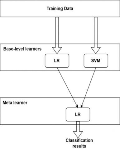
3.5 Ensemble learning based stacking model for FP grade
The term "ensemble learning methods" refers to different types of algorithms that aggregate the findings of more than one model. They are designed in order to improve the prediction outcomes based on the learning of more than one classifier. Bagging, boosting, and stacking are three approaches to the various classifier combination strategies that have been developed. An ensemble classifier has its own benefits and drawbacks. In this work, a novel ensemble stacking method for classifying the degrees of FP was developed. Figure 3 depicts the flowchart for the new ensemble stacking approach. There are two stages of learning involved in the classification process: the base level and the meta-level.
Figure 3. Flowchart for the new ensemble stacking approach
At the base level, two classifiers called SVM and LR are used. These classifiers are trained and tested simultaneously on the features that are derived from the fusion modalities independently. The RBF kernel is utilized for the SVM algorithm; this kernel will require two parameters, which are C and gamma. The grid-search method and five-fold cross-validation are used to discover the best values for the hyperparameters. At the meta-level, the FP grade is determined by combining two prediction results from the base level and providing those combined findings as input to a meta-level classifier (i.e., LR).
3.6 Performance metrics
The evaluation metrics utilized to determine the performance of the classifier are accuracy, precision, recall, and the F1-score. Following is an explanation of each of the metrics that were utilized for this investigation.
$Accuracy=\frac{TP+TN}{TP+TN+FP+FN}$ (10)
$Precision=\frac{TP}{TP+FP}$ (11)
$Recall=\frac{TP}{TP+FN}$ (12)
$F1=2*\frac{precision*recall}{precision*recall}$ (13)
where, TP is the true positive (i.e., FP samples), TN is the true negative (i.e., control group samples), FP is the false positive and FN is the false negative which are misclassified samples.
In this section, we examine the performance of the four machine learning models on our dataset. In this work, two novel models for FP detection and FP grade classification are introduced.
4.1 FP detection model performance
To find the best FP detection model, we performed different experiments in two ways: raw features and dimensionality reduction techniques (PCC, PCA, and PCC+PCA) using two kinds of feature vectors. First, individual feature vectors (LM, AU, EM), and second, fused features (LM+AU+EM). For both experiments, we employed four ML classifiers (i.e., LR, DT, NB, and SVM). Table 5 reports experimental results using individual feature sets of four classifiers with raw features and dimensionality reduction techniques. Similarly, Table 6 presents the experimental results using the fused features of four classifiers with raw feature dimensionality reduction techniques.
Figure 4 gives a visualization of performance metrics with different experiments. Figure 4a shows the bar chart of ML classifiers on raw data. Here, the ML models receive 522 features as input. On the raw data, the SVM classifier achieved the best accuracy of 80%, precision of 79.5%, recall of 85.4%, and F1 of 82.4%. Figure 4b depicts the bar chart of four ML model metrics on PCC data. Compared with raw features, PCC-extracted features perform well on all four ML classifiers. In this experiment, out of 522 features, 333 are found redundant; after removing these features from the raw data, the resultant features are 189. In order to determine the optimal model for the PCC data, these 189 features are fed into machine learning (ML) models. Among the four classifiers, LR and SVM, both algorithms are performing equally well, with 90.7% accuracy. Next, we compared the results of the classifiers using PCA data (see Figure 4c). In this experiment, all 522 features are transformed into reduced principal components (PCs). Here, we experimented with different component combinations (i.e., 30–40 PCs). Here, SVM produced the best performance values compared to SVM performance values on raw data with accuracy, precision, recall, and F1 values of 86.7%, 89.7%, and 87.5%, respectively. Compared with raw data features, reduced feature data (PCA) gives the best performance. When we compare PCA with PCC data, PCC features exhibit the best results. Due to this reason, we plan to apply PCA after reducing redundant features from the raw data (i.e., PCC+PCA). Figure 4d shows the performance metrics values of four ML classifiers on PCC+PCA data. The SVM algorithm outperforms others with the highest accuracy of 97.7% and precision, recall, and F1 of 98.1%. It is the highest among all the experiments performed—the next highest accuracy achieved by using LR with an accuracy of 94.7%.
Table 5. Performance of different ML classifiers on individual facial features
|
Individual Features |
ML Classifier |
Landmark (LM) |
Action Unit (AU) |
Eye Movement (EM) |
|||
|
No. of Features |
Accuracy (%) |
No. of Features |
Accuracy (%) |
No. of Features |
Accuracy (%) |
||
|
Raw features |
LR |
270 |
57.3 |
228 |
82.7 |
24 |
72 |
|
DT |
84 |
72 |
68 |
||||
|
NB |
62.3 |
80 |
64 |
||||
|
SVM |
68 |
85.3 |
73.3 |
||||
|
PCC |
LR |
44 |
80 |
135 |
90.7 |
24 |
77.3 |
|
DT |
78.7 |
80 |
73.3 |
||||
|
NB |
62.7 |
77.3 |
72 |
||||
|
SVM |
84 |
89.3 |
74.7 |
||||
|
PCA |
LR |
15-20 PCs |
84 |
35-40 PCs |
84 |
15-20 PCs |
74.7 |
|
DT |
78.7 |
72 |
66.7 |
||||
|
NB |
72 |
72 |
58.7 |
||||
|
SVM |
88 |
82.7 |
73.3 |
||||
|
PCC+PCA |
LR |
15-20 PCs |
86 |
35-40 PCs |
91.8 |
15-20 PCs |
79 |
|
DT |
80.6 |
82.3 |
76.8 |
||||
|
NB |
76.8 |
79.3 |
81.3 |
||||
|
SVM |
90.1 |
91 |
77.9 |
||||
Table 6. Performance of different ML classifiers on fused facial features
|
Individual Features |
ML Classifier |
Fused Features (LM+AU+EM) |
||||
|
No. of Features |
Accuracy (%) |
Precision (%) |
Recall (%) |
F1 (%) |
||
|
Raw features |
LR |
522 |
65.3 |
64.7 |
80.5 |
71.7 |
|
DT |
65.3 |
66.7 |
73.2 |
69.8 |
||
|
NB |
61.3 |
61.9 |
59.1 |
57.7 |
||
|
SVM |
80 |
79.5 |
85.4 |
82.4 |
||
|
PCC |
LR |
189 |
90.7 |
92.5 |
90.2 |
91.4 |
|
DT |
77.3 |
78.6 |
80.5 |
79.5 |
||
|
NB |
78.7 |
81 |
77.2 |
77.5 |
||
|
SVM |
90.7 |
90.5 |
92.7 |
91.6 |
||
|
PCA |
LR |
30-40 PCs |
84 |
89.2 |
80.5 |
84.6 |
|
DT |
68 |
73 |
65.9 |
69.2 |
||
|
NB |
70.7 |
70.4 |
70.4 |
70.4 |
||
|
SVM |
86.7 |
89.7 |
85.4 |
87.5 |
||
|
PCC+PCA |
LR |
30-40 PCs |
94.7 |
95.1 |
95.1 |
95.1 |
|
DT |
86.7 |
86 |
90.2 |
88.1 |
||
|
NB |
82.7 |
83.3 |
85.4 |
84.3 |
||
|
SVM |
97.7 |
98.1 |
98.1 |
98.1 |
||
Based on the above discussion, our findings are as follows: First, when compared with individual features, fused features performed more effectively. Second, the best dimensionality reduction technique for FP detection is the combined approach (principal component analysis with Pearson correlation coefficient, i.e., PCC+PCA).
(a)
(b)
(c)
(d)
Figure 4. Performance metrics of four different machine learning algorithms on different feature sets. a) All features, b) selected features after Pearson correlation, c) reduced features after PCA, d) PCC + PCA features
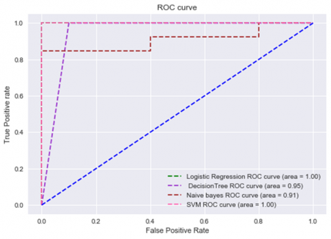
Figure 5. ROC curves of four ML classifiers on PCC+PCA data
The receiver operating characteristic curve (ROC curve) is a graph that displays how well a classification model performs across all classification thresholds. Figure 5 depicts the four ML classifiers ROC curves and the area under the curve values. These values are computed using accuracy, precision, recall, and the F1 score. Our observations from Figure 5 are that LR and SVM perform well with an AUC value of 100%, DT performed moderately with an AUC value of 95%, and NB gave poor performance with an AUC value of 91%.
Based on the above experimentation, we came to know that the SVM ML algorithm on fused features with PCC+PCA dimensionality reduction is the best model for predicting FP detection.
4.2 Ensemble learning based stacking model performance for FP grade
It is aimed at finding the grading of FP using fused features using the same approach experimented with in the previous section, i.e., PCC+PCA. It is noted that this approach performed better for FP detection but not for grading FP. The experimental results of four base classifiers are given in Table 7. From the table, it is found that these models performed moderately for FP grade classification.
The ensemble learning-based stacking approach aims to improve the performance of the FP grade classification. Using LR and SVM classifiers, an ensemble learning-based stacking approach was constructed. These classifiers were selected because they performed better when compared with DT and NB, as shown in Table 7.
Figure 6. Performance metrics of four single ML algorithms and proposed ensemble learning based stacking approach on PCC+PCA features
Table 7 also reports stacking method performance metrics. It is observed that the stacking method outperformed accuracy by 5.3%, precision by 0.5%, recall by 5.2%, and F1 score by 1.9% compared to LR. The reason for comparison with LR is that it performed better compared to other base classifiers in terms of accuracy. Figure 6 depicts a comparison of the performance metrics between the stacking approach and base classifiers for FP-grade classification.
4.3 Comparing the suggested model to latest studies
Rigorous comparative analysis is required to fully evaluate the novelty and effectiveness of the proposed method for FP detection and grade classification. We aim to benchmark our model against existing methods in the literature, considering a variety of methods, including landmark-based models, eye movement features, action unit features, and other state-of-the-art techniques. This comparative evaluation serves several purposes. First, we can quantitatively measure the performance of the proposed approach against established benchmarks and clearly demonstrate its superiority and competitive advantage. A comparison with the results obtained with existing methods then provides valuable insight into the strengths and weaknesses of different methods. This comparative framework also helps us understand the specific contributions and innovations that our model brings to the field of FP detection. Through this analysis, we not only establish the robustness of our proposed approach but also contribute to the broader knowledge base by highlighting progress and room for improvement in the field of FP assessment.
In this subsection, we compare the performance of the proposed two models with the latest studies. We validated our first model (i.e., FP detection) with the methodology used in the research [19]. The authors [19] used the Toronto Neuro Face dataset (TNF) [30] for FP detection. On the same dataset, we experimented with our FP detection technique (a binary classifier). Our method outperformed with an increased accuracy of 1.28%. Next, we compared the performance of our second model (i.e., FP grade classification) with the methodology used in the research [8] on FPara dataset. The FP grade classification method outperformed with an increased accuracy of 8.3%; comparison results are reported in Table 8.
Table 7. Performance of a single machine learning model compared to the suggested ensemble stacking method for grading FP
|
|
ML Classifier |
Accuracy (%) |
Precision (%) |
Recall (%) |
F1 (%) |
|
PCC+PCA |
LR |
82.9 |
82.8 |
82.3 |
87.3 |
|
DT |
78 |
79.3 |
86.5 |
83.6 |
|
|
NB |
73.2 |
71.3 |
69 |
69.6 |
|
|
SVM |
80.5 |
82.1 |
86.5 |
85.2 |
|
|
Stacking |
88.2 |
83.3 |
87.5 |
89.2 |
Table 8. Comparison of suggested models with latest studies
|
Latest Study |
Feature Category |
Classification Problem Type |
Database |
Strategy |
Accuracy |
|
[20] |
LM |
Binary |
Own database* |
SVM |
70% |
|
[19] |
LM |
Binary |
TNF |
MLP |
97.22% |
|
[11] |
EAR |
Multi class |
Own database* |
DT |
85.70% |
|
[8] |
LM |
Multi class |
FPara dataset* |
ALGRNet |
75.4% |
|
Our Method (FP detection) |
LM+AU+ EM |
Binary |
TNF |
SVM |
98.5% |
|
Our Method (FP grade) |
LM+AU+ EM |
Multi class |
FPara dataset* |
Ensemble stacking |
83.7% |
Note: LM: Landmarks, SVM: Support Vector Machine, EAR: Eye Aspect Ratio, MLP: Multi-Layer Perceptron, DT: Decision Tree, ALGRNet: Adaptive Local-Global Relational Network, AU: Action Units, EM: Eye Movement. * Not comparable; authors used their own dataset.
In this research, two novel models are proposed. The first model is for FP detection (i.e., a binary classifier) to identify whether the person has FP or is healthy. The second model is for FP grade prediction (i.e., normal, mild, moderate, or severe). To determine the best FP detection model, we conducted various experiments using four base classifiers with individual features (LM, AU, and EM) and fused features (LM+AU+EM) to identify the optimal feature set. Different dimensionality reduction techniques (PCC, PCA) were also applied. Among all the experiments, the SVM classifier achieved an accuracy of 97.7% on fused features with PCC+PCA dimensionality reduction. For FP grade classification, a novel ensemble learning-based stacking approach was developed based on LR and SVM algorithms. LR and SVM algorithms were used as base-level learners, and predictions of these models were given as input to the meta-learner (i.e., LR) in the next level. From the meta-learner, we can obtain the predicted labels for FP grade. This approach achieved an accuracy of 88.2%. The research findings could assist clinicians in identifying patients with FP early and continuously monitoring them. The proposed FP detection model can be applied to telemedicine to remotely monitor patients, enabling healthcare professionals to assess facial nerve function without a direct visit.
The proposed FP detection and grade classification models, like any models, exhibit potential limitations and are based on certain assumptions. Recognizing these aspects is crucial for a nuanced interpretation of results and guiding future improvements. Limitations include reliance on the diversity and representativeness of the training dataset, with potential compromises in generalization if it lacks variability in demographic factors, severity levels, or causes of FP. Interpersonal variability in facial expressions poses a challenge, particularly in populations with diverse ethnicities and age groups. The inherent difficulty in assigning precise grades due to the subjective nature of grading systems introduces ambiguity in predictions. Real-time applications may be constrained by processing speed and computational resources.
Some limitations of this work, due to the unavailability of FP public datasets, include considering only four severity levels. Furthermore, additional severity-level classes could be added to the database in future studies. In the future, we can address more diseases with this model, which we can find by using facial features.
[1] Goyal, D., Jerripothula, K.R., Mittal, A. (2020). Detection of gait abnormalities caused by neurological disorders. In 2020 IEEE 22nd International Workshop on Multimedia Signal Processing (MMSP), Tampere, Finland, pp. 1-6. https://doi.org/10.1109/MMSP48831.2020.9287163
[2] Gogu, S.R., Sathe, S.R. (2023). autoFPR: An efficient automatic approach for facial paralysis recognition using facial features. International Journal on Artificial Intelligence Tools, 32(02): 2340005. https://doi.org/10.1142/S0218213023400055
[3] Gautam, R., Sharma, M. (2020). Prevalence and diagnosis of neurological disorders using different deep learning techniques: A meta-analysis. Journal of Medical Systems, 44(2): 49. https://doi.org/10.1007/s10916-019-1519-7
[4] Raghavendra, U., Acharya, U.R., Adeli, H. (2020). Artificial intelligence techniques for automated diagnosis of neurological disorders. European Neurology, 82(1-3): 41-64. https://doi.org/10.1159/000504292
[5] Liu, Y., Xu, Z., Ding, L., Jia, J., Wu, X. (2021). Automatic assessment of facial paralysis based on facial landmarks. In 2021 IEEE 2nd International Conference on Pattern Recognition and Machine Learning (PRML), Chengdu, China, pp. 162-167. https://doi.org/10.1109/PRML52754.2021.9520746
[6] Baugh, R.F., Basura, G.J., Ishii, L.E., et al. (2013). Clinical practice guideline: Bell’s palsy. Otolaryngology–Head and Neck Surgery, 149(3_suppl): S1-S27. https://doi.org/10.1177/0194599813505967
[7] Ngo, T.H., Chen, Y.W., Matsushiro, N., Seo, M. (2016). Quantitative assessment of facial paralysis based on spatiotemporal features. IEICE Transactions on Information and Systems, 99(1): 187-196. https://doi.org/10.1587/transinf.2015EDP7082
[8] Ge, X., Jose, J. M., Wang, P., Iyer, A., Liu, X., Han, H. (2022). Automatic facial paralysis estimation with facial action units. arXiv preprint arXiv:2203.01800. https://arxiv.org/abs/2203.01800.
[9] Barrios Dell'Olio, G., Sra, M. (2021). Farapy: An augmented reality feedback system for facial paralysis using action unit intensity estimation. In The 34th Annual ACM Symposium on User Interface Software and Technology, pp. 1027-1038. https://doi.org/10.1145/3472749.3474803
[10] Ansari, S.A., Jerripothula, K.R., Nagpal, P., Mittal, A. (2022). Eye-focused Detection of Bell's Palsy in Videos. arXiv preprint arXiv:2201.11479. https://arxiv.org/abs/2201.11479.
[11] Feng, J., Guo, Z., Wang, J., Dan, G. (2020). Using eye aspect ratio to enhance fast and objective assessment of facial paralysis. Computational and Mathematical Methods in Medicine, 2020: 1038906. https://doi.org/10.1155/2020/1038906
[12] Wang, T., Zhang, S., Liu, L.A., Wu, G., Dong, J. (2019). Automatic facial paralysis evaluation augmented by a cascaded encoder network structure. IEEE Access, 7: 135621-135631. https://doi.org/10.1109/ACCESS.2019.2942143
[13] Zhuang, Y., McDonald, M.M., Aldridge, C.M., Hassan, M.A., Uribe, O., Arteaga, D., Southerland, A.M., Rohde, G.K. (2021). Video-based facial weakness analysis. IEEE Transactions on Biomedical Engineering, 68(9): 2698-2705. https://doi.org/10.1109/TBME.2021.3049739
[14] Hsu, G.S.J., Kang, J.H., Huang, W.F. (2018). Deep hierarchical network with line segment learning for quantitative analysis of facial palsy. IEEE Access, 7: 4833-4842. https://doi.org/10.1109/ACCESS.2018.2884969
[15] Chrysos, G.G., Antonakos, E., Zafeiriou, S., Snape, P. (2015). Offline deformable face tracking in arbitrary videos. In Proceedings of the IEEE International Conference on Computer Vision Workshops, Santiago, Chile, pp. 954-962. https://doi.org/10.1109/ICCVW.2015.126
[16] Shen, J., Zafeiriou, S., Chrysos, G.G., Kossaifi, J., Tzimiropoulos, G., Pantic, M. (2015). The first facial landmark tracking in-the-wild challenge: Benchmark and results. In Proceedings of the IEEE International Conference on Computer Vision Workshops, Santiago, Chile, pp. 50-58. https://doi.org/10.1109/ICCVW.2015.132
[17] Tzimiropoulos, G. (2015). Project-out cascaded regression with an application to face alignment. In Proceedings of the IEEE Conference on Computer Vision and Pattern Recognition, Boston, MA, USA, pp. 3659-3667. https://doi.org/10.1109/CVPR.2015.7298989
[18] Baltrušaitis, T., Robinson, P., Morency, L.P. (2016). Openface: An open source facial behavior analysis toolkit. In 2016 IEEE Winter Conference on Applications of Computer Vision (WACV), Xi'an, China, pp. 1-10. https://doi.org/10.1109/FG.2018.00019
[19] Parra-Dominguez, G.S., Sanchez-Yanez, R.E., Garcia-Capulin, C.H. (2021). Facial paralysis detection on images using key point analysis. Applied Sciences, 11(5): 2435. https://doi.org/10.3390/app11052435
[20] Afifi, N., Diederich, J., Shanableh, T. (2006). Computational methods for the detection of facial palsy. Journal of Telemedicine and Telecare, 12(3_suppl): 3-7. https://doi.org/10.1258/135763306779380129
[21] Barbosa, J., Seo, W.K., Kang, J. (2019). paraFaceTest: an ensemble of regression tree-based facial features extraction for efficient facial paralysis classification. BMC Medical Imaging, 19: 1-14. https://doi.org/10.1186/s12880-019-0330-8
[22] Sajid, M., Shafique, T., Baig, M.J.A., Riaz, I., Amin, S., Manzoor, S. (2018). Automatic grading of palsy using asymmetrical facial features: A study complemented by new solutions. Symmetry, 10(7): 242. https://doi.org/10.3390/sym10070242
[23] Hsu, G.S.J., Huang, W.F., Kang, J.H. (2018). Hierarchical network for facial palsy detection. In CVPR Workshops, pp. 580-586. https://doi.org/10.1109/CVPRW.2018.00100
[24] Storey, G., Jiang, R., Keogh, S., Bouridane, A., Li, C.T. (2019). 3DPalsyNet: A facial palsy grading and motion recognition framework using fully 3D convolutional neural networks. IEEE Access, 7: 121655-121664. https://doi.org/10.1109/ACCESS.2019.2937285
[25] Xu, P., Xie, F., Su, T., Wan, Z., Zhou, Z., Xin, X., Guan, Z. (2020). Automatic evaluation of facial nerve paralysis by dual-path LSTM with deep differentiated network. Neurocomputing, 388: 70-77. https://doi.org/10.1016/j.neucom.2020.01.014
[26] Zhang, K., Zhang, Z., Li, Z., Qiao, Y. (2016). Joint face detection and alignment using multitask cascaded convolutional networks. IEEE Signal Processing Letters, 23(10): 1499-1503. https://doi.org/10.1109/LSP.2016.2603342
[27] Zhang, L., Tjondronegoro, D. (2011). Facial expression recognition using facial movement features. IEEE Transactions on Affective Computing, 2(4): 219-229. https://doi.org/10.1109/T-AFFC.2011.13
[28] Braathen, B., Bartlett, M.S., Littlewort, G., Movellan, J.R. (2001). First steps towards automatic recognition of spontaneous facial action units. In Proceedings of the 2001 Workshop on Perceptive User Interfaces, pp. 1-5. https://doi.org/10.1145/971478.971515
[29] Pearson, K. (1894). Contributions to the Mathematical Theory of Evolution. Royal Society.
[30] Bandini, A., Rezaei, S., Guarín, D.L., Kulkarni, M., Lim, D., Boulos, M.I., Zinman, L., Yunusova, Y., Taati, B. (2020). A new dataset for facial motion analysis in individuals with neurological disorders. IEEE Journal of Biomedical and Health Informatics, 25(4): 1111-1119. https://doi.org/10.1109/JBHI.2020.3019242