Meghraoui Mohamed Hamza*![]() | Benaired Noreddine
| Benaired Noreddine![]() | Benselama Zoubir Abdeslem
| Benselama Zoubir Abdeslem![]() | Yssaad Benyssaad
| Yssaad Benyssaad![]() | Benselama Sarah Ilham
| Benselama Sarah Ilham![]()
© 2024 The authors. This article is published by IIETA and is licensed under the CC BY 4.0 license (http://creativecommons.org/licenses/by/4.0/).
OPEN ACCESS
In the realm of cardiovascular disease (CVD) diagnostics, the morphological changes in arterial blood pressure (ABP) attributable to various pathologies have long been recognized. This study explores the innovative intersection of photoplethysmography (PPG) signals and machine learning (ML) techniques, focusing on the classification of abnormal arterial pulse (AAP) patterns, a domain hitherto not extensively researched. The challenges of this endeavor, primarily the scarcity of clinically labeled AAP waveform datasets, are acknowledged. This scarcity stems from the difficulty in sourcing volunteers exhibiting diverse disease-related AAPs and the inherent risks associated with ABP measurement procedures. Furthermore, current guidelines do not sufficiently characterize AAP traits, limiting the application of PPG and ML in detecting ABP-related anomalies predominantly to hypertension and hypotension cases. Addressing these gaps, the present study introduces a PPG-based classification system employing k-nearest neighbors (KNN) and bagged trees (BT) algorithms. These were selected for their proficiency in modeling complex, nonlinear relationships while maintaining lower complexity levels compared to alternatives like Deep Neural Networks (DNN) or Support Vector Machines (SVM). Additionally, novel detectors have been developed for identifying key pulse wave features such as troughs and dicrotic notches, crucial for AAP pattern recognition and PPG feature extraction. The methodology encompasses a modeling process that references pathological cases known to manifest specific AAP patterns. An extensive evaluation involving 1,120 PPG and ABP signals yielded impressive accuracies of 90.9% and 91% for KNN and BT algorithms, respectively. Across 11 distinct classes, both algorithms exhibited robust performance, underscoring their potential as effective AAP detectors. These results signify an advancement over existing classifiers, particularly in generating multiple CVD-related classes with reduced complexity at both modular and instance levels. The system's capability to associate AAPs with CVDs positions it as a promising, non-invasive, and cost-effective tool for diverse applications including doctor-assisted diagnosis, remote post-surgery monitoring, nursing alerts, and personalized health management. This approach not only meets emerging healthcare needs but also mitigates the risks associated with current invasive diagnostic practices.
abnormal arterial pulse (AAP), arterial blood pressure (ABP), classification, machine learning (ML), modeling, photoplethysmography (PPG)
CVDs remain the leading cause of fatalities globally [1], and their burden is projected to grow if left unaddressed. CVDs often present with mild, progressively worsening symptoms [2] and sometimes remain asymptomatic until sudden cardiac death [3]. Early and accurate detection is critical to encourage lifestyle changes and medical intervention if needed [4]. Clinically, CVD diagnosis faces challenges as symptoms are heterogeneous and non-specific [5], resulting in delays and poorer prognoses [5, 6]. Conventional diagnostic criteria have limitations in sensitivity and specificity for CVDs and may produce false positives [5]. Healthcare must leverage automated, intelligent systems to address CVD management concerns. PPG offers a convenient, noninvasive way to measure pulsatile blood volume changes, revealing cardiovascular insights [7]. PPG uses light-based sensing to capture signals from flexible locations like the wrist, finger, or earlobe [8]. With recent advances in ML, PPG has emerged as a favorable biosensing option for early CVD prediction [9].
Existing PPG-based CVD prediction systems tend to be more pathologically specific. Putra et al. [10] explored feature selection methods to optimize KNN performance for coronary heart disease (CHD) classification. Hackstein et al. [11] used naive Bayes (NB) and KNN classifiers with feature selection to predict aortic aneurysms. Hosseini et al. [12] used time-domain PPG features to identify the risk of coronary artery disease (CAD) using a KNN classifier. De Moraes et al. [13] investigated four classifiers to identify cardiopathies using temporal features. Other researchers leveraged PPG signals for CVD-risk classification [14, 15]. Prabhakar et al. [14] used artificial neural networks (ANN) and logistic regression (LR) to classify CVD risk from dimensionally optimized PPG data. Palanisamy and Rajaguru [9] used 12 classifiers to identify CVD-risk from dimensionally reduced PPG signals.
While the aforementioned works showed promising results, enhancing healthcare infrastructure goes beyond classifiers performances. For these systems to meaningfully support medical services, two sets of questions need to be asked:
(1) How might these systems potentially assist physicians in screening and risk profiling procedures? What limitations may exist?
(2) Can physicians make clinical decisions for patients without awareness of the underlying reasoning [16]? How can trust be fostered?
The former questions address the system’s predictive capacity. Systems focusing on single diseases in studies [10-13] may confirm diagnoses or refine risk profiles but have limited utility for initial broad screening. A more versatile classifier capable of multiple outputs could provide a broader perspective and guidance on potential CVDs. On the other hand, systems targeting general cardiovascular risk in studies [9, 14, 15] provide limited etiological insights for clinical decision-making. These approaches rely on observable respiratory events like rebreathing, heart variability, and apnea [17]. Such diverse, non-specific symptoms can complicate the prognosis and delay diagnosis [6].
The latter questions address clinical decision-making transparency. Evidence-based medicine relies on understanding pathophysiology rather than direct outputs alone [16]. Regardless of whether a system predicts specific CVDs or general risk levels, a lack of insight into its underlying logic limits its real-world applicability. Gaining acceptance within the medical community requires providing more targeted insights into probable disease factors. However, existing research may overemphasize predictive performance at the expense of applicability and transparency. For instance, extracting features through complex optimization algorithms is clinically irrelevant; what is needed are physiologically meaningful features, not perfect dimensionally reduced features [9, 14].
Ultimately, an ideal system would support nuanced risk profiling and initial screening through multiple, evidence-based outputs. An underexplored solution that may address these needs is targeting ABP morphologies. The pathophysiology of CVD is known to impact the ABP waveform, resulting in AAP patterns related to various CVDs [18-20]. For instance, the bisferiens pulse is seen in aortic regurgitation (AR), hypertrophic obstructive cardiomyopathy (HOCM), or mixed valvular heart diseases (VHDs) [19]. Patterns like tardus, parvus et tardus, and anacrotic indicate severe aortic stenosis (AS). The dicrotic pulse is associated with low cardiac output conditions [21, 22]. Deep pulses may signify low vascular resistance or sepsis [23, 24]. Bounding pulses involve arteriovenous fistulas, or AR, among others [19]. Water hammer pulses are typical of severe AR [25]. Importantly, clinical evidence could identify these abnormalities. Unfortunately, the use of PPG and ML in classifying ABP-related abnormalities is limited to hypertension [26] or hypotension [27].
One limitation is the lack of clinical datasets containing labeled AAP waveforms, likely due to the risks involved with measuring ABP [28]. Developing such datasets poses challenges, as it requires finding and monitoring volunteers exhibiting various disease-related AAPs. However, the MIMIC-III database offers a potential solution as it contains thousands of synchronous ABP-PPG recordings spanning hours from intensive care patients [29]. Interestingly, it incorporates diverse ABP morphologies, a valuable opportunity to address the lack of labeled AAP data. Nevertheless, challenges persist since no standards exist for identifying AAPs.
The goal of this study was to create a PPG-based system that could sort already-known AAPs into groups, including bisferiens, anacrotic, tardus, parvus et tardus, dicrotic, deep, bounding, and water hammer. Two ML techniques were adopted, including KNN and BT classifiers. This research followed three main steps:
(1) ABP and PPG recordings were continuously collected from two MIMIC databases to ensure AAP diversity. Signals underwent preprocessing to eliminate noise and baseline drift. Custom detectors were developed for pulse feature detection. Troughs were located using third-derivative analysis to partition signals into individual pulses. Dicrotic notches were detected via a multi-objective optimizer conducting an iterative search within a predefined parameter space.
(2) Clinical literature was then referred to as model AAPs. Amplitude analysis identified patterns in widened (bounding) or narrowed (parvus et tardus) pulse pressure. Contour examination featured abnormalities such as double peaks (bisferiens, anacrotic), enlarged dicrotic waves (dicrotic pulse), or sharp waves (water hammer). Temporal analysis involved detecting delayed (tardus, parvus et tardus, slow-bounding) or shortened (water hammer) time to peak pressure. PPG pulse morphology was then analyzed using temporal and statistical metrics to extract features. Metrics like kurtosis, mean, slope, and duration of waves tied to cardiac events were quantified.
(3) KNN and BT classifiers were chosen to balance modeling simplicity while imposing minimal assumptions on the nonlinear data. KNN utilizes proximity-based labeling, assuming similar instances are nearby [30]. BT averages predictions from decision trees (DTs), leveraging trees' simplicity while reducing overfitting [31, 32]. A comparative evaluation of several ML classifiers on a subset of the data validated their effectiveness. Hyperparameters were then optimized to maximize accuracy. The tuned KNN and BT models were then trained on the full dataset and cross-validated via k-folding.
This study addresses current limitations by enabling the non-invasive identification of various pressure-related abnormalities from PPG signals alone. Whereas previous work predominantly estimated ABP waveforms using ML techniques [33], this research introduces the detection of irregularities that may manifest within these waveforms. While PPG signals have been utilized to predict various cardiovascular, sleep, mental health, and metabolic conditions [34], their use in predicting ABP-related abnormalities is limited to hypertension and hypotension [26, 27]. Overall, the developed methodology presents a novel means of characterizing pathological hemodynamic phenotypes for improved CVD assessment.
The paper is organized as follows: Section II introduces the proposed methodology, covering data acquisition, pulse wave feature detection, AAP modeling, feature engineering, and the proposed ML experiment. Section III presents the experimental results, provides further insights into the ML modeling process, and discusses the results. Comparisons are drawn between the current approach and prior related methods. Clinical implications are also explored, including potential medical contributions, system integration opportunities, and challenges. Finally, Section IV concludes the paper by summarizing the main contributions, limitations, and outlining potential directions for future work.
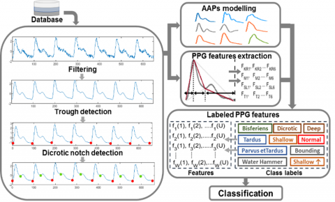
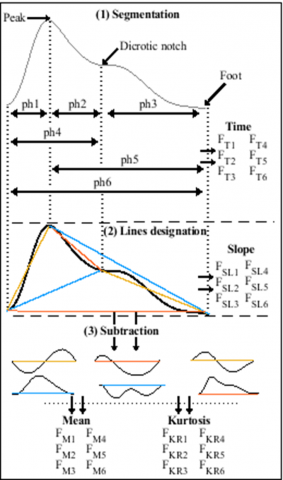
This section outlines our proposed methodology for classifying AAPs based on the steps illustrated in Figure 1.
Figure 1. Methodology steps
2.1 Data acquisition
In this study, we obtained our dataset from two publicly accessible databases, namely MIMIC and MIMIC III (Multiparameter Intelligent Monitoring in Intensive Care) [29, 35]. These databases provide a wide range of biomedical signals, particularly ABP and PPG signals, which were recorded simultaneously from patients in the intensive care unit (ICU). ABP signals were invasively measured through a catheter in the radial artery, while PPG signals were non-invasively captured using a fingertip sensor. Both signals have a sampling frequency (Fs) of 125 Hz.
2.2 Data selection
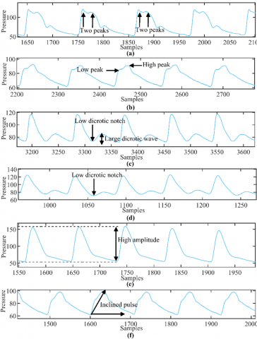
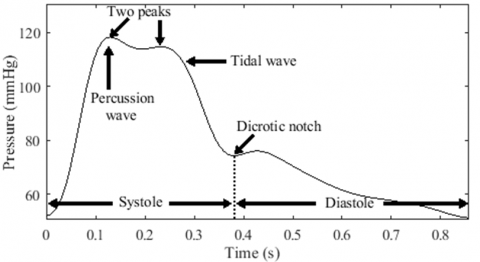
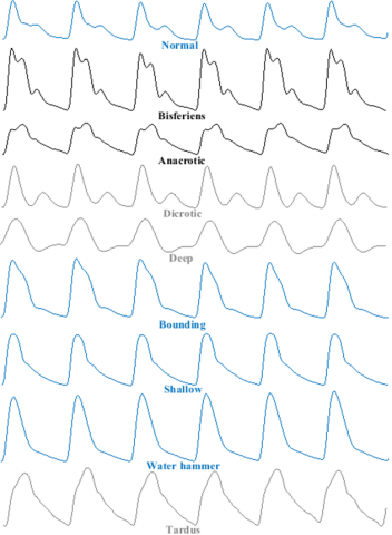
To ensure diversity of AAPs and good signal quality, a manual selection process was conducted for ABP and PPG records from the MIMIC databases. While records were being kept, each ABP was looked at visually for possible AAP patterns, such as bisferiens, anacrotic, dicrotic, deep, bounding, and tardus pulses (Figure 2). In particular, two systolic peaks helped us tell the difference between bisferiens and anacrotic pulses. Anacrotic pulses were set apart by a lower first peak (Figure 2 (a), (b)). Dicrotic and deep pulses showed abnormally low dicrotic notches (Figure 2 (c), (d)), with dicrotic pulses having larger dicrotic waves (Figure 2(d)). Bounding pulses had abnormally high amplitudes (Figure 2(e)). Tardus pulses appeared inclined to the right due to a delayed peak time (Figure 2 (f)).
The process continued until a reasonable number of AAP examples were observed. Some records containing AAPs were excluded due to poor PPG signal quality, which is highly susceptible to motion artifacts [36]. The selection process was the most challenging and time-consuming part of the study. However, over a thousand records were collected, each lasting one minute and containing a diverse range of AAPs.
Figure 2. Abnormal patterns in ABP signals
2.3 Signal preprocessing
There are a lot of bad effects on the signals that come from the MIMIC and MIMIC III databases. These include high-frequency noise and baseline drift in PPG signals, as well as noisy changes in ABP signals. To address these effects, we employ two filtering techniques. First, we use a fourth-order Butterworth filter with a bandpass range of 0.5 Hz to 8 Hz to get rid of baseline drift and high-frequency noise in PPG signals [33]. Secondly, we used a moving average filter to remove noisy fluctuations from ABP signals.
2.4 Segmentation
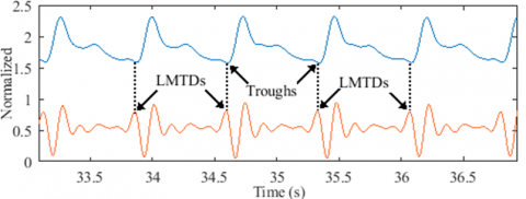
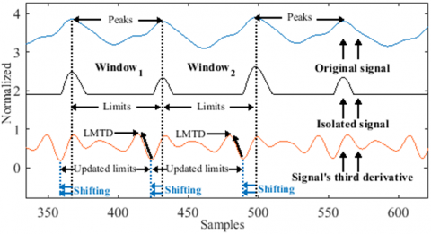
To extract pulses from the records, we performed a segmentation process based on the signal’s third derivative. Our research showed that every signal trough is closely linked to a local maximum in the signal's third derivative (Figure 3(a)). We call this the Local Maximum Third Derivative (LMTD). Interestingly, these LMTDs can still be seen in records where the troughs aren't (Figure 3(b)), which suggests that they could be used to get a rough idea of suppressed troughs.
As depicted in Figure 3, to locate an LMTD, we must first detect the last local minimum that precedes the signal’s peak (in green). As a result, three key points must be located to detect the trough: the peak, the last minimum preceding it, and the LMTD. The following steps explain in detail the segmentation procedure.
(a) Detectable troughs from an ABP record
(b) Suppressed troughs from a PPG record
Figure 3. LMTD locations
2.4.1 Normalization
To ensure that our signal is on a consistent scale, we normalize it using the z-score method. This involves centering and scaling the signal by its mean (μ) and standard deviation (δ), respectively. The following vectors represent the original signal retrieved from the dataset (Eq. (1)) and the normalized signal (Eq. (2)).
$X=\left\{x_1, x_2, x_n, \ldots \ldots x_N\right\}$ (1)
$X_{\text {norm }}=\left\{\frac{x_1-\mu}{\delta}, \frac{x_2-\mu}{\delta}, \frac{x_n-\mu}{\delta}, \ldots \ldots \frac{x_N-\mu}{\delta}\right\}$ (2)
where, x represents a single data point in the signal, n is the sample index and N is the length of the signal.
2.4.2 Peak detection
To locate the peaks of the signal, a threshold is initially established to isolate the prominent waves from the rest of the normalized signal, as indicated in Eq. (3). This method, known as clipping, is commonly employed by researchers for peak detection [37].
$T H=\frac{1}{N} \sum_{n=1}^N\left|X_{\text {norm }}\right|$ (3)
Next, we eliminate any part of the signal that falls below the threshold, as explained in Eq. (4).
$\begin{cases}S=X_{\text {norm }} & \text { if } X_{\text {norm }}>T H \\ S=T H & \text { otherwise }\end{cases}$ (4)
where, S represents the isolated signal.
Finally, we compare each sample to the threshold to identify the peak values. To prevent the identification of consecutive peaks within the same pulse, we set a minimum distance of 40 samples between any two identified peaks. By enforcing this condition, we can ensure that each peak corresponds to a distinct pulse within the signal.
2.4.3 LMTD detection
To detect the LMTDs, we first divide the signal’s third derivative into discrete windows (Eq. (5)). The limits of each window are set to the peak values of the original signal.
$X_{\text {norm }}^{\prime \prime \prime}=\left\{d_1, d_2, d_n, \ldots d_l, \ldots \ldots d_L\right\}$ (5)
where, $X_{\text {norm }}^{\prime \prime \prime}$ represents the normalized signal's third derivative, with each sample value denoted as $d$, the window's limit as $l$, and the last limit as $L$.
Next, we locate the local minima that precede the windows’ limits. We then update these limits by shifting them backward until they reach the local minima values, this results in a new set of limits as denoted in Eq. (6).
$X_{\text {norm }}^{\prime \prime \prime}=\left\{d_1, d_2, d_n, \ldots d_{l u}, \ldots \ldots d_{L u}\right\}$ (6)
where, the updated limit is designated as lu, and the final updated limit as Lu.
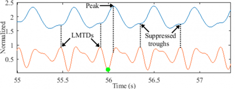
Finally, we identify the LMTDs as the local maxima preceding the updated limits. The process for detecting LMTDs is further illustrated in Figure 4.
Figure 4. LMTDs detection
To approximate the index values of the suppressed troughs, we examined the marginal distance between LMTDs and detectable troughs. Analysis of the signals revealed mean distances (MDs) and standard deviation distances (STDs) of 2.6±1.1 and 1.22±0.95 for ABP and PPG signals, respectively. As a result, the formula for approximating the suppressed troughs is defined as:
$t r_{\text {sup }}=L M T D_{i d x}+M D$ (7)
where, trsup denotes a suppressed trough, LMTDidx represents the LMTD index, and MD represents the mean distances.
2.5 Dicrotic notch detection
A dicrotic notch is typically identified by locating the local minimum at the end of the systolic phase. However, in the case of a suppressed dicrotic notch, a slight inflection point replaces the local minimum, making it difficult to detect using conventional methods. Therefore, we present a novel approach for detecting suppressed dicrotic notches using a multi-objective optimization technique.
2.5.1 Measurements
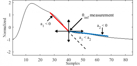
We introduce a tool that measures the angles of inflection points using two intersecting lines, as shown in Figure 5. Conventionally, the angle between two intersecting lines is calculated as follows:
$\theta=\tan ^{-1}\left(\frac{a_2-a_1}{1+a_1 a_2}\right)$ (8)
where, a1 and a2 are the slopes of the first and second lines, respectively.
However, this method is only valid when the signal axes are equally calibrated. Instead, we suggest estimating the inflection point measurements using a modified formula that considers the degree of deviation of one line relative to the other, as presented in Figure 5. Additionally, we impose constraints on the slopes of the intersected lines to ensure the exclusive measurement of the inflection points, as denoted in Eq. (9).
$\theta_{\text {inf }}=\frac{a_2-a_1}{a_1}$, such that $\left\{\begin{array}{c}a_1, a_2<0 \\ a_1<a_2\end{array}\right.$ (9)
where, θinf represents the degree of deviation of the second line compared to the first line, while inf is the inflection point index.
Figure 5. Measurement technique
2.5.2 Search space
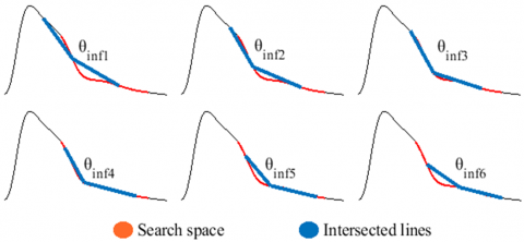
The search process involves obtaining a set of θinf measurements within a predetermined search space, which is delineated as a segment of the pulse wave extending between the peak and the trough (Figure 6). The pulse wave can be represented as a sequence of values, denoted as:
$P W=\left\{x_{t r}, x_{t r+1}, x_{t r+n}, \ldots x_{p e}, \ldots x_{t r+k}\right\}$ (10)
where, tr and pe respectively represent the pulse’s trough and peak indexes, while k indicates the pulse’s length.
The search space is then identified as a subset of PW, denoted as:
$S P=\left\{x_{\alpha_1}, \ldots \ldots x_{\alpha_2}\right\}$ (11)
where, α1 and α2 represent the indexes that mark the boundaries of the search space and are given by α1≈pe+0.55k and α2≈pe+0.15k.
Figure 6. Random θinf measurements in the search space
2.5.3 Search technique
The θinf measurements are taken by sliding the intersected lines along the entire search space while respecting the established constraints, as illustrated in Figure 6.
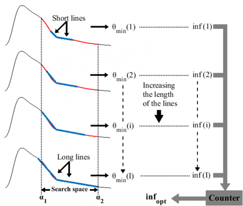
A suppressed dicrotic notch is indicative of an inflection point at the minimum-measurement θinf in the search space, denoted as θmin. However, a single search to obtain θmin may yield inaccurate measurements, leading to false positive results. As a result, we implement a search process involving multiple iterations (i) to identify the optimal solution (infopt). Within each iteration, measurements are taken using intersected lines of increasing lengths, resulting in varying slopes. In a given iteration, the slope of each line is defined as:
$\begin{gathered}a_{i, j}=\frac{f\left(c_{\text {end }}\right)-f\left(c_{\text {in }}\right)}{c_{\text {end }}-c_{\text {in }}} \\ \text { with }\left\{\begin{array}{l}c_{\text {in }}=\inf -i, c_{\text {end }}=\inf \text { when } j=1 \\ c_{\text {in }}=\inf , c_{\text {end }}=\inf +i \text { when } j=2\end{array}\right.\end{gathered}$ (12)
where, cin and cend represent the initial and the last sample index of a line, respectively, while f(cin) and f(cend) are their expected values. The length of the lines increases by i=1 during each iteration, until it reaches a maximum iteration of I≈0.15k.
Each of the resulting θmin(i) corresponds to a specific inf in the search space. Therefore, we determine infopt by considering all the θmin(i) measurements and their respective inf(i) obtained during the search process. We present the search process results φr for a particular pulse r as:
$\varphi_r=\left\{\begin{array}{c|c}\theta_{\min }(1) & \inf (1) \\ \theta_{\min }(2) & \inf (2) \\ \theta_{\min }(i) & \inf (i) \\ \vdots & \vdots \\ \theta_{\min }(I) & \inf (I)\end{array}\right\}$ (13)
The θmin measurements that were taken from similar indexes are counted to identify the most present inf in φr. As a result, the most prevalent inf(i) in φr is identified as infopt. The search process is further explained in Figure 7.
Figure 7. Search process
2.5.4 Evaluation process
To evaluate the efficacy of the optimization algorithm, we employ the standard deviation (SD) as a metric to ensure that the dicrotic notches are accurately located. Typically, the distance between a peak and its corresponding dicrotic notch is nearly constant across all pulses in a signal. Thus, the SD captures the variation between the optimal solutions infopt and the peaks throughout the entire signal Xnorm. The SD can be defined using the following equation:
$S D=\frac{\sum_{r=1}^R\left(i n f_{\text {opt }}(r)-p e(r)-\sigma\right)^2}{R}$ (14)
where, σ represents the mean distance between the peak and the optimal inflection point, while r denotes the index of each pulse and R represents the total number of pulses in the signal.
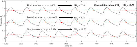
To further minimize the SD index, the search process is regenerated by gradually narrowing the search space (specifically α2) through three iterations until improved results are obtained, as depicted in Figure 8. If no improvement is observed, we select the search with the lowest SD value as the final result. Nevertheless, our analysis indicates that a marginal improvement of less than 1.38 is considered an instance of over-minimization. To address this, we have set a threshold to control the SD minimization process, requiring the SD index to improve by a value equal to or greater than 1.38.
To evaluate the efficacy of the proposed optimizer, Figure 8 presents a segment of a disrupted ABP signal. This particular signal was intentionally selected for its instability and association with various fluctuations, with the aim of testing whether any false positive dicrotic notches are detected.
Overall, our proposed algorithm incorporates three objective functions in an iterative manner. Firstly, we minimized θinf to obtain the minimum inflection point measurement (θmin). Secondly, we maximized φr to identify the optimal inflection point index (infopt). Finally, we minimized the SD index to improve the overall optimization process. Algorithm 1 displays a step-by-step pseudocode for the detection of the dicrotic notches within a signal.
Figure 8. A segment from an ABP signal during evaluation process
|
Algorithm 1: Dicrotic notches detector |
||||||||||
|
INPUT: |
Xnorm, Tr, Pe |
. 1-min ABP-PPG Signal, Troughs Vector, Peaks Vector |
||||||||
|
OUTPUT: |
dicroticnotch |
. Dicrotic Notches Vector |
||||||||
|
1 |
$y \leftarrow 0.55$ |
. y is the search space’s right boundary that needs decreasing during the evaluation process |
||||||||
|
2 |
for $n=1$ to 3 do |
. Evaluation process (overall optimization loop) |
||||||||
|
3 |
if $n==2$ than |
|
||||||||
|
4 |
|
$y \leftarrow 0.3$ |
. Narrowing the search space by decreasing y |
|||||||
|
5 |
elseif $n==3$ than |
|
||||||||
|
6 |
|
$y \leftarrow 0.2$ |
. Narrowing the search space by decreasing y |
|||||||
|
7 |
end if |
|
||||||||
|
8 |
function find_optimal_inf $\left(X_{\text {norm}}, T r, P e, y\right)$ |
. Search process function |
||||||||
|
9 |
|
Num$_{T r} \leftarrow$ length (Tr) |
. Number of troughs in a 1-min signal |
|||||||
|
10 |
|
for $r=1$ to $\quad\left(\mathrm{Num}_{T r}-1\right)$ do |
. A loop searching for infr of a given r pulse |
|||||||
|
11 |
|
|
$P W \leftarrow X_{\text {norm}}(\operatorname{Tr}(r): \operatorname{Tr}(r+1))$ |
. Pulse initialisation |
||||||
|
12 |
|
|
$k \leftarrow$ length $(P W)$ |
. The pulse’s length |
||||||
|
13 |
|
|
$\alpha_1 \leftarrow P e(r)+0.15 k$ |
. Left boundary of the search space |
||||||
|
14 |
|
|
$\alpha_2 \leftarrow P e(r)+y k$ |
. Right boundary of the search space |
||||||
|
15 |
|
|
$S P \leftarrow X_{\text {norm}}\left(\alpha_1: \alpha_2\right)$ |
. Search space indexes initialisation |
||||||
|
16 |
|
|
$f \leftarrow P W(S P)$ |
. Search space values initialisation |
||||||
|
17 |
|
|
$\mathrm{Num}_{\text {inf}} \leftarrow$ length $(S P)$ |
. Number of possible inflection points |
||||||
|
18 |
|
|
line $_{\text {lnit}} \leftarrow 3$ |
. Initial length value of the lines |
||||||
|
19 |
|
|
$I \leftarrow 0.15 k$ |
. Maximum length value |
||||||
|
20 |
|
|
for $i=$ line $_{\text {init}}$ to $I$ do |
. A loop for increasing the lines’ lengths starting from: lineinit=3 |
||||||
|
21 |
|
|
|
$m \leftarrow 1$ |
|
|||||
|
22 |
|
|
|
for $i n f_{\text {pos}}=1$ to $\left(\right.$ Num $\left._{\text {inf }}-1\right)$ do |
. Search process loop, infpos denotes a possible inf in the search space SP |
|||||
|
23 |
|
|
|
|
$a_1 \leftarrow\left(f\left(i n f_{p o s}\right)-f\left(i n f_{p o s}-i\right)\right) /\left(i n f_{p o s}-\left(i n f_{p o s}-i\right)\right)$ |
. Computing the value of the left slop |
||||
|
24 |
|
|
|
|
$a_2 \leftarrow\left(f\left(i n f_{p o s}+i\right)-f\left(i n f_{p o s}\right)\right) /\left(\left(i n f_{p o s}+i\right)-i n f_{p o s}\right)$ |
. Computing the value of the right slop |
||||
|
25 |
|
|
|
|
if $a_1, a_2<0$ and $a_1<a_2$ than |
. Constraints to ensure the exclusive measurement of inf |
||||
|
26 |
|
|
|
|
|
$\theta_{\text {inf }} \leftarrow\left(a_2-a_1\right) / a_1$ |
. Inflection point measurement |
|||
|
27 |
|
|
|
|
|
$\theta_{\text {store }}(m) \leftarrow \theta_{\text {inf }}$ |
. Storing the $\theta_{inf}$ measurements in the vector $\theta_{inf}$ |
|||
|
28 |
|
|
|
|
|
$\inf f_{\text {store }}(m) \leftarrow \inf f_{\text {pos }}$ |
. Storing the inf indexes in the vector infstore |
|||
|
29 |
|
|
|
|
|
$m \leftarrow m+1$ |
|
|||
|
30 |
|
|
|
|
end if |
|
||||
|
31 |
|
|
|
end for |
|
|||||
|
32 |
|
|
|
$\left\{\theta_{\text {min }}, \theta_{\text {min_ }}\right.$ index $\} \leftarrow \boldsymbol{\operatorname { m i n }}\left(\theta_{\text {store }}\right)$ |
. Extracting the index of the minimum $\theta_{inf}$ within the storage vector |
|||||
|
33 |
|
|
|
$\inf (i) \leftarrow$ inf$_{\text {store }}\left(\theta_{\text {min_}}\right.$ index $)$ |
. Matching the index with original infection point |
|||||
|
34 |
|
|
end for |
|
||||||
|
35 |
|
|
counter $\leftarrow$ count $(\varphi(r))$ |
. Counting similar inf(i) indexes |
||||||
|
36 |
|
|
$\inf _{\text {opt }}(r) \leftarrow $ max (counter) |
. The most prevalent inf(i) have the most counts |
||||||
|
37 |
|
|
dist_peak_to_inf $(r) \leftarrow i n f_{o p t}(r)-P e(r)$ |
. Distances between peaks and estimated $inf_{opt}$ |
||||||
|
38 |
|
end for |
|
|||||||
|
39 |
end function |
|
||||||||
|
40 |
signal$_{inf_{opt}}(n) \leftarrow inf_{opt}$ |
. The vector $signal_{inf_{opt}}$ represent the inf $inf_{opt}$ of the entire input signal $X_{norm}$ |
||||||||
|
41 |
dicrotic$_{notch } \leftarrow$ signal$_{inf_{opt}}(1)$ |
. Initialisation of the output vector |
||||||||
|
42 |
SD $\leftarrow$ std (dist_peak_to_inf) |
. Evaluation metric that measures the detection precision before re-looping the process |
||||||||
|
43 |
if $n==2$ and $S D(n)<S D(n-1)$ and $S D(n)>1.38$ than |
|
||||||||
|
44 |
|
dicrotic$_{notch} \leftarrow$ signal$_{inf_{opt}}(n)$ |
. Conditional update on the output vector |
|||||||
|
45 |
end if |
|
||||||||
|
46 |
end for |
|
||||||||
2.6 AAP modeling
The identification of AAPs poses a challenge due to the absence of clear guidelines and the necessity of a comprehensive understanding of their unique characteristics. To demonstrate these abnormalities, researchers have presented theories and benchmarks based on the analysis of diverse pathological cases. Consequently, an effective approach for modeling AAPs involves examining pathologies commonly associated with the manifestation of such abnormalities, specifically peripheral abnormalities in our case. Therefore, this section aims to investigate prior studies to establish conditions that assist in the modeling of AAPs. Three key abnormal features define an AAP: abnormalities in its wave pattern, duration, and amplitude.
Figure 9. Bisferiens pulse features
2.6.1 Bisferiens model
The bisferiens pulse is characterized by both prominent tidal and percussion waves. These waves can be of equal height or one higher than the other. For example, in cases of AR or combined AR and AS, the tidal wave may be taller or approximately equal to the percussion wave, with a short decline in mid-systole [18]. The bisferiens pulse in HOCM has a higher percussion wave than the tidal wave and a deeper mid-systolic drop in amplitude [19]. In this study, both bisferiens patterns are categorized under the same class, identified by the presence of two peaks during systole (Figure 9).
2.6.2 Anacrotic model
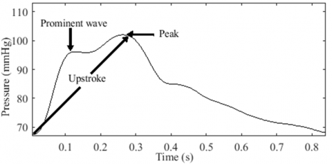
The typical pulse in AS is referred to as anacrotic, derived from the term "anadicrotic," meaning twice beating on the upstroke [20]. It indicates the presence of two waves during systole. However, this statement creates confusion regarding whether the first wave represents the percussion wave of the bisferiens pulse or the anacrotic wave of the anacrotic pulse [38]. This confusion arises when the first wave has a lower peak compared to the second wave, as illustrated in Figure 10.
Fleming [39] described the peaks in the bisferiens pulse as twin peaks. This is visually evident due to their brisk appearance in time [40]. In contrast, anacrotic pulses lack this suddenness. Instead, the upstroke seems interrupted by a notch, resulting in a small first wave, followed by a longer duration to reach the peak of the second wave. This explains Fleming's description of the second wave as being taller and broader than the first wave [39]. Thus, the shape and depth of the dip between the two peaks help differentiate between anacrotic and bisferiens pulses, as they depend on the magnitude of the two waves [41].
Figure 10. A confusing double peaked pulse
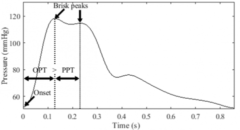
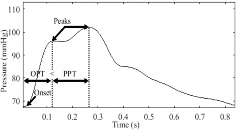
Temporal analysis. Considering the temporal aspect, our analysis demonstrates that the two waves appear briskly when the peak-to-peak time (PPT) is shorter than the onset-to-peak time (OPT) (Figure 11 (a)). Conversely, the tidal wave appears larger when the PPT is longer than the OPT (Figure 11 (b)). Hence, it is reasonable to assume that the anacrotic pulse has a longer PPT than the OPT.
(a) Brisk peaks in a bisferiens pulse
(b) Broad tidal wave in anacrotic pulse
Figure 11. Bisferiens and anacrotic pulses comparaison
Contour analysis. We define anacrotic pulses associated with a non-prominent anacrotic wave based on two conditions:
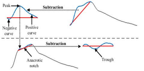
Firstly, we set a line connecting the onset and peak of the pulse, and then we subtract the upstroke curve from this line. This subtraction generates a subtracted curve (SC) comprising positive and negative samples. The positive samples represent the curve above the line, while the negative samples represent the curve below the line. Consequently, for an anacrotic wave to be present, the area under the positive curve (AUPC) must be greater than the area under the negative curve (AUNC).
Secondly, we locate the peak value of the SC, which represents the positive inflection point of the wave. We then set another line connecting the inflection point and the pulse peak. The trough in the secondary SC represents the notch of the anacrotic pulse.
Figure 12 provides a further illustration of the detection process.
Figure 12. Anacrotic pulse characteristics detection
2.6.3 Dicrotic model
In contrast to bisferiens and anacrotic pulses, a dicrotic pulse is characterized by the presence of two waves, with the first wave occurring during systole and the second wave during diastole.
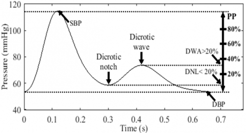
Contour analysis. Meadows et al. [22] defined a fully dicrotic pulse as having a dicrotic wave amplitude (DWA) greater than 30% of the PP and a dicrotic notch level (DNL) less than 10% of the PP. They also established borderline criteria, which include a DWA greater than 20% of the PP and a DNL less than 20% of a PP. However, it's important to note that a low level of the dicrotic notch does not necessarily indicate a large dicrotic wave. Therefore, pulses with low DNL and high DWA are labeled as dicrotic pulses, while pulses with only low DNLs are labeled as deep pulses. In this study, we employ the borderline criteria to model dicrotic and deep pulses, as illustrated in Figure 13.
Figure 13. Borderline dicrotic pulse criteria
2.6.4 High amplitude models
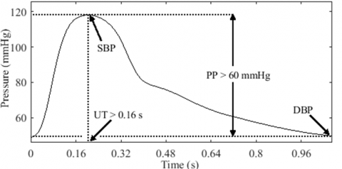
The amplitude of a pulse can be understood in terms of volume or pressure [42]. The specific interpretation depends on the type of pulse and the nature of the study. In our study, we focus on arterial pressure pulses, and thus we refer to the amplitude as PP. The normal range for PP is considered to be between 40 mmHg and 60 mmHg [43]. Therefore, a high amplitude pulse (HAP) is defined as having a PP greater than 60 mmHg. Our analysis includes three types of HAP models: bounding pulse (BDP), shallow HAP, and water hammer pulse (WHP).
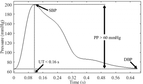
(1) The BDP is characterized by a rapid rise in pressure, resulting in a steep upstroke, as illustrated in Figure 14. To our knowledge, there are no defined cutoff values or guidelines to determine the normal range of upstroke time (UT). However, Wood [20] proposed that an UT of less than 0.16 s can be considered normal. In line with Wood's criterion, Boiteau et al. [44] reported a normal radial UT ranging between 0.11 s and 0.16 s. Thus, we define a BDP as having a PP greater than 60 mmHg and an UT less than or equal to 0.16 s.
Figure 14. Bounding pulse model
(2) We refer to the second type of HAP as shallow due to its inclined upstroke, late systolic peak, and occasional early hump. This pulse pattern is commonly observed in conditions associated with arterial stiffness [45]. Similarly, in the case of bradycardia (slow heart rate), the pulse displays a prolonged time in reaching the peak, leading to a broad peak, as illustrated in Figure 15. In contrast to the BDP, a pulse is considered shallow when its UT exceeds 0.16 s.
Figure 15. A high amplitude pulse with a slow upstroke
(3) As pointed out in the first section, the BDP can be observed in various physiological and pathological states [19]. Particularly, a unique bounding quality often occurs in moderate to severe AR states known as a WHP, which is mostly marked in peripheral arteries [46]. As revealed long ago, the main characteristics that distinguish WHP from other HAPs are its sudden upstroke, narrow and wide percussion wave, and preferably flattened tidal and dicrotic waves [47]. In response to these signs, we propose three interpretation criteria to identify a WHP:
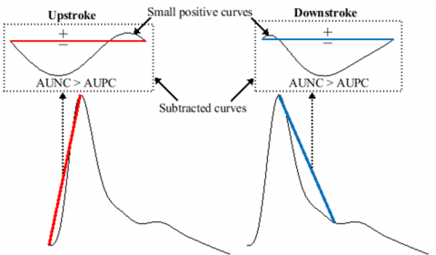
Contour analysis. In accordance with the aforementioned signs, most researchers define a WHP by a steep upstroke, sharp or narrow percussion wave, wide pulse pressure, collapsing, and a sharp downstroke [25, 41, 46, 48]. Therefore, sharpness is an important feature in defining the WHP. Estimating the degree of sharpness in the pulse has been suggested in the literature [49]. However, assessing the sharpness of the WHP requires considering the entire systolic wave, which includes a sharp systolic upstroke and downstroke. To achieve this, we establish two lines: the first line extends from the onset to the peak (upstroke), while the second line extends from the peak to the dicrotic notch (downstroke). The proximity of the wave to these lines indicates its sharpness. Thus, a pulse is considered sharp if the AUNC is greater than the AUPC for both the systolic upstroke and downstroke, as illustrated in Figure 16. Similarly, we define a flat diastolic portion if its corresponding AUNC is greater than or equal to its AUPC.
Figure 16. Sharp systolic wave from a water hammer model
Amplitude. McGee [48] stated in his book that a PP equal to or greater than 80 mmHg and a DBP equal to or less than 50 mmHg increase the probability of moderate to severe AR. These benchmarks were established based on studies investigating the correlation between the severity of AR and PP [50] as well as DBP [51]. Although the WHP is primarily a systolic phenomenon that is not directly defined by low DBP [25], setting this condition up enhances the likelihood of its manifestation. This has been confirmed by elevating the arm of patients diagnosed with AR, resulting in a decrease in their DBP and a more pronounced water hammer quality [46-48].
Temporal analysis. Boiteau et al. [44] emphasized that the UT in normal individuals is shortened and does not significantly differ from that observed in AR cases. However, upon further examination of the UT and systolic time (ST) measurements in their study, we observed that some AR subjects had UT values below the normal range reported in their study (0.11 s to 0.16 s). Interestingly, all AR subjects with UT values below 0.11 s had UTs that were less than one third of the ST (UT/ST < 34%), while the majority of the remaining subjects had UTs that were less than half of the ST [44]. Based on this observation, it is reasonable to assume that a short UT, particularly one that is less than one third of the ST, may be indicative of the suddenness in the upstroke of the WHP. Furthermore, the ST is another important feature in identifying a WHP, as it is typically prolonged in AR conditions, ranging between 0.28 s and 0.4 s [44].
Figure 17. Pulsus tardus characteristics
2.6.5 Tardus model
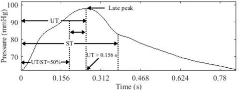
A slow-rising pulse, known as pulsus tardus, is characterized by a delayed peak and is sometimes referred to as pulsus parvus et tardus when associated with low amplitude (Figure 17). People with AS have pulsus tardus, and its slanted upstroke can look smooth or be broken up by a notch [52], as was shown before in the anacrotic pulse.
Temporal analysis. We define pulsus tardus as having an UT greater than 0.156 s, based on a study conducted by Yoshioka et al. [53], in which the authors concluded that an UT exceeding 0.156 s indicates severe AS. In certain cases, pulsus tardus can be mistaken for a shallow HAP, as it can be associated with a high PP in the radial artery due to arterial stiffness [53]. Therefore, we define the pulsus tardus model as having an UT longer than the remaining ST, with an UT/ST ratio greater than 50%, as illustrated in Figure 17.
This definition is supported by the observation that the systolic peak in pulsus tardus often occurs near the second sound of the heart, which represents the closure of the aortic valve at the end of the systolic phase [19].
Amplitude. The term "parvus" is used to describe a pulse with low volume [54] or a narrow PP [55]. In the context of pulse pressure, researchers investigated PP measurements in AS states to determine whether pulsus parvus is indicative of severe AS [53]. Thus, a narrow pulse pressure is one of the defining features of pulsus parvus. Accordingly, we define a narrow PP as being less than 40 mmHg [43]. Therefore, pulsus parvus et tardus shares the same characteristics as pulsus tardus, except for the presence of a narrow PP.
2.7 Class labels
Table 1 and Table 2 provide an overview of the parameters used in the modeling process of AAPs. Table 1 presents the contour parameters, while Table 2 outlines the time and amplitude parameters.
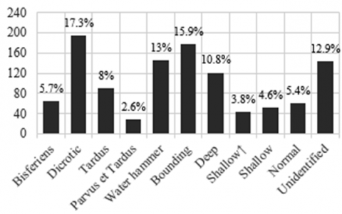
The modeling process involved a total of 1120 records. Analysis of the obtained records revealed a prevalence of similar pulse models, as depicted in Figure 18. All the resulting models were classified individually, except for the anacrotic models. Due to their limited occurrence, the anacrotic pulses were categorized under the tardus class. Similarly, anacrotic pulses featuring low amplitude were categorized under the parvus et tardus class.
Furthermore, an additional model named "shallow pulse" was introduced to reduce the number of cases falling under the unidentified class. As indicated in Table 2, the shallow pulse shares similar features with the shallow HAP model except for the high amplitude. Figure 19 displays the sample size distribution among the different classes, with each sample representing a group of models derived from a specific record.
Figure 18. AAP modeling results taken from different ABP records
Figure 19. AAP classes sample size
Table 1. Pulse contour parameters used in AAP modeling process
|
Pulse |
DNL (%) |
DWA (%) |
USC |
DSC |
P Wave |
T Wave |
D Wave |
|
Normal |
≥ 20 |
> 20 |
NS |
NS |
Prominent |
Non-prominent |
Prominent |
|
Bisferiens |
NS |
NS |
NS |
NS |
Prominent |
Prominent |
NS |
|
Anacrotic |
NS |
NS |
AUPC > AUNC |
NS |
Either |
Prominent |
NS |
|
Dicrotic |
< 20 |
> 20 |
NS |
NS |
Prominent |
None |
Prominent |
|
Deep |
< 20 |
≤ 20 |
NS |
NS |
Prominent |
None |
NS |
|
Water hammer |
NS |
NS |
AUPC < AUNC |
AUPC < AUNC |
Prominent |
Non-prominent |
Non-prominent |
Notes: 1. NS: Not specified. 2. P: Percussion. 3. T: Tidal. 4. D: Dicrotic. 5. USC: Upstroke subtracted curve. 6. DSC: Downstroke subtracted curve.
Table 2. Time and amplitude parameters used in AAP modeling process
|
Pulse |
UT (s) |
ST (s) |
UT/ST (%) |
PP (mmHg) |
DBP (mmHg) |
|
Normal |
≤ 0.16 |
≥ 0.28 |
< 50 |
≤ 60 |
NS |
|
Bounding |
≤ 0.16 |
≥ 0.28 |
≤ 50 |
> 60 |
NS |
|
Shallow ↑ |
> 0.16 |
NS |
≤ 50 |
> 60 |
NS |
|
Water hammer |
≤ 0.11 |
≥ 0.28 |
< 34 |
≥ 80 |
≤ 50 |
|
Shallow |
> 0.16 |
NS |
≤ 50 |
≤ 60 |
NS |
|
Tardus |
> 0.156 |
≥ 0.28 |
> 50 |
≥ 40 |
NS |
|
Parvus et tardus |
> 0.156 |
≥ 0.28 |
> 50 |
< 40 |
NS |
|
Anacrotic |
PPT > OPT |
NS |
NS |
NS |
NS |
Note: ↑: High amplitude.
2.8 Feature extraction and data preparation
Before extracting features, a subset comprising 40% of the pulses was selected from each PPG signal. From each pulse, a set of 24 features was extracted for use in our classification system. Our analysis begins by selecting six segments from the pulse signal, including the total pulse (Figure 20). Each segment is then processed to derive four distinct features.
Figure 20. Features extraction from a PPG pulse signal
The first feature relates to the temporal aspects of the selected phases and is defined as:
$F_T=\frac{p h}{f S}$ (15)
where, FT represents the time feature, ph denotes the length of the selected phase, and fs corresponds to the sampling frequency.
Next, we determine the slope features by establishing lines that connect the limits of each curve within the selected segments. The slope is calculated using the following equation:
$F_{S L}=\frac{Y_{\text {end }}-Y_{i n}}{p h-1}$ (16)
where, FSL represents the slope feature, while Yin and Yend denote the data values marking the beginning and end of a given segment in the PPG signal.
Finally, we explore the SCs obtained by subtracting each curve from its corresponding line. These SCs are represented as a sequence of data points:
$C_{\text {sub }}=\left\{v_1, v_2, v_m, \ldots \ldots v_M\right\}$ (17)
where, v is the expected data value from a given sample index m, and M is the length of the data points.
We then calculate the mean and kurtosis of the SCs. The mean represents the average value of the SC:
$F_M=\frac{1}{M} \sum_{m=1}^M v_m$ (18)
The kurtosis measures the tailedness of the SC is defined as:
$F_{K R}=\frac{\frac{1}{M} \sum_{m=1}^M\left(v_m-F_M\right)^4}{\left(\frac{1}{M} \sum_{m=1}^M\left(v_m-F_M\right)^2\right)^2}$ (19)
As a result, we present the input matrix Fin as follows:
$F_{\text {in }}=\left[\begin{array}{ccccc}f_1(1) & f_1(2) & f_1(u) & \ldots & f_1(U) \\ f_2(1) & f_2(2) & f_2(u) & \ldots & f_2(U) \\ \vdots & \vdots & \vdots & & \vdots \\ f_W(1) & f_W(2) & f_W(u) & \ldots & f_W(U)\end{array}\right]$ (20)
where, u∈{1, 2…, 24} denotes a specific feature in a row matrix, U represents the twenty fourth feature while W is the length of the input dataset.
To complete the data preparation, we assign class labels to each row of the input matrix based on its corresponding AAP class. Next, we divide the input data into an 80% training set and a 20% test set. This division enables the classifiers to be trained on a majority of the data and evaluate their performance on unseen data during testing.
To address potential biases resulting from class imbalance, a data balancing process is applied to the training set. This involves oversampling the classes with low datasets by duplicating their instances until they reach a similar size to the class with the highest number of samples. This prevents the training model from favoring classes with larger datasets.
2.9 Classification algorithms
Unlike other disciplines, explainability is paramount for Artificial intelligence (AI) in healthcare [16]. While DNNs might offer impressive performance, their internal complexity challenges interpretation [56]. For explainable AI (XAI) researchers investigating the communication of clinical AI logic and reasoning, algorithms with more transparent internal representations are preferable. By selecting ML techniques that retain a certain interpretability degree of internal processes, XAI researchers can better systematically explore, evaluate, and clearly explain models' functioning.
2.9.1 Parametric models
Parametric models, by design, often have a simpler and more transparent structure [57]. The relationship between variables is explicitly defined by a set of parameters. However, the simplicity of parametric models may limit their ability to capture complex and nonlinear relationships present in the PPG signals. For instance, NB assumes that features are conditionally independent, given the class label [58]. This assumption might not hold in tasks involving physiological signals like PPG, where features might have complex interdependencies. Similarly, discriminant analysis classifiers assume that the features follow a specific distribution within each class [59].
2.9.2 Non-parametric models
In contrast, non-parametric models are more flexible and can capture complex relationships in the data without relying on strong assumptions. DTs are non-parametric models that can handle non-linear relationships between variables. This type of algorithm offers high interpretability as its decision-making process is based on a sequence of explicit rules that form a hierarchical structure [60]. However, training a single DT with a relatively large dataset might lead to deeper or more complex trees, which could potentially compromise interpretability and increase the risk of overfitting. Ensemble methods like bagging, which combine multiple DTs, might offer better performance while retaining interpretability to a certain extent. BT involves training multiple DTs on different subsets of the training data and combining their outputs to make predictions [31]. This reduces the variance of individual trees and helps mitigate overfitting [32].
KNN is another example of a non-parametric model. It is known as a "lazy learning" or "instance-based learning" algorithm because it doesn’t involve explicit training or building a model in the same way as many other algorithms [30]. It basically stores all available training cases and classifies new cases by assigning them to similar classes as the closest cases (neighbors) in the training set. The idea is simple: cases near each other have the same features [61]. For this purpose, only two parameters are needed: the number of neighbors (K) in the training set and the formula that calculates the distances (distance metric) between a new case (query point) and K-neighbors. The city block (Manhattan distance) is a simple distance metric that could be used for distance measuring. The distance between two points X and Y in a D dimensional space is calculated as:
$\operatorname{CityBlock}(X, Y)=\underset{i=1}{D}\left|X_i-Y_i\right|$ (21)
To better improve the query point outcome, weights could be assigned to the neighbors so that the nearest one will have more influence on the output class [61]. The weight for each neighbor in KNN can be calculated using the inverse of the square root of the distances:
Weights $(X, Y)=\frac{1}{\sqrt{\operatorname{CityBlock}(X, Y)}}$ (22)
2.9.3 Proposed experiment
As non-parametric classifiers, KNN and BT provide intuitive approaches for nonlinear problems due to their simple structure, compared to other complex classifiers like SVM [62] or DNN [56]. Meanwhile, this nonlinear flexibility could offer higher performance compared to parametric models while retaining a certain degree of simplicity. Accordingly, we validated the efficacy of the BT and KNN classifiers by comparing them with other classifiers. This included both parametric and non-parametric models, such as NB, Linear Discriminant analysis (LDA), SVM, and DT. MATLAB’s classification learner toolbox was used to train the models using a subset of the original dataset.
Next, we explored different KNN and BT models with varied K values and learners (DTs), respectively. The most performing KNN and BT models were re-trained and re-tested using the entire dataset. To stabilize the model's performance, the k-fold cross-validation technique was employed by randomly splitting the data into 10 equally sized groups (folds). Within each iteration, 9 folds are used for training, and the remaining 1-fold is used for validation. The process was repeated 10 times, and the results from each iteration were averaged to determine the overall accuracy of the model.
2.9.4 Evaluation metrics
Different metrics are used to evaluate the performance of the classification system, including sensitivity (SE), specificity (SP), precision (PR), accuracy (AC), and F1 score (F1), and are defined as follows:
$S E=\frac{T P}{T P+E N}$ (23)
$S P=\frac{T N}{T N+F P}$ (24)
$P R=\frac{T P}{T P+F P}$ (25)
$A C=\frac{T P+T N}{T P+F P+T N+F N}$ (26)
$F 1=\frac{2(S E \times P R)}{(S E+P R)}$ (27)
where, TP represents true positives, which are instances correctly identified as positive. TN represents true negatives, which are instances correctly identified as negative. FP represents false positives, which are instances incorrectly classified as positive. FN represents false negatives, which are instances incorrectly classified as negative.
3.1 Dataset development
The data preparation aimed at providing labeled PPG features to create a dataset that enabled proceeding with the ML-modeling experiments. The dataset was developed by extracting sets of 24 features from pre-segmented PPG pulses. The PPG-ABP pulses were extracted from the 1120 1-minute signals using a third derivative approach that uses LMTDs to approximate the troughs. Afterward, the pulses were fed into an optimizer to locate their dicrotic notches.
To capture meaningful physiological variations, features were extracted by identifying changes that occur at specific cardiac cycle landmarks. The pulse onset (initial trough) reflects the beginning of the cycle. The peak signifies mid-systole. The dicrotic notch indicates the end-systole and start of diastole. The offset (latter trough) highlights the end of the cycle. Segmenting the pulse at these cardiac landmarks yielded six distinct sub-waves, each of which describes a particular cardiac event.
Mathematically, pulse morphology changes represent statistical variations affecting waveform segments over time. Considering each segment as a normal distribution, kurtosis describes the extension of waveforms in the tail regions compared to normal. The mean indicates a central tendency. Slopes measure the waveform angle of inclination.
Ultimately, four metrics—kurtosis, mean, slope, and time—characterized feature morphologies. Measurements were taken from each segment, yielding 24 features per pulse (6 segments × 4 metrics). Only 40% of pulses from single 1-minute signals were analyzed. The features were then assigned to 11 class labels created via a modeling process applied to pre-segmented ABP pulses. This involved characterizing the amplitude, contour, and temporal profiles of key AAP types. In total, the final dataset contained 24 × 47,000 samples.
3.2 Machine learning modeling
We evaluated several machine learning models in MATLAB R2020a, including NB, LDA, SVM, KNN, DT, and BT. These classifiers were integrated into the software's classification learner toolbox. Models were developed using a subset of 27,000 samples from the full dataset, labeled with 11 classes. 80% of the data was used for training, and the remaining 20% was for testing. As shown in Table 3, KNN and BT substantially outperformed other models in terms of training accuracy, time, prediction speed, and test accuracy. This demonstrates their effectiveness in addressing multiclass challenges and nonlinear relationships within the dataset.
Table 3. Models comparison
|
Results |
KNN |
BT |
DT |
LDA |
SVM |
NB |
|
Training accuracy (%) |
98.2 |
97.7 |
69.7 |
59.6 |
61.5 |
54.3 |
|
Training time (sec) |
79 |
11 |
9 |
8 |
1722 |
8 |
|
Prediction speed (obs/sec) |
2000 |
69000 |
210000 |
130000 |
6800 |
87000 |
|
Test accuracy |
92.5 |
90.2 |
67.5 |
61.5 |
35.6 |
57 |
Notes: 1. obs: observation (data point). 2. sec: second.
Based on the results in Table 3, LDA and NB provided efficient computation times of 8 seconds and prediction speeds up to 210,000 observations per second. However, their training and test accuracies were relatively low, likely due to inconsistencies between their underlying assumptions and the actual data distribution. This confirms that parametric models struggle with nonlinear relationships in the data. SVM training took 1722 seconds to achieve only 61.5% and 35.6% for training and test accuracy, respectively. In addition to its computational complexity, SVM seems to overfit the data. Decision trees appeared to learn meaningful patterns in only 9 seconds but resulted in relatively low accuracies as well. Overall, the results indicate that the models failed to handle the multiclass problems effectively. With more classes, there is less average training data per class, making class boundaries harder to learn accurately.
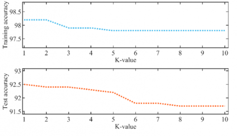
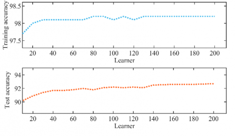
To further analyze KNN and BT, we tuned their hyperparameters. K values for KNN ranged from 1 to 10, and learners for BT increased from 10 to 200. Figure 21 shows how training and test accuracy evolved with these hyperparameters.
As Figure 21(a) depicts, KNN training and test accuracy progressively decreased as K increased, indicating optimal performance with a single neighbor to separate the 11 classes. This emphasizes the fact that simpler KNN models can achieve more accurate results. In contrast, Figure 21(b) shows BT required 200 learners to reach the best accuracy, emphasizing that more complex models suit multiclass problems better. In summary, hyperparameter tuning validated KNN and BT suitability for these nonlinear, multiclass challenges.
(a) K-value variation versus accuracies
(b) Learner variation versus accuracies
Figure 21. Training a test accuracies evolution against KNN and BT hyperparameters
3.3 Classification results
In this study, we developed a PPG-based classification system aimed at predicting various AAPs. For this purpose, MATLAB’s classification learner app was used to train and validate the KNN and BT classifiers using a dataset sized 24 x 47,000 samples. In accordance with the tuning process, the KNN model was created by setting K = 1, while the BT model was created by setting the number of learners at 200. The proposed methodology exhibited good performance for both the BT and KNN classifiers, as indicated in Table 4.
Table 4. Classification results
|
Training Accuracy (%) |
Test Accuracy (%) |
||
|
BT |
KNN |
BT |
KNN |
|
97.6 |
97.5 |
91 |
90.9 |
The BT model achieved an overall training accuracy of 97.6%, while the KNN model achieved 97.5%. The corresponding testing accuracies were 91% for the BT model and 90.9% for the KNN model. It is evident that the BT classifier outperformed the KNN classifier, although both classifiers proved to be effective predictors of AAPs.
However, evaluating the reliability of an ML model relies on analyzing its testing performance. Additionally, it is essential to analyze each class individually to gain a more insightful assessment of the system, particularly when dealing with multiple classes and achieving high overall testing accuracy. In such cases, metrics such as specificity and accuracy, which incorporate TN classes, tend to yield high values (Table 5). Alternatively, metrics such as sensitivity, precision, and F1 score offer more appropriate measures for individual assessment.
Specifically, the BT model achieved a sensitivity, precision, and F1 score of 95.1%, 96.2%, and 95.6% for the 'deep' class, while the KNN model achieved a sensitivity, precision, and F1 score of 95.7%, 95.4%, and 95.6% for the same class. Conversely, the 'shallow↑' class exhibited the lowest values for the BT model, with a sensitivity, precision, and F1 score of 83.7%, 85.4%, and 84.5%, respectively. Similarly, the 'parvus et tardus' class displayed the lowest values for the KNN model, with a sensitivity, precision, and F1 score of 84.8%, 84.8%, and 84.8%, respectively.
Furthermore, classes such as 'dicrotic', 'bisferiens', 'shallow', and 'tardus' demonstrated performance values close to those of the 'deep' class for both models. Conversely, classes such as 'water hammer', 'bounding', and 'normal' showed performance values close to those of the 'shallow↑' and 'parvus et tardus' classes. These findings suggest that both models consistently perform well and exhibit comparable performance across different classes, indicating their capabilities as AAP detectors.
3.4 System design
Table 6 overviews different approaches used to create CVD systems, presenting their outputs, related pathologies, classifiers, input features, as well as their accuracies. The main advantage of the current system is its multitasking abilities, as evidenced by the related pathologies. However, transparency is also crucial in healthcare systems. This requires balancing performance and simplicity at both the modular and instance levels. While previous studies achieved good accuracy, their features and models involved complex trade-offs.
Particularly, heuristic and transformational feature extraction techniques in studies [9-11, 14-15, 26] provided abstract representations that could be difficult to justify in a clinical context. For instance, algorithms like swarm intelligence [14] and transformations [9, 15] often involve intricate mathematical operations or optimization techniques. Besides, classifiers such as SVM, ANN, Gaussian Mixture Model (GMM), and Bidirectional Long Short-Term Memory (BLSTM) may compromise modular simplicity.
For example, DNNs like BLSTM operate as black-box models, making it challenging to explain predictions [56]. Similarly, Multi-layer perceptron (MLPs) and ANNs can be complex, with many hidden layers and neurons. SVMs can add complexity as well [62], especially with non-linear kernels. GMMs also increase in complexity with more components and high-dimensional data [63]. However, the LR and NB models created by Prabhakar et al. [14] offer interpretability through their parametric nature. Unfortunately, dimensionally reduced features introduce instance-level trade-offs.
The present work used physiological PPG morphology features extracted from time, slope, and SCs to describe pulse shape characteristics. This resulted in a 24-feature set, which is reasonable given the multiple classes involved. In terms of complexity, the KNN model was designed with simpler hyperparameters, requiring a single neighbor for multi-class prediction. However, relying solely on the closest data point could lead to erratic predictions if that point is an outlier. Conversely, using 200 learners for the BT model undermines its simplicity, despite incorporating interpretable individual models. Tuning parameters exclusively for performance may thus trade off simplicity.
Table 5. Test performance
|
Classes |
Sensitivity (%) |
Specificity (%) |
Precision (%) |
Accuracy (%) |
F1-Score (%) |
|||||
|
BT |
KNN |
BT |
KNN |
BT |
KNN |
BT |
KNN |
BT |
KNN |
|
|
Bisferiens |
93 |
92.3 |
99 |
99.3 |
89.8 |
92.3 |
98.5 |
98.6 |
91.4 |
92.3 |
|
Dicrotic |
94.9 |
94 |
98.6 |
98.4 |
94.5 |
93.9 |
97.8 |
97.5 |
94.7 |
93.9 |
|
Tardus |
91.7 |
91.3 |
98.9 |
99.2 |
86.6 |
90 |
98.3 |
98.6 |
89.1 |
90.6 |
|
Parvus et tardus |
83 |
84.8 |
99.8 |
99.6 |
92.8 |
84.8 |
99.4 |
99.2 |
87.7 |
84.8 |
|
Water hammer |
87.8 |
89.1 |
98.2 |
98.1 |
88.3 |
87.7 |
96.8 |
96.8 |
88.1 |
88.4 |
|
Bounding |
86.8 |
86 |
98.1 |
98.3 |
88.8 |
90 |
96.4 |
96.5 |
87.8 |
88 |
|
Deep |
95.1 |
95.7 |
99.3 |
99.2 |
96.2 |
95.4 |
98.7 |
98.6 |
95.6 |
95.6 |
|
Shallow ↑ |
83.7 |
84.2 |
99.6 |
99.6 |
85.4 |
85.9 |
99.1 |
99.1 |
84.5 |
85.1 |
|
Shallow |
92 |
94.4 |
99.5 |
99.4 |
89.2 |
88.8 |
99.1 |
99.2 |
90.5 |
91.5 |
|
Normal |
86.1 |
85.1 |
99.5 |
99.4 |
89.2 |
86.6 |
98.9 |
98.7 |
87.6 |
85.9 |
|
Unidentified |
90.9 |
90.5 |
98.6 |
98.5 |
90.1 |
89.4 |
97.6 |
97.5 |
90.5 |
90 |
Table 6. Comparative results relative to prior studies
|
Study |
Classification Output |
Input Features |
Related Pathologies |
Classifier |
Accuracy |
|
Putra et al. [10] |
Healthy vs. CHD |
Frequency band features and statistical features |
• Coronary Heart Disease |
KNN |
90.9% |
|
Hackstein et al. [11] |
Control Group vs. Aneurysms |
Parameter estimation of ARMAX models and frequency response features |
• Aneurysms |
KNN |
60% |
|
Hosseini et al. [12] |
High Risk CAD vs. Low Risk CAD |
Statistical, time-interval and time-domain features |
• Coronary Artery Disease |
KNN |
81.5% |
|
De Moraes et al. [13] |
Cardiopathies vs. Healthy |
Time domain and statistical features |
• Idiopathic Dilated Cardiomyopathy • Chagas Cardiomyopathy • Ischemic Cardiomyopathy |
KNN MLP K-means SOM |
88.57-100% 90-100% 91.85-100% 87.5-100% |
|
Ramachandran et al. [15] |
Cardiac-risk level 1 vs. Cardiac- risk level 2 vs. Respiratory disorder vs. Normal |
Statistical features, DWT coefficients, dimensionally reduced features via SVD |
• Risk assessment |
GMM SDC |
96.64 97.88% |
|
Prabhakar et al. [14] |
CVD-risk vs. Normal |
Dimensionally reduced features via metaheuristic optimization algorithms |
• Risk assessment |
LR SVM NB ANN |
99.48% 98.96% 98.96% 98.96% |
|
Palanisamy and Rajaguru [9] |
CVD-risk vs. Normal |
Dimensionally reduced features via heuristic- and transformation-based techniques |
• Risk assessment |
HS |
98.31% |
|
Tjahjadi et al. [26] |
Hypertension vs. Pre-hypertension vs. Normotension |
Time-Frequency analysis |
• Hypertension |
BLSTM |
93% |
|
Tjahjadi and Ramli [61] |
Hypertension vs. Pre-hypertension vs. Normotension |
2100 PPG samples |
• Hypertension |
KNN |
93% |
|
This study |
9 AAPs vs. Normal vs. Unidentified |
Statistical and time-domain morphological features |
• Hypertrophic obstructive cardiomyopathy • Aortic stenosis • Aortic regurgitation • Mixt valvular diseases • Pulmonary embolism • Constrictive pericarditis • Pericardial tamponade • Cardiomyopathies • Arteriovenous fistula • Sepsis • Anemia • Thyrotoxicosis • Severe bradycardia |
KNN BT |
90.9% 91% |
3.5 Pulse wave features
In our research, we relied on pulse signal segmentation to extract PPG features, a process facilitated by the implementation of our proposed trough and dicrotic notch detectors. This was particularly important given that a significant number of signal records exhibited undetectable dicrotic notches and troughs.
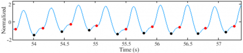
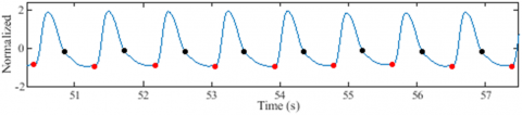
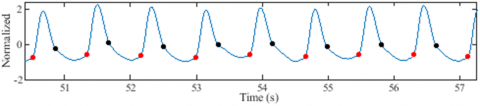
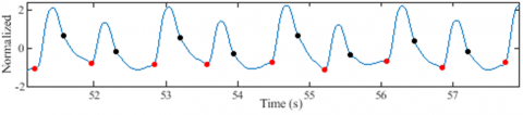
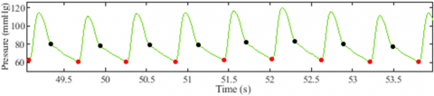
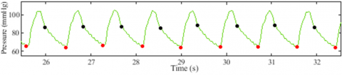
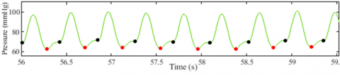
Similarly, the precise detection of troughs and dicrotic notches proves indispensable in obtaining key measurements such as UT, ST, PP, DBP, AUNC, AUPC, DNL, DWA, OPT, and PPT, all of which contribute to the proposed AAP models. Figure 22 presents some segments of ABP and PPG signals resulting from the application of the proposed detectors. The results demonstrate the algorithm's efficiency in detecting suppressed troughs and dicrotic notches.
Visual inspection alone is not enough to judge how well these detectors work, even though Figure 22 shows that the proposed algorithms can find suppressed troughs and dicrotic notches. The human physiology is inherently dynamic over time [29], leading to the dynamic occurrence of pulse wave features within each cardiac cycle.
(a) Suppressed troughs in a PPG signal
(b) Suppressed dicrotic noches in a PPG signal
(c) Suppressed troughs and dicrotic noches in a PPG signal
(d) A disturbing PPG signal with suppressed troughs and dicrotic notches
(e) Suppressed dicrotic notches in a ABP signal
(f) Suppressed dicrotic notches in an ABP signal
(g) Suppressed troughs in an ABP signal
Figure 22. Dicrotic notch and trough detection results
Visual inspection alone is not enough to judge how well these detectors work, even though Figure 22 shows that the proposed algorithms can find suppressed troughs and dicrotic notches. The human physiology is inherently dynamic over time [29], leading to the dynamic occurrence of pulse wave features within each cardiac cycle.
Consequently, we introduced the SD metric to capture the variation of dicrotic notches throughout the entire signal during the evaluation process. The underlying idea behind the SD metric was to ensure temporal consistency in the prevalence of dicrotic notches within a signal record. By making sure this condition is met, the dicrotic notches stay in place even when the signal has different morphological pulse patterns, as seen in Figure 22(d).
Similarly, the SD metric can be applied to evaluate the detected troughs by considering the variation in the length of pulses within a signal. To provide quantitative insight into the performance of the detectors, Table 7 displays the average SD values for both detectors, derived from the analysis of over 200 records during the detection procedures.
Table 7. Average of SD value results
|
Dicrotic Notch |
Trough |
||
|
PPG |
ABP |
PPG |
ABP |
|
1.22 |
0.94 |
1.75 |
1.56 |
Notably, the parameters employed in trough and dicrotic notch detection are specific for signals with an Fs=125 Hz, as in the MIMIC databases [29, 35]. Hence, further analysis is necessary when applying our detection methodology to signals with higher sampling frequencies.
3.6 Clinical perspectives
The proposed classification system holds potential as an inexpensive assistant tool in clinical settings. Its ability to detect individual AAPs, which may be indicative of specific disease states, makes it particularly valuable. For instance, the identified AAPs, such as pulsus tardus, pulsus parvus et tardus, bisferiens pulse, and water hammer pulse, could aid in detecting several VHDs [25, 52, 53]. Similarly, the presence of a dicrotic pulse may suggest conditions related to low cardiac output [21, 22]. A deep pulse, on the other hand, could be indicative of sepsis or low peripheral resistance [23, 24]. Moreover, conditions such as anemia, thyrotoxicosis, severe bradycardia, AR, or arteriovenous fistula are typically associated with a bounding pulse or a slow bounding pulse, which we referred to as shallow HAP [19].
Although AAPs have been historically linked to specific CVDs [18, 20, 22, 38, 39, 47], there are no precise hemodynamic standards to identify their morphological states. Clinicians often use AAP morphological terms only when there is an association with particular CVDs. For instance, terms such as pulsus tardus, parvus et tardus, and anacrotic are frequently utilized in the analysis of AS tracings [20, 53]. Similarly, terms like bisferiens, water hammer, and bounding are commonly employed when examining AR tracings [25, 46]. Additionally, the radial artery is thought to be the best way to get ABP signals, but there isn't a lot written about the hemodynamic features that define the normal morphological state of the radial pulse. Currently, the criteria used involve visual examination of pulse signals or palpation of an artery [19].
In light of this, we sought to develop a modeling process to identify AAP patterns, relying on three interpretations, including contour, amplitude, and temporal analysis. For the contour analysis, criteria, theories, and descriptions from studies on AAP morphologies had to be taken into account. This let the right contour parameters be found. The amplitude and temporal analysis, on the other hand, used criteria and hemodynamic measurements from relevant pathological studies that were known to show up with those shapes. This enabled us to generate the time and amplitude parameters for the AAP models.
Linking morphologies to specific CVDs based on known hemodynamic mechanisms could make doctors more confident in assessments compared to systems that don't have likely causes. This offers promise as a practical, affordable clinical monitoring and screening tool. By integrating it into wearable biosensing devices [8], it could enable several benefits:
(1) Doctor assistance: Direct doctor intervention if CVD is suspected, as they could non-invasively verify abnormalities and view diseases commonly associated with a patient's morphological profile.
(2) Surgery assistance: Post-surgery follow-ups, allowing doctors to remotely monitor patients dismissed from the clinic via a connected patient portal within the Electronic Health Record (EHR). This could aid recovery oversight and early intervention if issues arise.
(3) Nursing assistance: By setting automated alerts for any abnormalities detected in a patient's pulse patterns (AAPs).
(4) Timely notifications: Any concerning patterns would trigger alerts to patients and clinicians to act promptly if needed.
However, successful clinical integration depends on addressing some potential challenges:
(1) Motion artifact susceptibility: PPG is sensitive to motion artifacts [36]. Automatic rejection of corrupted signals using techniques like the skewness signal quality index (SSQI) can help minimize motion interference [64]. Customizable reminders or strategic sensor placement in less-prone body locations could also be explored to reduce motion artifacts.
(2) System update: Ongoing clinically annotated ABP/AAP data collection is needed to refine the model over time, but guidelines and dedicated collection programs are currently lacking. To solve this, awareness must be raised among biomedical engineers about the need to collaborate with clinics to facilitate data collection programs. Beyond clinics, smartwatch/fitness band integration could foster global health awareness alerts.
(3) Explainability: Gaining physician and patient trust requires explainable model predictions [16]. Interactive tools can demonstrate prediction logic by linking patient pulse patterns to animations of corresponding hemodynamics. For example, visualize patterns alongside diagrams of associated processes. Inputs can also be adjusted in "what if" scenario simulations, where users can manipulate feature values and see how the predicted risk or disease changes in response. Together, visualization and simulation approaches elucidate models grounded in medical evidence, fostering trust through transparency.
This study introduced a novel, non-invasive system for classifying AAPs in western medicine using exclusively PPG signals. Our ML approach using KNN and BT classifiers achieved high accuracy and effectively identified individual classes with high sensitivity, precision, and F1 score values. A comparison of several classifiers on a 27,000-sample dataset found that KNN and BT performed superiorly. This qualified them for further exploration on a larger (47,000 sample) dataset, where both continued to demonstrate high performance. However, the tuning process resulted in BT using 200 learners, compromising its simplicity advantage. Whereas KNN reliance on a single neighbor risks random outlier prediction.
One of the strengths of our study lies in the use of novel trough and dicrotic notch detection tools, which are essential in extracting PPG features and modeling AAPs. However, to improve the reliability of our findings, further analysis is needed to establish more coherent parameters for higher sampling frequencies. Additionally, PPG signals' sensitivity to motion artifacts [36] may influence the algorithms' accuracy negatively. The dicrotic notch detector may also face difficulties in instances where the pulse wave exhibits too many peaks during systole. Increasing the evaluation process iterations could help address this issue, but it could also result in an instance of over-minimization.
The proposed system shows promise as a practical, cost-effective diagnostic tool. Its ability to detect and categorize abnormalities linked to specific CVDs enables more informed care planning than basic risk evaluation systems. This offers potential value for early CVD detection and prevention when integrated into wearables. Possible applications include doctor-assisted CVD verification, remote post-surgery monitoring via EHR, nursing alerts for abnormalities, and timely notifications. Successful integration depends on addressing challenges like motion artifact susceptibility through signal rejection techniques like SSQI [64]. Ongoing clinically annotated data collection for model refinement is important, but current guidelines lack dedicated programs. Raising biomedical awareness could facilitate data collection partnerships with clinics. Ensuring explainability through interactive tools linking patterns to animations and visualizing predicted changes from adjustments helps understand prediction logic and build trust. Addressing technical and adoption barriers is important to realize the system's potential for various healthcare uses.
Overall, our study makes a promising contribution to the field of ABP prediction. Further research is necessary to validate our results using a larger dataset and potentially extend our approach to other physiological signals and health conditions. This could include collecting multisite PPG datasets recorded at different body locations like the wrist, finger, forehead, and earlobe to uncover new morphological features. Synchronizing higher sampling rates of PPG with other signals like Electrocardiography (ECG) may enhance cardiovascular representation. Classifying morphologies from central or proximal sites like the aorta and carotid may reveal patterns not evident distally. Comparing brachial, femoral, and radial morphologies could identify site-specific characteristics. The approach also shows potential for detecting conditions like renal artery stenosis by analyzing pressure wave differences upstream and downstream of a stenosis, as well as the consequences of chronically elevated blood pressure over many years, such as vascular dementia [65]. Future work should focus on acquiring more reliable characteristics to assist AAP modeling. These advancements will enhance understanding and applications of AAP prediction in healthcare settings.
[1] Cardiovascular diseases (CVDs). World Health Organization. https://www.who.int/news-room/fact-sheets/detail/cardiovascular-diseases-(cvds), accessed on Apr. 15, 2023.
[2] Jafari, M., Shoeibi, A., Khodatars, M., Ghassemi, N., Moridian, P., Alizadehsani, R., Acharya, U.R. (2023). Automated diagnosis of cardiovascular diseases from cardiac magnetic resonance imaging using deep learning models: A review. Computers in Biology and Medicine, 160: 106998. https://doi.org/10.1016/j.compbiomed.2023.106998
[3] Zipes D.P., Wellens H.J.J. (1998). Sudden cardiac death. Circulation, 98(21): 2334-2351. https://doi.org/10.1161/01.CIR.98.21.2334
[4] Reddy, K.V.V., Elamvazuthi, I., Aziz, A.A, Paramasivam, S., Chua, H.N., Pranavanand, S. (2021). Heart disease risk prediction using machine learning classifiers with attribute evaluators. Applied Sciences, 11(18): 8352. https://doi.org/10.3390/app11188352
[5] Sinha, P.K.E., Sinha, S., Kaur, J. (2019). Biomarkers of cardiac health and disease. Critical Reviews in Biomedical Engineering, 47(5): 395-407. https://doi.org/10.1615/CritRevBiomedEng.2019031097
[6] Maisel A.S., Peacock, W.F., McMullin, N., Jessie, R., Fonarow, G.C., Wynne, J., Mills, R.M. (2008). Timing of immunoreactive B-Type natriuretic peptide levels and treatment delay in acute decompensated heart failure. Journal of the American College of Cardiology, 52(7): 534-540. https://doi.org/10.1016/j.jacc.2008.05.010
[7] Tamura, T., Maeda, Y., Sekine, M., Yoshida, M. (2014). Wearable photoplethysmographic sensors—Past and present. Electronics, 3(2): 282-302. https://doi.org/10.3390/electronics3020282
[8] Castaneda, D., Esparza, A., Ghamari, M., Soltanpur, C., Nazeran, H. (2018). A review on wearable photoplethysmography sensors and their potential future applications in health care. International Journal of Biosensors & Bioelectronics, 4(4): 195-202. https://doi.org/10.15406/ijbsbe.2018.04.00125
[9] Palanisamy, S., Rajaguru, H. (2023). Machine learning techniques for the performance enhancement of multiple classifiers in the detection of cardiovascular disease from PPG signals. Bioengineering, 10(6): 678. https://doi.org/10.3390/bioengineering10060678
[10] Putra, F.A., Mandala, S., Pramudyo, M. (2022). A study of feature selection method to detect coronary heart disease (CHD) on photoplethysmography (PPG) signals. Bits, 4(2): 2259. https://doi.org/10.47065/bits.v4i2.2259
[11] Hackstein U., Zahedi, E., Movahedian Attar, H., Fakhrzadeh, H., Parsafar, M.H. (2021). Early diagnosis of aortic aneurysms based on the classification of transfer function parameters estimated from two photoplethysmographic signals. Informatics in Medicine Unlocked, 25: 100652. https://doi.org/10.1016/j.imu.2021.100652
[12] Hosseini, Z.S., Zahedi, E,. Movahedian Attar, H., Fakhrzadeh, H., Parsafar, M.H. (2015). Discrimination between different degrees of coronary artery disease using time-domain features of the finger photoplethysmogram in response to reactive hyperemia. Biomedical Signal Processing and Control, 18: 282-292. https://doi.org/10.1016/j.bspc.2014.12.011
[13] De Moraes, J.L., De Oliveira, T.L., Rocha, M.X., Vasconcelos, G.G., De Alexandria, A.R. (2020). Stratification of cardiopathies using photoplethysmographic signals. Informatics in Medicine Unlocked, 20: 100417. https://doi.org/10.1016/j.imu.2020.100417
[14] Prabhakar, S.K., Rajaguru, H., Lee, S.W. (2019). Metaheuristic-based dimensionality reduction and classification analysis of PPG signals for interpreting cardiovascular disease. IEEE Access, 7: 165181-165206. https://doi.org/10.1109/ACCESS.2019.2950220
[15] Ramachandran, D., Ponnusamy Thangapandian V., Rajaguru, H. (2020). Computerized approach for cardiovascular risk level detection using photoplethysmography signals. Measurement, 150: 107048. https://doi.org/10.1016/j.measurement.2019.107048
[16] Poon, A.I.F. Sung, J.J.Y. (2021). Opening the black box of AI‐Medicine. Journal of Gastroenterology and Hepatology, 36(3): 581-584. https://doi.org/10.1111/jgh.15384
[17] Karlen, W., Turner, M., Cooke, E., Dumont, G., Ansermino, J.M. (2010). CapnoBase: Signal database and tools to collect, share and annotate respiratory signals. In 2010 Annual Meeting of the Society for Technology in Anesthesia (STA 2010), West Palm Beach, FL, USA. https://doi.org/10.3929/ETHZ-B-000087887
[18] Schlant, R.C., Felner, J.M. (1977). The arterial pulse— Clinical manifestations. Current Problems in Cardiology, 2(5): 1-50. https://doi.org/10.1016/0146-2806(77)90013-5
[19] Maddury, J. (2017). Arterial pulse. Indian Journal of Cardiovascular Disease in Women-WINCARS, 2(4): 99-110. https://doi.org/10.1055/s-0038-1636691
[20] Wood, P. (1958). Aortic stenosis∗. The American Journal of Cardiology, 1(5): 553-571. https://doi.org/10.1016/0002-9149(58)90138-3
[21] Orrchard, R.C., Craige, E. (1980). Dicrotic pulse after open heart surgery. Circulation, 62(5): 1107-1114. https://doi.org/10.1161/01.CIR.62.5.1107
[22] Meadows, W.R., Draur, R.A., Osadjan, C.E. (1971). Dicrotism in heart disease. American Heart Journal, 82(5): 596-608. https://doi.org/10.1016/0002-8703(71)90328-0
[23] Chambers, D., Huang, C., Matthews, G. (2019). Arterial pressure waveforms. In: Basic Physiology for Anaesthetists (Ed. 2). Cambridge University Press, pp. 155-157. https://doi.org/10.1017/9781108565011
[24] Morelli, A., Romano, S.M., Sanfilippo, F., Santonocito, C., Frati, G., Chiostri, M., Agrò, F.E., Ertmer, C., Rehberg, S.W., Vieillard-Baron, A. (2020). Systolic-dicrotic notch pressure difference can identify tachycardic patients with septic shock at risk of cardiovascular decompensation following pharmacological heart rate reduction. British Journal of Anaesthesia, 125(6): 1018-1024. https://doi.org/10.1016/j.bja.2020.05.058
[25] Chirinos, J.A., Akers, S.R., Vierendeels, J.A., Segers, P.A. (2017). Unified mechanism for the water hammer pulse and pulsus bisferiens in severe aortic regurgitation: Insights from wave intensity analysis. ARTRES, 21(C): 9. https://doi.org/10.1016/j.artres.2017.12.002
[26] Tjahjadi, H., Ramli, K., Murfi, H. (2020). Noninvasive classification of blood pressure based on photoplethysmography signals using bidirectional long short-term memory and time-frequency analysis. IEEE Access, 8: 20735-20748. https://doi.org/10.1109/ACCESS.2020.2968967
[27] Nafisi, V.R., Shahabi, M. (2018). Intradialytic hypotension related episodes identification based on the most effective features of photoplethysmography signal. Computer Methods and Programs in Biomedicine, 157: 1-9. https://doi.org/10.1016/j.cmpb.2018.01.012
[28] Alexander, B., Cannesson, M., Quill, T.J. (2013) Blood Pressure Monitoring. In: Ehrenwerth, J., Eisenkraft, J.B., Berry, J.M., (Eds) Anesthesia equipment (Ed. 2): principles and applications. Saunders, Philadelphia, PA, pp. 273-282.
[29] Johnson, A.E.W., Pollard, T.J., Shen, L., Lehman, L. H., Feng, M., Ghassemi, M., Moody, B., Szolovits, P., Anthony Celi, L., Mark, R.G. (2016). MIMIC-III, a freely accessible critical care database. Scientific Data, 3(1): 160035. https://doi.org/10.1038/sdata.2016.35
[30] Zhang, S. (2022). Challenges in KNN classification. IEEE Transactions on Knowledge and Data Engineering, 34(10): 4663-4675. https://doi.org/10.1109/TKDE.2021.3049250
[31] Karanikola, A., Karlos, S., Kazllarof, V., Kotsiantis, S. (2018). An incrementally updateable ensemble learner. In Proceedings of the 22nd Pan-Hellenic Conference on Informatics, Athens Greece: ACM, pp. 243-248. https://doi.org/10.1145/3291533.3291536
[32] Liu, H., Gegov, A., Cocea, M. (2016). Collaborative rule generation: An ensemble learning approach. Journal of Intelligent & Fuzzy Systems, 30(4): 2277-2287. https://doi.org/10.3233/IFS-151997
[33] Harfiya, L.N., Chang, C.C., Li, Y.H. (2021). Continuous blood pressure estimation using exclusively photopletysmography by LSTM-based signal-to-signal translation. Sensors, 21(9): 2952. https://doi.org/10.3390/s21092952
[34] Loh, H.W., Xu, S., Faust, O., Ooi, C.P., Barua, P.D., Chakraborty, S., Tan, R.S., Molinari, F., Acharya, U.R. (2022). Application of photoplethysmography signals for healthcare systems: An in-depth review. Computer Methods and Programs in Biomedicine, 216: 106677. https://doi.org/10.1016/j.cmpb.2022.106677
[35] Moody, G.B., Mark, R.G. (1996). A database to support development and evaluation of intelligent intensive care monitoring. Computers in Cardiology, USA, pp. 657-660. https://doi.org/10.1109/CIC.1996.542622
[36] Seok, D., Lee, S., Kim, M., Cho, J., Kim, C. (2021). Motion artifact removal techniques for wearable EEG and PPG sensor systems. Frontiers in Electronics, 2: 685513. https://doi.org/10.3389/felec.2021.685513
[37] Elgendi, M., Norton, I., Brearley, M., Abbott, D., Schuurmans, D. (2013). Systolic peak detection in acceleration photoplethysmograms measured from emergency responders in tropical conditions. PLoS ONE, 8(10): e76585. https://doi.org/10.1371/journal.pone.0076585
[38] O’Rourke, M.F. (1971). The arterial pulse in health and disease. American Heart Journal, 82(5): 687-702. https://doi.org/10.1016/0002-8703(71)90340
[39] Fleming, P.R. (1957). The mechanism of the pulsus bisferiens. Heart, 19(4): 519-524. https://doi.org/10.1136/hrt.19.4.519
[40] Perloff, J.K. (2009). The arterial pulse. In: Physical Examination of the Heart and Circulation (Ed. 4). People’S Medical Publishing House, Shelton, pp. 55-92.
[41] Ikram, H. Nixon, P.G.F., Fox, J.A. (1964). The haemodynamic implications of the bisferiens pulse. Heart, 26(4): 452-459. https://doi.org/10.1136/hrt.26.4.452
[42] Pickett, C.A., Jackson, J.L., Hemann, B.A., Atwood, J.E. (2011). Carotid artery examination, an important tool in patient evaluation. Southern Medical Journal, 104(7): 526-532. https://doi.org/10.1097/SMJ.0b013e31821e9493
[43] Safar, M.E., St Laurent, S., Safavian, A.L., Pannier, B.M., London, G.M. (1987). Pulse pressure in sustained essential hypertension: A haemodynamic study. Journal of Hypertension, 5(2): 213-218. https://doi.org/10.1097/00004872-198704000-00013
[44] Boiteau, G.M., Libanoff, A.J., Allenstein, B.J. (1964). Upstroke time ratio in valvular aortic insufficiency. The American Journal of Cardiology, 14(2): 162-168. https://doi.org/10.1016/0002-9149(64)90127-4
[45] Nagai, T., Tabara, Y., Igase, M., Nakura, J., Miki, T., Kohara, K. (2007). Migraine is associated with enhanced arterial stiffness. Hypertension Research, 30(7): 577-583. https://doi.org/10.1291/hypres.30.577
[46] Suvarna, J. (2008). Watson’s water hammer pulse. Journal of Postgraduate Medicine, 54(2): 163. https://doi.org/10.4103/0022-3859.40791
[47] Galabin, A.L. (1876). On the causation of the water-hammer pulse, and its transformation in different arteries as illustrated by the graphic method. Journal of the Royal Society of Medicine, 59(1): 361-388. https://doi.org/10.1177/095952877605900122
[48] McGee, S.R. (2018). Aortic regurgitation. In: Evidence-based physical diagnosis (Ed. 4). Elsevier, Philadelphia, PA, pp. 385-392.
[49] Bae, J.H., Jeon, Y.J. (2021). Pulse sharpness as a quantitative index of vascular aging. Scientific Reports, 11(1): 19895. https://doi.org/10.1038/s41598-021-99315-8
[50] Frank, M.J. (1965). The clinical evaluation of aortic regurgitation: with special reference to a neglected sign: The popliteal-brachial pressure gradient. Archives of Internal Medicine, 116(3): 357. https://doi.org/10.1001/archinte.1965.03870030037008
[51] Linhart, J.W. (1971). Aortic regurgitation: Clinical, hemodynamic, surgical, and angiographic correlations. The Annals of Thoracic Surgery, 11(1): 27-37. https://doi.org/10.1016/S0003-4975(10)65410-0
[52] Moxham, I. (2003). Understanding arterial pressure waveforms. Southern African Journal of Anaesthesia and Analgesia, 9(1): 40-42. https://doi.org/10.1080/22201173.2003.10872991
[53] Yoshioka, N., Fujita, Y., Yasukawa, T., Sano, I., Kiso, M., Nakayama, M., Yoshida, Y. (2010). Do radial arterial pressure curves have diagnostic validity for identify severe aortic stenosis? Journal of Anesthesia, 24(1): 7-10. https://doi.org/10.1007/s00540-009-0837-1
[54] Halley, C.M., Griffin, B.P. (2009). Physical examination in valvular heart disease. In: Wang, A., Bashore, T.M., (Eds) Valvular Heart Disease. Humana Press, Totowa, NJ, pp 73-92. https://doi.org/10.1007/978-1-59745-411-7_4
[55] Tan, J.M.T., Brunner, M.P. (2019). Shock. In: Askari, A.T., Messerli, A.W. (Eds) Cardiovascular Hemodynamics: An Introductory Guide Contemporary Cardiology (Ed. 2). Springer International Publishing, Cham, pp 337-350. https://doi.org/10.1007/978-3-030-19131-3
[56] Sheu, Y. (2020). Illuminating the black box: Interpreting deep neural network models for psychiatric research. Frontiers in Psychiatry, 11: 551299. https://doi.org/10.3389/fpsyt.2020.551299
[57] Sani, N., Lee, J., Nabi, R., Shpitser, I. (2020). A semiparametric approach to interpretable machine learning. arXiv preprint arXiv:2006.04732. https://doi.org/10.48550/ARXIV.2006.04732
[58] Azeraf, E., Monfrini, E., Pieczynski, W. (2021). Improving usual Naive Bayes classifier performances with Neural Naive Bayes based models. arXiv preprint arXiv:2111.07307. https://doi.org/10.5220/0010890400003122
[59] Elkhalil, K., Kammoun, A., Couillet, R., Al-Naffouri, T. Y., Alouini, M.S. (2020). A large dimensional study of regularized discriminant analysis. IEEE Transactions on Signal Processing, 68: 2464-2479. https://doi.org/10.1109/TSP.2020.2984160
[60] Czajkowski, M., Jurczuk, K., Kretowski, M. (2023). Steering the interpretability of decision trees using lasso regression - an evolutionary perspective. Information Sciences, 638: 118944. https://doi.org/10.1016/j.ins.2023.118944
[61] Tjahjadi, H., Ramli, K. (2020). Noninvasive blood pressure classification based on photoplethysmography using K-nearest neighbors algorithm: A feasibility study. Information, 11(2): 93. https://doi.org/10.3390/info11020093
[62] Liu, Y., Xu, J. (2016). One-pass online SVM with extremely small space complexity. In 2016 23rd International Conference on Pattern Recognition (ICPR), Cancun, Mexico, pp. 3482-3487. https://doi.org/10.1109/ICPR.2016.7900173
[63] Hartwig, M., Gehrke, M., Moller, R. (2019). Approximate query answering in complex gaussian mixture models. In 2019 IEEE International Conference on Big Knowledge (ICBK), Beijing, China, pp. 81-86. https://doi.org/10.1109/ICBK.2019.00019
[64] Elgendi, M. (2016). Optimal signal quality index for photoplethysmogram signals. Bioengineering, 3(4): 21. https://doi.org/10.3390/bioengineering3040021
[65] Levine, D.A., Springer, M.V., Brodtmann, A. (2022). Blood pressure and vascular cognitive impairment. Stroke, 53(4): 1104-1113. https://doi.org/10.1161/STROKEAHA.121.036140