Saranya Shanmugam![]() | Menaka Radhakrishnan*
| Menaka Radhakrishnan*![]()
© 2024 The authors. This article is published by IIETA and is licensed under the CC BY 4.0 license (http://creativecommons.org/licenses/by/4.0/).
OPEN ACCESS
Autism Spectrum Disorder (ASD) is a neurodevelopmental disorder characterized by restricted, repetitive behaviors and impaired social interaction. Currently, the identification of individuals with ASD largely relies on subjective assessments, presenting a challenge for researchers to distinguish between Typically Developing (TD) children and those with ASD. This study analyzes EEG data from 10 children with ASD and 10 TD children in response to an audio-video stimulus. Two separate analyses were performed on EEG frequency bands within the range of 0-70 Hz and specific frequency bands of 8-30 Hz, aiming to identify the brain lobe region that yields the most significant discrimination between ASD and TD. Parameters such as Linear Frequency Cepstral Coefficients (LFCC), Cepstral energy, signal energy, delta, and delta-delta derivatives were utilized for the analysis. The study deployed classification techniques including K-Nearest Neighbors (KNN), Multi-Layer Perceptron (MLP), Decision Tree, Support Vector Machine (SVM), Bagging KNN, and Random Forest (RF). The results indicated that KNN surpassed all other classification models for frequency bands within the range of 0-70Hz, achieving a discriminating accuracy of 98.3% for ASD and TD in the central lobe region (C3, C4, Cz). However, KNN did not yield a significant level of accuracy when applied to a specific frequency band; it was improved by employing Bagging KNN, reaching 93.8% in the central lobe region (C3, C4, Cz). The electrode combination in the central lobe (C3, C4, and Cz) demonstrated superior discrimination between TD and ASD compared to other brain lobes.
autism, EEG, ensemble classifier, Linear Frequency Cepstral Coefficients (LFCC), machine learning
Autism, a neurodevelopmental disorder, profoundly influences cognitive processing and impedes communication and social interaction. The distinct behavioral traits associated with this condition, such as social isolation, significantly impact the affected individual's quality of life. The neurological underpinnings of Autism Spectrum Disorder (ASD) were postulated through clinical case studies conducted by pioneering medical professionals Hans Asperger and Leo Kanner [1, 2]. ASD arises from a complex interplay of genetic and environmental factors. Genetic risk factors, including chromosomal abnormalities and gene deficiencies, affect an estimated 10% to 20% of individuals with ASD. The recurrence rate of ASD in siblings is estimated at 5% to 8%, indicating a higher susceptibility within ASD households [3].
Accurate prevalence estimates of ASD are indispensable for shaping public policy, raising awareness, and guiding research [3]. In the United States, the Centers for Disease Control and Prevention (CDC) established the Autism and Developmental Disabilities Monitoring (ADDM) Network to track the prevalence of ASD. This national surveillance program collects data on ASD in children, utilizing health and education records to monitor the incidence and characteristics of the disorder [4]. Similarly, in Canada, the National Autism Spectrum Disorder Surveillance System monitors children aged 5 to 17 across several provinces and territories [5].
Conventional ASD diagnoses predominantly rely on subjective caregiver questioning. Advances in brain imaging, particularly through structural Magnetic Resonance Imaging (MRI), have unveiled atypical brain structures in individuals with ASD. Functional MRI studies also highlight unusual brain activity during social cognition tasks. However, the high cost of MRI and its unsuitability for newborns have steered researchers towards Electroencephalogram (EEG) as a cost-effective and portable alternative [6]. Despite containing crucial information about brain function, EEG signals have lacked a standardized approach for analysis. Previous studies have employed anomaly detection methods such as Isolation Forest, Angle-based Outlier Detector, and Minimum Covariance Determinant models to analyze EEG patterns in autistic children [7]. The coherence between EEG channels has assessed using the NeuCube architecture [8]. The analysis focused on the strength of self-similarity in the signals, utilizing Hurst exponents derived from Detrended Fluctuation Analysis (DFA) outputs [9].
Within the area of EEG classification, techniques have automated to improve accuracy [10]. These techniques involve extract features from the time, frequency, and time-frequency domains. In this current research, the focus is on extracting cepstral domain features. In 1937, Mel was proposed as a pitch unit, and in 1963, the cepstrum was introduce by BP Bogert, MJ Healy, and JW Tukey for analyzing periodic structures in frequency spectra. Cepstral analysis, coupled with a frequency scale developed by Davis and Mermelstein in the 1980s, emerged as a potent tool for speech signal processing and natural language recognition [11]. Mel Frequency Cepstral Coefficients (MFCC), which extracts features from signals in the frequency domain, help reduce dimensionality and aid in anomaly detection in brain activity [12, 13]. MFCC offers benefits such as noise resistance and pattern identification in the frequency domain [14], and it has been successful in speech recognition and natural language processing [15-17].
Linear Frequency Cepstral Coefficients (LFCC) retains lower and higher frequency characteristics, rendering it more effective than MFCC in specific applications [18]. In this research, LFCC is utilizing to characterize the spectral envelope of EEG to improve classification between ASD and TD individuals [19]. Parameters such as Cepstral Energy and Signal energy, along with their derivatives, are incorporated to enhance the accuracy [20].
The classification of EEG signals in this research involves four classifiers: K-Nearest Neighbors (KNN), Decision Tree, Multi-Layer Perceptron (MLP), and Support Vector Machine (SVM), along with ensemble methods like Bagging and Random Forest. These techniques aim to distinguish ASD and TD children using EEG signals, demonstrating promising results.
The significant contributions of this work are as follows:
The article has organized as follow: Section 2 provides a comprehensive review of previous experiments that utilized EEG data for the ASD and TD classification. The methodology has briefly outlined, and the model presented in Section 3. Section 4 extensively details the EEG signal classification results, which are then compared to existing machine learning models and discussed. Finally, Section 5 concludes the paper.
2.1 Frequency domain features
In the study, Igberaese and colleagues employed the K-Nearest Neighbors (KNN) technique to classify Power Spectral Density (PSD). They found significant variations between individuals with autism and control subjects. Through the KNN classification algorithm, they achieved an average accuracy rate of 89.29% in classification of PSD estimates [21].
2.2 Time-frequency domain features
In a different approach, Abdolzadegan et al. [22] combined both linear and nonlinear features, such as Fast Fourier Transform (FFT), Wavelet Transform, Power Spectrum, Entropy, Lyapunov Exponent, Correlation Dimension, Fractal Dimension, Synchronization Likelihood, and Detrended Fluctuation Analysis, to characterize EEG signals. They also incorporated Density-based clustering for artifact removal, ensuring robustness. Feature selection has performed using various criteria, including Minimum-Redundancy Maximum Relevancy (mRmR), Genetic Algorithm (GA), Mutual Information (MI), and Information Gain (IG). The study found that the Support Vector Machine (SVM) achieved a classification accuracy of 90.57%, while the KNN classifier recorded an accuracy of 72.77%. Additionally, the sensitivity of SVM and KNN has found to be 99.91% and 91.96%, respectively.
Sinha et al. [23] utilized the Discrete Wavelet Transform to extract features from EEG data in both time and frequency domains. These features are input into various classifiers, such as KNN, linear discriminant analysis, K-nearest neighbor (subspace) networks, and SVM. The study found that the subspace KNN yielded the highest accuracy rate of 92.8% when applied to time-domain features.
Ibrahim et al. [24] achieved optimal classification by combining Shannon entropy, Discrete Wavelet Transform, and KNN techniques to analyze datasets obtained from King Abdulaziz University, MIT, University of Bonn, and a real-time dataset comprising EEG recordings from 46 participants. These combinations yielded an overall accuracy rate of up to 94.6% for the classification problem.
Tawhid et al. [25] utilized a combination of normalization, filtering, and re-referencing to process raw EEG data. The processed EEG signal transformed into a two-dimensional image using the Short-Time Fourier Transform (STFT). Features have extracted using CENTRIST (a local ternary pattern (LTP) and CENsus TRanformed hISTogram (CENTRIST)). Principal Component Analysis (PCA) was employed to identify significant features, and the SVM classifier applied for classification. With ten-fold cross-validation, an accuracy of 95.25% along with 97.07% sensitivity and 90.95% specificity was achieved.
Roopa Rechal et al. [26] applied Variational Mode Decomposition (VMD) to extract features from EEG data, and subsequently ReliefF was employed to identify the optimal features. In distinguishing between normal and autistic signals, various supervised learning techniques such as Artificial Neural Networks (ANN), KNN, and SVM has applied. The SVM classifier achieved an accuracy of 95.41%, a sensitivity of 97.50% and a specificity of 93.33%.
Baygin et al. [27] developed and evaluated a methodology using a substantial dataset of EEG signals from individuals with autism and healthy controls. They used a model to transform EEG signals into 2D images by constructing spectrogram images via the STFT.
They extracted signal features using a 1D local binary pattern. They also explore deeper characteristics within the spectrogram images using a hybrid lightweight deep feature generator, its combination of pre-trained models such as MobileNetV2, SqueezeNet, and ShuffleNet. Feature selection and ranking performed using the ReliefF algorithm. By utilizing the most prominent distinguishing features, the SVM classifier successfully attained 96.44% accuracy in the automatic detection of autism. Furthermore, it demonstrated a sensitivity of 97.79%, specificity of 93.16%, precision of 97.19%, and an F1-score of 97.49% [27].
2.3 Phase related features
Jamal et al. [28] observed phase-synchronized patterns on 128-electrode EEG scans between children diagnosed with Autism Spectrum Disorder (ASD) and typically developing children. These synchro states shifted over time in response to specific cognitive tasks. Researchers analyzed EEG activity during neutral, cheerful, and scary facial expressions, employing brain connection parameters from the least frequent and most frequent synchro states for classification. They utilized two supervised learning methods for this task: support vector machines with polynomial kernels and discriminant analysis. Specifically, when employing a second-order polynomial kernel in SVM, the leave-one-out cross-validation of the classification algorithm resulted in an impressive accuracy rate of 94.7%. This configuration also exhibited a sensitivity of 85.7% and a perfect specificity of 100%.
Alotaibi and Maharatna [29] adopted a dual approach for ASD classification, combining the cubic SVM and trial-averaged phase-locking values (PLV) techniques. This approach demonstrated outstanding results, with an overall accuracy of approximately 95.8%. Remarkably, they achieved perfect sensitivity of 100% and high specificity of 92%.
2.4 Cepstral domain features
Mohanta and colleagues [30] collected a dataset of signals from typically developing (TD) children, children with ASD who spoke English, and children who spoke Indo-English as a non-native language. The acoustic features extracted from these signals has fundamental frequency (FO), dominant frequencies (FD1, FD2), Mel Frequency Cepstral Coefficients (MFCC), formant frequencies (F1 to F5), linear prediction cepstrum coefficients (LPCC), strength of excitation (SoE), signal energy (E), and zero-crossing rate (ZCR). Several techniques, including Logistic Regression (LR), Decision Trees (DT), Linear Discriminants (LD), Quadratic Discriminants (QD), K-Nearest Neighbors (KNN), and Support Vector Machines (SVM), were employed to categorize these feature sets. SVM utilized a Medium Gaussian kernel (MGK), cubic kernel (CK), and quadratic kernel (QK). The KNN classifier model outperformed other baseline model in terms of accuracy, achieving a peak accuracy rate of 96.5%.
In summary, these studies underscore the promising potential of machine learning techniques in characterizing and classifying EEG signals for ASD detection. A review of the relevant literature indicates that KNN and SVM yield superior results in ASD classification. However, other techniques, such as Artificial Neural Networks (ANN) and Decision Tree, have also been employed for ASD classification. The chosen base models for this research are KNN, Decision Tree, SVM, and Multi-Layer Perceptron (MLP).
This research also utilizes ensemble classifiers, such as the Bagging and Stacking ensemble, to enhance classification accuracy. The primary goal of this research is to improve the precision in categorizing individuals with ASD and TD individuals through EEG signal analysis.
3.1 Data acquisition
The research work involved the participation of 10 children diagnosed with ASD and 10 children with TD between the ages of 5 and 7 years. The cognitive abilities of the participants were evaluated through a DSM V assessment. The research was carried out in compliance with the Declaration of Helsinki and received approval from the Institutional Review Board (or Ethics Committee) of Sri Ramachandra Medical College Research Institute (SRMC-RI). Prior to data collection, informed consent was duly obtained from the participant's guardian, permitting the acquisition of EEG data for research objectives. The Indian Scale for Assessment of Autism (ISAA) was utilized for Autism diagnosis, categorizing children scoring less than 70 as non-autistic and those scoring 70 or more as autistic. During the data acquisition, Children diagnosed with ASD received training to sit still and watch the video without any erratic movements. The visual screen is presented at a distance of 45cm.
In visual screen presented training follow-up sessions for children, and occasionally, cartoon videos preferred by the participants during the data acquisition.
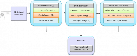
Figure 1. Overall block diagram of the proposed system
These videos received recommendations from an occupational therapist affiliated with Sri Ramachandra Medical College Research Institute (SRMC-RI). EEG signal acquisition involved the placement of Ag/AgCl electrodes on the scalp using conductive gel and tapes to improve conduction. The acquisition process followed the 10-20 International Standard, encompassing EEG signals recorded from 19 channels and two earlobes at a sampling rate of 500 Hz. Electrodes were positioned over specific cortical lobes, including the frontal (Fp1, Fp2, F3, F7, F4, F8, and Fz), temporal (T3, T5, T4, and T6), occipital (O1 and O2), parietal (P3, P4, and Pz), and central (C3, C4, and Cz) areas. Subsequently, the recorded EEG signals underwent analysis using Nihon Kohden Neurofax MEB9000 version 05-81 and software tools to apply filtering and remove artifacts. The electrode polarization was overcome by using Ag/AgCl electrodes, and powerline interference, eye movement, muscle artifacts, electrode drift, cardiac activity, and environmental noise were removed. The electroencephalogram was recorded with a sensitivity of 7 μV, with low-pass and high-pass filters applied at a cut-off frequency range of 0 to 70 Hz. The stimuli presented to the children included a video, each with duration of 60 seconds. Each participant received instructions to view five videos. The concentration level of the children with ASD during the stimuli could not be observed visually, making EEG signal acquisition necessary for better insights. The diagram is presented in Figure 1. Depicts the block diagram of the proposed system.
3.2 Feature extraction
In this section, the extraction of absolute features, delta features, and delta-delta features is described in detail.
3.2.1 Absolute features
Absolute features are defined as quantitative characteristics or measures that are directly computed from the EEG data without undergoing any additional transformation. In this work, absolute features encompass features such as LFCC, cepstral energy, and signal energy, which are extracted from the EEG data.
A. Linear Frequency Cepstral Coefficients
In essence, LFCCs are representing the spectral envelope of a signal using a set of coefficients. Due to its non-linear frequency scale, de-correlated makeup, and noise resistance, this representation is frequently utilized in signal processing [31]. Signals behave as quasi-stationary in short periods; hence a small window size should be employed while analysing LFCC features frame by frame. The inverse Fourier transform is not used as the final transform in the LFCC; instead, the Discrete Cosine Transform (DCT) is used [32]. Since the resulting coefficients are real-valued, the DCT offers an advantage over the Fourier transform in terms of ease of processing and storage. The coefficients of LFCCs are the first few DCT coefficients that describe the coarse spectral structure. The average power of the spectrum is represented by the first DCT coefficient. The broad form of the spectrum is roughly represented by the second coefficient, which is connected to the spectral centroid.
A matrix of feature vectors taken from each frame is the result of employing LFCC. In this output matrix, the columns correspond to the associated feature vector coefficients, and the rows to the corresponding frame numbers. LFCC systems in this work use only seven cepstral coefficients. Finally, the categorization method uses cepstral coefficients.
LFCC extraction from EEG using following steps:
Step 1: Framing and Windowing
The EEG signal is divided into short frames in the time domain and is quickly analyzed because it is difficult to evaluate a signal at once. The signal is split into frames that contain almost stationary signal blocks before the windowing operation is applied. Results can be improved by processing data with hamming before applying FFT.
$w(n)=0.54-0.46 \cos (2 \pi n N) \quad 0 \leq n \leq N-1$ (1)
N is the length of the window, w(n) is the window value.
Step 2: Fast Fourier Transform
To examine the various frequencies of a signal, an FFT transforms a time-domain representation of the signal into a frequency-domain representation. If a clear signal in the time domain contains cross talk, noise, or jitter, the frequency domain is excellent at revealing it. Windowing can be used to reduce the spectral leakage that results from discontinuities in the initial, non-integer number of periods of a signal. The digitizer acquires each finite sequence, and windowing decreases the amplitude of the discontinuities at the boundaries.
$X(k)=\frac{1}{N} \sum_{n=0}^{N-1} x(n) \cdot w(n) e^{-j \frac{2 \pi k n}{N}} \mathrm{n}=0,1,2, \ldots, \mathrm{N}$ (2)
x(n) is the windowed signal and N is the size of the domain.
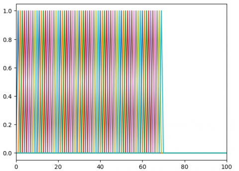
Step 3: Design an Optimized Linear Scale Filter Bank for EEG Signal
The initial filter bank will commence at position one, attain its peak at position two, and subsequently recede to zero at position three. The succeeding filter bank will start at position two, achieve its maximum at position three, reduce to zero at position four, and so on. The subsequent Eq. (3) outlines the procedure for determining these values:
$H_i(k)=\left\{\begin{array}{cc}0 & k<f_{b_i-1} \\ \frac{\left(k-f_{b_i-1}\right)}{\left(f_{b_i}-f_{b_i-1}\right)} & f_{b_i-1} \leq k \leq f_{b_i} \\ \frac{\left(f_{b_i+1}-k\right)}{f_{b_i+1}-f_{b_i}} & f_{b_i} \leq k \leq f_{b_i+1} \\ 0 & k>f_{b_i-1}\end{array}\right.$ (3)
where, the index i represents the filter number, with $f_{b_i}$ indicating the filter boundaries, which are expressed as positions determined by the sampling frequency used. Similarly, the index k pertains to the coefficients of the N-point FFT. Figure 2 depicts the linear filter bank with different frequencies.
Step 4: Log
The log energy of each filter of the linear filter bank is computed using Eq. (4)
$x_i=\ln \left(\sum_{i=0}^{N-1}|X(k)|^2 H_i(k)\right) \quad 0 \leq i \leq M$ (4)
$H_i(k)$ is the transfer function of $i^{th}$ filter.
(a)
(b)
Figure 2. Illustrate the Linear-filter bank (a) Filter bank consists of 70 filters for frequency range of 0-70 Hz (b) Filter bank consists of 22 filters for frequency range of 8 to 30Hz
Step 5: Discrete Cosine Transform
For the given frame analysis, the Cepstral representation of the EEG spectrum provides a comprehensive depiction of the signal's local spectral characteristics. Using the DCT, transform the linear spectrum coefficients (and consequently their logarithm) to a domain that resembles time, known as the quefrency domain. These features are referred to as the linear scale cepstral coefficients.
$X_k=\sum_{n=0}^{N-1} x_i \cos \left[\frac{\pi}{N}\left(n+\frac{1}{2}\right) k\right]$ (5)
B. Cepstral energy
The cepstral energy is computed by the sum of squares of the cepstral coefficients. The following equation is used to calculate the cepstral energy:
$E_C=\sum_{k=0}^{N-1}|C(k)|^2$ (6)
This type of energy is frequently employed in speech recognition systems because it offers a smoother, more reliable estimate of the energy that takes advantage of the cepstral representation of the signal [33].
C. Signal energy
The input EEG signal energy is computed by the sum of squares of the input signal [34]. The following equation is used to calculate the Signal energy:
$E=\sum_{n=0}^{N-1}|X(n)|^2$ (7)
3.2.2 Deltas and delta-deltas features
Delta features are calculated by taking the first-order difference of consecutive absolute features. They provide information about the rate of change or slope of the absolute features over time and can be useful in capturing trends or dynamics in the data.
Delta-delta features are obtained by taking the first-order difference of consecutive delta features. These features provide information about the acceleration or change in the rate of change of the absolute features and can help capture higher-order changes or patterns in the data. Both Features are utilized to analyze the temporal dynamics of a frame [35]. The following equation is used to calculate the delta coefficients:
$d_t=\frac{\sum_{n=1}^N n\left(c_{t+n}-c_{t-n}\right)}{2 \sum_{n=1}^N n^2}$ (8)
where, $d_t$ is a delta coefficient, derived from frame t and calculated using static coefficients $c_{t+n}$ to $c_{t-n}$. The usual value of N is 2. The same formula is used to produce Delta-Delta (Acceleration) coefficients, however this time; deltas are used instead of static coefficients [36].
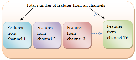
Since LFCCs frequently only include data from a single window, these cepstral coefficients are regarded as static characteristics. Calculating cepstral energy, signal energy, and first and second derivatives also referred to as delta and delta-delta derivative coefficients will provide insight into the temporal dynamics of cepstral coefficients [37]. The feature vector used in this research work has a length of 27, and it contains nine absolute features, including seven Linear Frequency Cepstral Coefficients, one cepstral energy, and one signal energy. To account for those absolute properties, nine deltas are introduced. There are added nine delta-deltas. End up with 27 features (27 features/frame ×120 frame/channel × 19 channels) for each audio-video stimuli of each ASD and TD child. Figure 3. depicts the total number of EEG features extracted.
(a)
(b)
Figure 3. Illustrates the feature extraction (a) The total number of features extracted from all channels; (b) The number of features extracted from each frame
3.3 Classifiers
The methodology consisted of two phases. In the first stage, the classification utilized the training data to build a model by establishing the correlation between the extracted features and their associated labels. Subsequently, in the second phase, the trained classification model was evaluated using new, untrained features, and the labels of the new features set were compared with the real labels to determine the accuracy of the classification algorithm. This work employed various machine learning algorithms, including KNN, MLP, SVM, Decision Tree, and ensemble classifiers such as bagging and Random forest. The particulars of the algorithms are explicated in the subsequent subsections.
3.3.1 K-Nearest neighbors
The KNN method is a supervised machine learning algorithm utilized for addressing classification and regression problems. Its approach involves classifying new data by considering the class of its k-nearest neighbors, selected using the majority voting principle. Specifically, for a given value of k, the algorithm evaluates the classes of the k closest training points to the test data point. The test data point's class is then determined depend on the majority class of the k nearest neighbors. The distance between the training and testing data points can be calculated using Euclidean, Manhattan, or Hamming distances [38]. This work utilizes Manhattan distance.
Eq. (9) for Manhattan distance is
$d(x . y)=\sum_{i=1}^n\left|x_i-y_i\right|$ (9)
where, $d(x . y)$ represents the distance between point x and point y, ∑ represent cumulative sum of n step.
The KNN algorithm is composed of several fundamental steps, as follows:
Step 1: Determine the value of k, representing the number of nearest neighbors to be examined.
Step 2: Compute the distance between the each of the training data points and new data point, utilizing a distance metric such as Euclidean distance or Manhattan distance.
Step 3: Identify the k nearest data points by selecting the ones with the smallest calculated distances.
Step 4: For classification tasks, determine the majority class among the k nearest neighbors and assign this class to the new data point.
Overall, the KNN algorithm involves a series of computations and decisions based on the value of k and the distance metric used.
3.3.2 Multi-layer perceptron
This work utilized the MLP feedforward ANN model for converting input data sets into appropriate outputs. The MLP consists of fully interconnected multiple layers, with each layer containing neurons with nonlinear activation functions, except for the input layer. One or more nonlinear hidden layers may separate the input and output layers. The error is estimated based on the labels for the initial feed-forward operation using a cost function, which is a term used to describe the error function. The cost function types include cross-entropy, mean absolute error, and mean squared error. For categorization purposes, the cross-entropy cost function is used. The weights are updated using gradient descent through backpropagation, with stochastic gradient descent being commonly employed for this optimization. In this work, the Adam optimizer is utilized for classification. After several training epochs, the model is capable of categorizing the data [39].
The activation function is defined by the following equation,
$f\left(b+\sum_i w_i x_i\right)$ (10)
where, $f()$ the activation function, b indicates the bias component, $x_i$ signifies the activation values, $w_i$ represents the weight values and b corresponds to the bias component of the model.
3.3.3 Decision tree
The decision tree algorithm is a popular machine learning technique employed for addressing both regression and classification problems. It constructs a tree-like structure to represent a set of decisions and their corresponding results. Each node in the tree like structure represents a decision based on one or more input features, while each leaf node of the tree represents the predicted output. In classification problems, the goal is to forecast the class label of a new instance based on its input features. The algorithm recursively splits the data into smaller subsets based on the input features until each subset is as homogeneous as possible concerning the target variable. At each node of the tree, the algorithm selects the feature that can best separate the data into the most homogeneous subsets using a splitting criterion, such as the Gini index, information gain, or entropy. The Gini index is employed as the splitting criterion in this work.
The formula for the Gini index is defined by Eq. (11),
$Gin \,\,i=1-\sum_{i=1}^j P(i)^2$ (11)
where, j denotes the number of classes present in the target variable, and let P(i) denote the ratio of observations that have passed in a given node, divided by the total number of observations present in that node.
Decision trees are highly regarded in machine learning due to their interpretability and ability to handle both numerical and categorical data. However, they are susceptible to overfitting, where the tree becomes too difficult and fits the training data too strictly, prominent to poor generalization performance on new data. To overcome this issue, techniques such as pruning, ensemble methods, and regularization can be applied to mitigate overfitting and enhance the performance of decision trees.
3.3.4 Support vector machine
The SVM machine learning algorithm is employed for performing both regression and classification tasks. SVM algorithm is primarily used to determine the optimal hyperplane or boundary that can effectively distinguish between different classes within the feature space. This hyperplane is selected to maximize the margin or the distance between the closest data points of each class. The margin size is indicative of the robustness and generalizability of the model for future predictions.
The equation for the hyperplane in an SVM with two classes is given by Eq. (12),
$w^T x+b=0$ (12)
where, w is the vector perpendicular to the hyper-plane, x is the input data, and b is the bias term or offset of the hyperplane from the origin. The SVM aims to identify the values of w and b that maximize the margin while ensuring that all data points are accurately classified. This is accomplished by resolving a constrained optimization problem in which the norm of w is minimized while satisfying the constraint that each data point is on the correct side of the hyperplane.
3.3.5 Ensemble learning
In disease diagnosis, an ensemble approach involves partitioning the original dataset into smaller datasets to decompose each dataset, thus enabling prediction algorithms to be applied to each decomposed dataset. By leveraging the decomposed dataset as a reference, the individual prediction outcomes are averaged to obtain an overall prediction. Allende and Valle suggest that merging models for disease diagnostic prediction can have several advantages, including the use of appropriate aggregation techniques, which can significantly improve overall diagnostic accuracy; the use of combination strategies as the optimal prediction model is often unknown; and the ability to significantly reduce errors by combining multiple predictions. Furthermore, ensembles are frequently employed for prediction for several reasons, such as improved generalizability, increased tolerance, and decreased model variance concerning data noise.
Bagging ensemble Bagging is a suitable tool for algorithms that are considered weaker or more prone to variances such as KNN or decision trees. Breiman [40] proposed the use of bagging, also known as bootstrap aggregating, as a traditional ensemble method for addressing classification issues. Bagging involves generating several samples from a single dataset using the bootstrap method with replacement, resulting in multiple trees for the same predictor variables that are combined to produce an aggregate estimate. The aggregate estimate is determined through averaging or voting for classification or regression problems, respectively [41]. The advantage of using bagging for ensemble formation is that it reduces the baseline predictor's error and can generate predictive performance estimates that are correlated with test set estimates or cross-validation [42]. However, the trees generated using bagging may lack diversity and share traits, which can limit their predictive power. To address this issue, RF was developed as a modification of the bagging method, with the addition of randomly selecting predictors at each decision tree node [43]. RF also involves choosing the optimal collection of features to describe the data [44]. Its algorithm includes the following steps: (i) generating samples from a training set using the bootstrap method with the number of observations for several predictors and variable responses; (ii) building several trees, with each node containing a subset of the number of predictor variables chosen at random; (iii) using the best subset identified in step (i) to produce a variable response estimate from each tree; and (iv) producing a final estimation by averaging the predictions acquired in step (iii). The main goal of using RF is to enhance tree performance by reducing their variance [45]. Unlike bagging, RF aims to minimize correlation among the sampled datasets by increasing randomization while developing trees. Therefore, RF outperforms bagging models by providing better predictive power due to its reduced correlation among the trees.
This section presented a comprehensive analysis of the diverse performances of multiple classifiers across distinct brain areas.
4.1 Environmental setup
Python 3.7.12 and Colab were utilized. Scikit-test Learn train split function with an 80/20 split along with many predefined models was used to divide the dataset. Normalization and standardization operations were performed using scikit-learn. The data was read and processed using Numpy, Scipy, and Pandas. The suggested model's effectiveness was evaluated through measures of accuracy, precision, specificity, sensitivity, and F1 score.
4.2 Parameter selection
Hyperparameters, which are variables that users typically specify when constructing a machine-learning model, play a crucial role in estimating the optimal parameters of the model. Before specifying the parameters, hyperparameters must be specified or utilized. One of the best features of hyperparameters is the ability to select their values. For example, k in the KNN Classifier and max depth in Random Forest Algorithms are hyperparameters. Grid Search is a method that determines the combination of hyperparameters and their values that produces the best performance out of all possible combinations. It uses that combination as its starting point and then evaluates the performance of every possible combination. Cross-validation is used together with GridSearchCV during the Grid Search process.
During the model training process, cross-validation is utilized. As a common practice, the data is separated into training sets (80%) and test sets (20%) before training the model. During cross-validation, the training dataset is further divided into training and validation data. Cross-validation with K-fold is the most widely used cross-validation method, with a k value of 10. The training data is divided into k partitions using a repetitive approach. In each iteration, k-1 partitions are used to train the model and one partition is retained for testing. The remaining partitions will be designated as test data in the following iteration, followed by the k-1 partitions as training data, and so on. In every iteration records the performance, and at the end, the average of all performances is calculated. Thus, the best hyperparameters are identified through GridSearch and cross-validation.
4.3 Model selection
Based on the literature survey, it is clear evident that both KNN and SVM demonstrate superior performance in ASD classification, while MLP and Decision Trees are also employed for this purpose. KNN is simple and it can be effective in capturing local patterns in the data. But KNN can be sensitive to the choice of k (the number of neighbors) and requires a suitable distance metric, which might not always be straightforward to define for EEG-based data. SVM is effective in handling high-dimensional feature spaces. It is robust against overfitting when the margin is properly regularized. However, SVM is sensitive to the choice of kernel function and parameters, which may require tuning for optimal performance. MLP (Multi-Layer Perceptron) can learn complex patterns and relationships in data and Decision trees provide interpretable models, allowing for transparency and insight into the decision-making process. However, MLPs and Decision trees are prone to overfitting. So it provides less accuracy when compared to KNN and SVM.
4.4 Performance analysis
In this work, Data is arranged according to classes 0 for TD and 1 for ASD for further processing and classification. While extracting the features 80% data of each class is utilized for the training of the classifier using k-fold cross-validation (k=10) and subsequently, 20% of unseen data of each class is used for the test. The classifier training was carried out using extracted features and was tested on data to forecast the label of the data and calculate the prediction accuracy for 2-classes.
4.4.1 Comparative analysis of machine learning models for all frequency bands
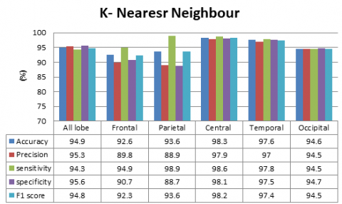
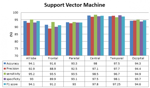
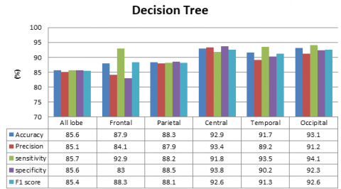
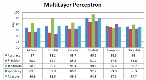
To achieve optimal classification performance, the various classifiers were employed with optimal parameter settings. The KNN classifier was specifically configured with a value of k set to 1, which enabled the classifier to assign the class label of a given test data point based on the majority voting principle. Moreover, the Manhattan distance metric was utilized for computing the distance between the training and test data points. For the Decision Tree classifier, the Gini index was utilized for binary splitting of the tree. Similarly, the MLP classifier was set to use the hyperbolic tangent (tanh) activation function and the adaptive moment estimation (adam) solver. Finally, the SVM classifier was set to use the Radial Basis Function (RBF) kernel. The performance of all the models was compared, and it was found that the KNN and SVM classifier outperformed all the other classifiers at the central lobe and temporal lobe. This is illustrated in Figure 4, which depicts the comparison of the accuracy, precision, sensitivity, specificity and F1 score of the various base models for all frequency bands.
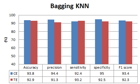
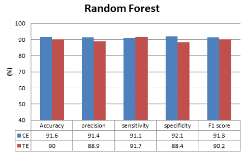
4.4.2 Comparative analysis of machine learning models for specific frequency bands
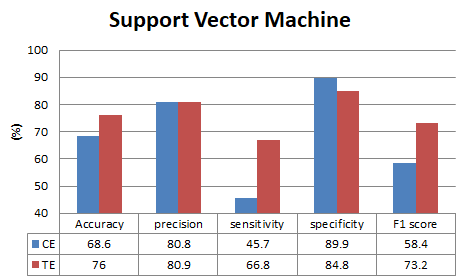
According to the analysis, KNN and SVM demonstrated higher accuracy levels at the central and temporal lobes across all frequency bands. Subsequently, SVM and KNN were utilized to evaluate the accuracy of the central and temporal lobes for specific frequency bands. Specific frequency band ranges like alpha and beta frequency bands are chosen because alpha waves appear in the electroencephalogram (EEG) when an individual is in a typical wakeful state marked by quiet restfulness, while beta EEG patterns arise when a person is alert, attentive, and actively engaged in thinking. However, the obtained accuracy was found to be minimal, prompting the adoption of the bagging ensemble method. Bagging algorithms guarantee variance reduction, overfitting avoidance, and excellent prediction stability. Random forest is an ensemble technique that aggregates the results from various models that were created using the input data to produce the final product [46]. Classification can be delayed by building many decision trees; however, studies demonstrate that using the random forest for ASD classification results in satisfactory outcomes [47]. The performance of all other models was compared, and it was found that the Baging KNN outperformed all the other classifiers at the central lobe. Figure 5. Depicts the accuracy, precision, sensitivity, specificity and F1 score of the machine learning models for specific frequency bands. Table 1 displays a comparison between our proposed approach's accuracy and that of an existing method.
(a)
(b)
(c)
(d)
Figure 4. Comparative analysis of various base model techniques for all frequency bands (a) KNN, (b) SVM, (c) Decision Tree, and (d) MLP
Table 1. Comparison between our proposed approach and an existing method
|
Sources |
Features and Methods |
Classifiers |
Accuracy(%) |
|
Igberaese et al. [21] |
Power Spectral Density (PSD) |
KNN |
89.2 |
|
Abdolzadegan et al. [22] |
Fast Fourier Transform (FFT), Wavelet Transform, Power Spectrum, Entropy, Lyapunov Exponent, Correlation Dimension, Fractal Dimension, Synchronization Likelihood, and Detrended Fluctuation Analysis. Minimum-Redundancy Maximum Relevancy (mRmR), Genetic Algorithm (GA), Mutual Information (MI), and Information Gain (IG) |
SVM |
90.5 |
|
Sinha et al. [23] |
Alpha, beta, delta, theta, and gamma, kurtosis, skewness, mean, standard deviation, variance, and Shannon entropy |
Subspace KNN |
92.8 |
|
Ibrahim et al. [24] |
DWT, Shannon entropy |
KNN |
94.6 |
|
Jamal et al. [ 28] |
Network measures, synchrostates, |
SVM (Second Order Polynomial Kernel) |
94.7 |
|
Tawhid et al. [25] |
Short-Time Fourier Transform, Principal Component Analysis |
SVM |
95.25 |
|
RoopaRechal et al. [26] |
Variational Mode Decomposition and RELIEFF |
SVM |
95.4 |
|
Alotaibi and Maharatna [29] |
Trial-averaged Phase-Locking Value (PLV) approach |
Cubic SVM |
95.8 |
|
Baygin et al. [27] |
One dimensional local binary pattern (1D-LBP), Short Time Fourier Transform (STFT), deep features from MobileNet, SqueezeNet, shuffleNet and RELIEFF |
SVM |
96.44 |
|
Proposed method |
LFCC, cepstral energy, signal energy and their delta and their delta-delta derivatives |
KNN |
98.3 |
(a)
(b)
(c)
(d)
Figure 5. Comparison of machine learnig models for specific frequency band. (a) KNN, (b)SVM, (c)Bagging KNN, and (d) Random Forest
Researchers from all over the world are currently tackling the issue of objective identification to differentiate between ASD and TD. The challenge comes from the vast range of symptoms among children with ASD; some may have good social abilities but struggle with communication, whereas others may have language skills but struggle with social interaction. The fact that ASD symptoms may not become obvious until later in childhood or maybe adulthood further complicates the problem of differentiating between TD and ASD in young children. To address this issue, the LFCC, cepstral energy, and signal energy of the EEG signal were studied. Combining delta and delta-delta derivative features with absolute features to capture rapid changes in the EEG signal increased the accuracy of ASD and TD categorization. The findings of this study demonstrate that by combining LFCC, cepstral energy, signal energy, and their delta and delta-delta derivatives, the KNN method can reach the greatest classification accuracy of 98.3% for all frequency bands in EEG at the central lobe. To reduce computation time, the experiment focused on identifying which lobe provided greater discrimination between ASD and TD. The central and temporal lobes collaborated to provide accuracy above 97% across all frequency bands in EEG. Extrapolating LFCC for particular frequency bands, such as the alpha and beta frequency bands in the central and temporal lobes, allowed for additional study because KNN and SVM classifiers provided greater accuracy in assessments of all frequency bands. The accuracy of the SVM classifier was 68% for the central lobe and 76% for the temporal lobe, respectively. The central lobe reached the highest accuracy of 93.8% by employing bagging KNN to boost accuracy even further.
This work developed two distinct linear scale filterbanks. The first filter bank aims to extract all frequency bands that exist in EEG signals, while the second filter bank is specifically designed to extract alpha and beta frequency bands. The proposed methodology is utilized to identify the optimal number of electrodes required for the acquisition of EEG signals, which can effectively differentiate individuals with ASD from those who are TD. One limitation of the study is that it focuses solely on extracting spectral envelope details using LFCC to obtain more discriminating brain lobe regions. In future studies, it is recommended to incorporate features from the time-frequency domain, time domain, and frequency domain to extract a broader range of information on the brain dynamics of EEG signals, thereby providing a comprehensive characterization of the EEG signal.
[1] Kanner, L. (1968). Autistic disturbances of affective contact. Acta Paedopsychiatrica, 35(4): 100-136.
[2] Asperger, H. (1991). Autistic Psychopathy. In Childhood; Frith, U., Series Ed., Autism and Asperger syndrome; Cambridge University Press: New York, NY, US, p 92. https://doi.org/10.1017/CBO9780511526770.002
[3] Zeidan, J., Fombonne, E., Scorah, J., Ibrahim, A., Durkin, M. S., Saxena, S., Yusuf, A., Shih, A., Elsabbagh, M. (2022). Global prevalence of autism: A systematic review update. Autism Research, 15(5): 778-790. https://doi.org/10.1002/aur.2696
[4] Maenner, M.J., Shaw, K.A., Baio, J., Washington, A., Patrick, M., DiRienzo, M., Christensen, D.L., Wiggins, L.D., Pettygrove, S., Andrews, J.G., Lopez, M., Hudson, A., Baroud, T., Schwenk, Y., White, T., Rosenberg, C.R., Lee, L.C., Harrington, R.A., Huston, M., Hewitt, A., Esler, A., Hall-Lande, J., Poynter, J.N., Hallas-Muchow, L., Constantino, J.N., Fitzgerald, R.T., Zahorodny, W., Shenouda, J., Daniels, J.L., Warren, Z., Vehorn, A., Salinas, A., Durkin, M.S., Dietz, P.M. (2020). Prevalence of autism spectrum disorder among children aged 8 years — Autism and developmental disabilities monitoring network, 11 sites, United States, 2016. MMWR Surveill Summ, 69(4): 1-12. https://doi.org/10.15585/mmwr.ss6904a1
[5] Canada, P. H. A. of. Autism Spectrum Disorder among Children and Youth in Canada 2018. https://www.canada.ca/en/public-health/services/publications/diseases-conditions/autism-spectrum- disorder-children-youth-canada-2018.html, accessed on 2022, April 28.
[6] Sato, W., Uono, S. (2019). The atypical social brain network in Autism: Advances in structural and functional MRI studies. Current Opinion in Neurology, 32(4): 617-621. https://doi.org/10.1097/WCO.0000000000000713
[7] Radhakrishnan, M., Boruah, S., Ramamurthy, K. (2022). EEG-based anamoly detection for autistic kids-A pilot study. Traitement du Signal, 39(3): 1005-1012. https://doi.org/10.18280/ts.390327
[8] Menaka, R., Karthik, R., Parthasarathy, A., Manideep, P., Varsha, V. (2022). Coherence analysis in the brain network of ASD children using connectivity model and graph theory. Journal of Scientific & Industrial Research, 81(9): 940-951. https://doi.org/10.56042/jsir.v81i09.52350
[9] Radhakrishnan, M., Ramamurthy, K., Kothandaraman, A., Madaan, G. and Machavaram, H. (2021). Investigating EEG signals of autistic individuals using detrended fluctuation analysis. Traitement du Signal, 38(5): 1515-1520. https://doi.org/10.18280/ts.380528
[10] Sheikhani, A., Behnam, H., Mohammadi, M.R., Noroozian, M., Golabi, P. (2008). Connectivity analysis of quantitative electroencephalogram background activity in autism disorders with short time fourier transform and coherence values. In 2008 Congress on Image and Signal Processing, pp 207-212. https://doi.org/10.1109/CISP.2008.595
[11] Ayvaz, U., Gürüler, H., Khan, F., Ahmed, N., Whangbo, T., Akmalbek Bobomirzaevich, A. (2022). Automatic speaker recognition using mel-frequency cepstral coefficients through machine learning. Computers, Materials & Continua, 71(3): 5511-5521. https://doi.org/10.32604/cmc.2022.023278
[12] Wang, Y., Lawlor, B. (2017). Speaker recognition based on MFCC and BP neural networks. In 2017 28th Irish Signals and Systems Conference (ISSC), Killarney, Ireland, pp 1-4. https://doi.org/10.1109/ISSC.2017.7983644
[13] Mangalam, A.R., Singh, S., Lalremtluanga, C., Kumar, P., Das, R., Basu, J., Chatterjee, S. (2022). Emotion recognition from mizo speech: A signal processing approach. In 2022 IEEE International Conference on Distributed Computing and Electrical Circuits and Electronics (ICDCECE), Ballari, India, pp 1-6. https://doi.org/10.1109/ICDCECE53908.2022.9793078
[14] Kamarulafizam, I., Salleh, S., Najeb, S.J.M., Ariff, A.K., Chowdhury, A. (2007). Heart sound analysis using MFCC and time frequency distribution. In World Congress on Medical Physics and Biomedical Engineering 2006; Magjarevic, R., Nagel, J. H., Eds.; IFMBE Proceedings; Springer: Berlin, Heidelberg, pp 946–949. https://doi.org/10.1007/978-3-540-36841-0_225
[15] Muda, L., Begam, M., Elamvazuthi, I. (2010). Voice recognition algorithms using Mel Frequency Cepstral Coefficient (MFCC) and Dynamic Time Warping (DTW) techniques. https://doi.org/10.48550/arXiv.1003.4083
[16] Murty, K.S.R., Yegnanarayana, B. (2006). Combining evidence from residual phase and MFCC features for speaker recognition. IEEE Signal Processing Letters, 13(1): 52-55. https://doi.org/10.1109/LSP.2005.860538
[17] Zubair, K. M.; Mashkur, B. S.; Nor, N.M. (2022). Early detection on autistic children by using EEG signals. International Journal on Perceptive and Cognitive Computing, 8(1): 59-64.
[18] Jagtap, S.S., Kadbe, P.K., Arotale, P.N. (2016). System propose for Be acquainted with newborn cry emotion using linear frequency cepstral coefficient. In 2016 International Conference on Electrical, Electronics, and Optimization Techniques (ICEEOT), Chennai, India, pp. 238-242. https://doi.org/10.1109/ICEEOT.2016.7755094
[19] Menaka, R., Karthik, R., Saranya, S., Niranjan, M., Kabilan, S. (2023). An improved alexnet model and cepstral coefficient-based classification of autism using EEG. Clinical EEG and Neuroscience. https://doi.org/10.1177/15500594231178274
[20] Golmohammadi, M., Harati Nejad Torbati, A.H., Lopez de Diego, S., Obeid, I., Picone, J. (2019). Automatic analysis of EEGs using big data and hybrid deep learning architectures. Frontiers in Human Neuroscience, 13: 76. https://doi.org/10.3389/fnhum.2019.00076
[21] Igberaese, A.E., Tcheslavski, G.V. (2018). EEG power spectrum as a biomarker of autism: A pilot study. International Journal of Electronic Healthcare, 10(4): 275-286. https://doi.org/10.1504/IJEH.2018.101446.15
[22] Abdolzadegan, D., Moattar, M.H., Ghoshuni, M. (2020). A robust method for early diagnosis of autism spectrum disorder from EEG signals based on feature selection and DBSCAN method. Biocybernetics and Biomedical Engineering, 40(1): 482-493. https://doi.org/10.1016/j.bbe.2020.01.008
[23] Sinha, T., Munot, M.V., Sreemathy, R. (2022). An efficient approach for detection of autism spectrum disorder using electroencephalography signal. IETE Journal of Research, 68(2): 824-832. https://doi.org/10.1080/03772063.2019.1622462
[24] Ibrahim, S., Djemal, R., Alsuwailem, A. (2018). Electroencephalography (EEG) signal processing for epilepsy and autism spectrum disorder diagnosis. Biocybernetics and Biomedical Engineering, 38(1): 16-26. https://doi.org/10.1016/j.bbe.2017.08.006
[25] Tawhid, M.N.A., Siuly, S., Wang, H. (2020). Diagnosis of autism spectrum disorder from EEG using a time–Frequency spectrogram image-based approach. Electronics Letters, 56(25): 1372-1375. https://doi.org/10.1049/el.2020.2646
[26] Roopa Rechal, T., Rajesh Kumar, P. (2021). Computer aided diagnosis of ASD based on EEG using RELIEFF and supervised learning algorithm. Turkish Journal of Computer and Mathematics Education (TURCOMAT), 12(6): 253-260. https://doi.org/10.17762/turcomat.v12i6.1362
[27] Baygin, M., Dogan, S., Tuncer, T., Datta Barua, P., Faust, O., Arunkumar, N., Abdulhay, E.W., Emma Palmer, E., Rajendra Acharya, U. (2021). Automated ASD detection using hybrid deep lightweight features extracted from EEG signals. Computers in Biology and Medicine, 134: 104548. https://doi.org/10.1016/j.compbiomed.2021.104548
[28] Jamal, W., Das, S., Oprescu, I.A., Maharatna, K., Apicella, F., Sicca, F. (2014). Classification of autism spectrum disorder using supervised learning of brain connectivity measures extracted from synchrostates. Journal of Neural Engineering, 11(4): 046019. https://doi.org/10.1088/1741-2560/11/4/046019
[29] Alotaibi, N., Maharatna, K. (2021). Classification of autism spectrum disorder from EEG-based functional brain connectivity analysis. Neural Computation, 33: 1914-1941. https://doi.org/10.1162 /neco_a_01394
[30] Mohanta, A., Mukherjee, P., Mirtal, V.K. (2020). Acoustic features characterization of autism speech for automated detection and classification. In 2020 National Conference on Communications (NCC), pp 1-6. https://doi.org/10.1109/NCC48643.2020.9056025
[31] D, G.R. (2016). Analysis of MFCC features for EEG signal classification. International Journal of Advances in Signal and Image Sciences, 2(2): 14-20. https://doi.org/10.29284/ijasis.2.2.2016.14-20
[32] Chenchah, F., Lachiri, Z. (2015). Acoustic emotion recognition using linear and nonlinear cepstral coefficients. International Journal of Advanced Computer Science and Applications (IJACSA), 6(11): 135-138. http://dx.doi.org/10.14569/IJACSA.2015.061119
[33] Harati, A., Golmohammadi, M., Lopez, S., Obeid, I., Picone, J. (2015). Improved EEG event classification using differential energy. In 2015 IEEE Signal Processing in Medicine and Biology Symposium (SPMB), Philadelphia, PA, USA, pp 1-4. https://doi.org/10.1109/SPMB.2015.7405421
[34] Hsu, Y.L., Yang, Y.T., Wang, J.S., Hsu, C.Y. (2013). Automatic sleep stage recurrent neural classifier using energy features of EEG signals. Neurocomputing, 104: 105-114. https://doi.org/10.1016/j.neucom.2012.11.003
[35] Musaev, M., Abdullaeva, M., Ochilov, M. (2022). Advanced feature extraction method for speaker identification using a classification algorithm. AIP Conference Proceedings, 2656(1): 020022. https://doi.org/10.1063/5.0106614
[36] Armitage, R. (1995). The distribution of EEG frequencies in REM and NREM sleep stages in healthy young adults. Sleep, 18(5): 334-341. https://doi.org/10.1093/sleep/18.5.334
[37] Khalilzad, Z., Kheddache, Y., Tadj, C. (2022). An entropy-based architecture for detection of sepsis in newborn cry diagnostic systems. Entropy, 24(9): 1194. https://doi.org/10.3390/e24091194
[38] Jagadeeswara Rao, G., Siva Prasad, A., Sai Srinivas, S., Sivaparvathi, K., Panda, N. (2022). Data classification by ensemble methods in machine learning. In Advances in Intelligent Computing and Communication; Mohanty, M. N., Das, S., Eds.; Lecture Notes in Networks and Systems; Springer Nature: Singapore, pp 127-135. https://doi.org/10.1007/978-981-19-0825-5
[39] Alnuaim, A.A., Zakariah, M., Shukla, P.K., Alhadlaq, A., Hatamleh, W.A., Tarazi, H., Sureshbabu, R., Ratna, R. (2022). Human-computer interaction for recognizing speech emotions using multilayer perceptron classifier. Journal of Healthcare Engineering, 2022: 6005446. https://doi.org/10.1155/2022/6005446
[40] Breiman, L. (1996). Bagging predictors. Machine Learning, 24(2): 123-140. https://doi.org/10.1007/BF00058655
[41] Erdal, H., Karahanoğlu, İ. (2016) Bagging ensemble models for bank profitability: An emprical research on turkish development and investment banks. Applied Soft Computing, 49: 861-867. https://doi.org/10.1016/j.asoc.2016.09.010
[42] Hamze-Ziabari, S.M., Bakhshpoori, T. (2018). Improving the prediction of ground motion parameters based on an efficient bagging ensemble model of M5 and CART algorithms. Applied Soft Computing, 68: 147-161. https://doi.org/10.1016/j.asoc.2018.03.052
[43] Breiman, L. (2001). Random forests. Machine Learning, 45(1): 5-32. https://doi.org/10.1023/A:1010933404324
[44] Thakur, M., Kumar, D. (2018). A hybrid financial trading support system using multi-category classifiers and random forest. Applied Soft Computing, 67: 337-349. https://doi.org/10.1016/j.asoc.2018.03.006
[45] He, H., Zhang, W., Zhang, S. (2018). A novel ensemble method for credit scoring: Adaption of different imbalance ratios. Expert Systems with Applications, 98: 105-117. https://doi.org/10.1016/j.eswa.2018.01.012
[46] Liaw, A., Wiener, M. (2002). Classification and regression by randomForest. R News, 2(3): 18-22.
[47] Grossi, E., Olivieri, C., Buscema, M. (2017). Diagnosis of autism through EEG processed by advanced computational algorithms: A pilot study. Computer Methods and Programs in Biomedicine, 142: 73-79. https://doi.org/10.1016/j.cmpb.2017.02.002