Chander Prabha![]() | Sukhvinder Kaur
| Sukhvinder Kaur![]() | Meena Malik
| Meena Malik![]() | Mueen Uddin
| Mueen Uddin![]() | Durgesh Nandan*
| Durgesh Nandan*![]()
© 2023 IIETA. This article is published by IIETA and is licensed under the CC BY 4.0 license (http://creativecommons.org/licenses/by/4.0/).
OPEN ACCESS
Automatic Speaker Recognition (ASR) is a crucial application in the realm of speech processing, with Artificial Intelligence (AI) being extensively employed in areas such as authentication, surveillance, forensics, and security. The cornerstone processes of these applications encompass feature matching, feature extraction, and performance evaluation. However, the present speaker identification and verification techniques are not without their flaws, including vulnerability to distortion resulting from noise and the ability to mimic signals via voice recording devices. Given these challenges, there's a pressing need for a fresh feature extraction technique that offers robust speaker identification using an enhanced spectrogram. This paper addresses this need by proposing an innovative and efficient feature extraction methodology, christened "Optimized Variance Spectral Flux (OVSF)". This potent technique, based on the Daubechies 40 wavelet and power spectrum of a signal, facilitates the extraction of unique features of the speaker. For the feature matching phase in speaker recognition, the characteristics of different speakers are compared by applying the time-honored Bayesian information criterion distance metric. The proposed system's effectiveness is assessed through a series of metrics including Receiver Operating Characteristics (ROC), detection error trade-off curves, the Equal Error Rate (EER), and the Area under the Curve (AUC). The experimental results yield an AUC and EER for the proposed method of 94.38 and 10.3564, respectively, indicating a higher accuracy than the mel-frequency cepstral coefficient technique.
Daubechies wavelet, Bayesian information criterion, optimized variance spectral flux, mel-frequency cepstral coefficients
The application of voice-based speaker recognition in the arenas of forensics, biometrics, voice call centres, voice search, and diverse security applications (inclusive of banking access, computer access control, and telephonic transactions) has been the subject of heightened interest. This attention is not without substantial financial implications, driven in part by the utilisation of audio recording devices in criminal documentation and the burgeoning use of mobile technologies in thwarting crime and nefarious activities, notably international terrorism.
In the forensic sphere, Automatic Speaker Recognition (ASR) has demonstrated its capacity to yield accurate and reliable results within controlled environments, given adequate signal quality and sufficient speech duration. However, the informative richness of the voice signal, encapsulating details about the speaker, the language used, the duration of speech, the speaker's emotional state, and the environmental context, introduces a myriad of challenges.
Conventional speaker recognition methods, characterized by their labor-intensive nature, necessitate considerable efforts and time for the pre-processing of audio recordings. As such, the strategic utilisation of feature extraction methods in automated speaker recognition could significantly streamline the data processing workflow, thereby enhancing performance efficiency [1].
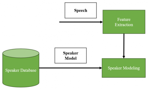
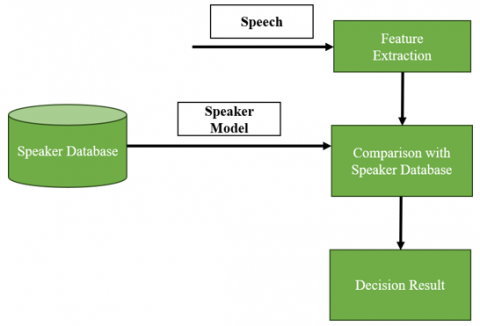
The ASR system is structured around two core modules: the enrolment phase (Figure 1), and the recognition phase, which subsumes identification or verification procedures (Figure 2). Feature vectors are derived from raw signals in the feature extraction module during transformation. This phase is crucial, as it preserves speaker-specific characteristics (such as frequency, loudness, and pitch time) while curtailing the statistical redundancies of the raw signal through the use of feature vectors in the training phase. During the recognition phase, a similarity score, or recognition rate, is obtained from the voices of unidentifiable individuals and compared to the models housed in the system database. The final decision is rendered based on this similarity score.
Prior research has contributed to the understanding and development of speaker recognition systems. Chaudhary et al. [2] conducted a comparative analysis of speech features in audio recordings for speaker identification systems. A comprehensive review of speaker recognition, encompassing its past, present, and future, was published in 2021 [3]. Earlier, in 2009, a study delineated the various disciplines of speech processing, highlighting the uses and limitations of speech recognition, segmentation, and diarization [4]. Thanks to these and other efforts, Speaker Recognition Systems (SRS) and speech performance have seen remarkable improvements over the years, with noise reduction and speech signal enhancement playing a significant role [5].
Figure 1. Enrollment phase
Figure 2. Recognition phase
In 2010, Kinnunen and his colleagues ventured into the exploration of super vectors as features in text-independent Speaker Recognition Systems [6]. Lee et al. [7] later proposed optimised features for speaker recognition, aiming to enhance performance and minimise potential degradation. With the advent of deep learning techniques, a new horizon was opened in speaker recognition, as outlined in the study [8]. The application of Mel Frequency Cepstral Coefficients (MFCCs) for tasks concerning speaker recognition has been described in the study [9]. However, current speaker verification techniques face challenges related to signal impersonation via voice recording devices. Wavelets, particularly high-level features, provide a promising solution. Not only do they help improve accuracy, but they also enhance effectiveness, given their resistance to channel effects. In 2017, a novel feature-matching technique was proposed that leveraged a T-test distance metric with an enhanced spectrogram based on Daubechies wavelet. This technique was designed for robust speaker identification and yielded superior results. However, its complexity led to slower response times [10]. Thus, despite advancements, the field continues to grapple with the delicate balance between accuracy and efficiency, presenting an ongoing area for exploration and innovation.
1.1 Objectives
The overarching goal of this study is to circumvent the limitations and challenges inherent in existing speaker recognition system algorithms and to introduce an improved, simple, efficient, and rapid novel approach. The development of this novel method is predicated on the accomplishment of the following tasks:
1.2 Contribution
The seminal contribution of this paper is the development of a novel feature extraction technique, OVSF, for an ASR. This technique leverages the Daubechies 40 wavelet and Variance Spectral Flux (VSF) to extract unique speech features of an individual. The refined and enhanced features derived from this method diverge from those obtained in previous studies, demonstrating promising performance when implemented in ASR.
1.3 Structure
This paper initiates with an overview of the ASR, followed by a definition of the study objectives and its contribution. Section 2 delves into the proposed feature extraction technique, which harnesses the power of VSF and Discrete Wavelet Transform (DWT), with the Bayesian Information Criterion (BIC) deployed for feature matching within feature classification. Section 3 elucidates the proposed speaker recognition model and outlines its performance evaluation criteria, encompassing the ROC, the AUC, DET curves, and the EER. Experimental results, which illustrate the recognition tests, are presented and discussed in Section 4. Based on these findings, final remarks and conclusions are drawn in Section 5.
2.1 Feature extraction techniques
The objective of feature extraction is to lessen transmission bandwidth, power, and data (in terms of memory space) by capturing the speaker’s essential characteristics. It is also required to enhance weak speech signals and measure the variability of the spectrum of speech signals over time for different speakers. The Spectral Flux (SF) is a useful measure for distinguishing signals whose spectrum changes slowly from those whose spectrum changes quickly [11]. The Wavelet Transform (WT) has excellent multi-resolution properties of time, frequency, and amplitude, and therefore it is used for extracting the localised contributions of the signal of interest. It also has the property to enhance the signal and suppress the noise from the speech signal [12, 13]. So, in this research work, two algorithms, WT and SF, are combined and a new technique, OVSF, is proposed to extract optimised features for speaker identification and verification. This paper employs one more existing feature extraction method, which is based on DWT-MFCC, for comparison with the proposed technique. The detailed descriptions with graphical outputs of DWT, MFCC, and OVSF are illustrated in the following section.
2.1.1 Discrete wavelet transform
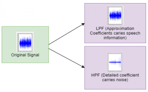
Since the 1990s, to solve engineering problems, DWT has been extensively used due to its time resolution property and high frequency [14]. In the time-frequency domain, it can examine a signal simultaneously. It also improves speech signal strength by denoising [15]. The signal (speech) is broken into subsequent high- and low-frequency component levels throughout the wavelet transformation process [16]. Figure 3 depicts that when DWT is applied to the signal (speech), it is split into two equal parts. The first part is the low-frequency noise-free speech (i.e., approximation coefficients), which carries about 98% of its information with scaled amplitude. The second part is a high-frequency signal (i.e., detail coefficient) representing noise.
Figure 3. Decomposition of the speech signal into “approximations” and “details” Using DWT
The WT has described the product of the mother wavelet ψ(t) and an input signal x(t). It is represented in Eq. (1).
$\mathrm{W}_\psi \mathrm{x}(\mathrm{m}, \mathrm{n})=\frac{1}{\sqrt{\mathrm{m}}} \int_{\infty}^{-\infty} \mathrm{x}(\mathrm{t}) \psi *\left(\frac{\mathrm{t}-\mathrm{n}}{\mathrm{m}}\right) \mathrm{dt}$ (1)
In Eq. (1), mother wavelet is:
$\Psi_{m, n}(t)=\psi\left(\frac{t-n}{m}\right)$ (2)
where, m is scale parameter and n is shift parameter. The DWT function (at time location tN and level N) can be expressed as in Eq. (3):
$\mathrm{D}_{\mathrm{N}}\left(\mathrm{t}_{\mathrm{N}}\right)=\mathrm{x}(\mathrm{t}) \psi_{\mathrm{m}}\left(\frac{\mathrm{t}-\mathrm{t}_{\mathrm{N}}}{2^{\mathrm{N}}}\right)$ (3)
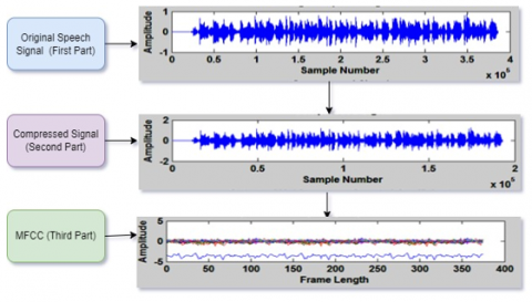
where, N is the decomposition filter that scales the output by a factor of 2N (at frequency level N). Eq. (3) of DWT is applied to compress and scale the original speech signal, as shown in Figure 4. This figure has three parts. The first part is the original speech waveform, which has 385718 samples. When DWT is applied, the number of samples is reduced to 192862, which is graphically represented in the second part of Figure 4. Further, the compressed signal goes through the feature extraction methods MFCC and OVSF.
Figure 4. Original speech signal, compressed speech signal, and its MFCC
2.1.2 Mel frequency cepstral coefficient
For reducing data size, feature extraction is considered the most significant part of speech processing. MFCC is a common technique for extracting speech signal features from the SIS. In a noisy environment, its performance degrades. The term mel is derived from a clipping of the word melody, and it is a unit of pitch. The alliance between the mel and the linear frequency scale is described in the study [17] and expressed as fmel = 2595log(1 + f/700).
To obtain the MFCC features of the preprocessed signal using Daubechies 40 wavelet, the cepstral magnitude of FFT frequency bins (i.e., based on a human auditory perception model) is averaged within frequency bands spaced like a mel scale [18]. It is estimated by applying the following steps [9]:
i. Apply Discrete Fourier Transform (DFT) on the windowed signal.
$\mathrm{h}(\mathrm{n})=\left\{\begin{array}{c}1, \quad 0 \leq \mathrm{n} \leq \mathrm{N}-1 \\ 0, \text { else }\end{array}\right\}$ (4)
$X(K)=\sum_{n=0}^{N-1} x(n) e^{-j 2 n K / N},(0 \leq n, K \leq N-1)$ (5)
ii. The power spectrum of $X(K)$ is estimated as $\left|\mathrm{X}(\mathrm{K})^2\right|$ and then converted into mel scale using filter bank $\left(\mathrm{H}_{\mathrm{M}}(\mathrm{K})\right)$ as follows:
$\sum\left|\mathrm{X}(\mathrm{K})^2\right| \mathrm{H}_{\mathrm{M}}(\mathrm{K}),(0 \leq \mathrm{m} \leq \mathrm{M})$ (6)
iii. Next step is to compute logarithm of frequency band energy obtained from Eq. (6).
$\mathrm{L}_{\mathrm{M}}=\ln \sum\left|\mathrm{X}(\mathrm{K})^2\right| \mathrm{H}_{\mathrm{M}}(\mathrm{K}),(0 \leq \mathrm{m} \leq \mathrm{M})$ (7)
iv. Finally, the frequency information obtained in Eq. (7) is compressed by taking its Discrete Cosine Transform (DCT), and then the first 10 MFCC coefficients are selected as the best unique features.
v. $c(n)=\sum L_M \cos \left(\frac{\pi n\left(m+\frac{1}{2}\right)}{M}\right)$ (8)
Graphically, the MFCC of the speech signal is revealed in the last waveform of Figure 4. The Voice waveform of a text message is seen in Figure 5.
Figure 5. Steps to extract VSF of speech signal [11]
To design a database for training and testing purposes, we used the Audacity tool (http://audacity.sourceforge.net) to record twenty candidates' voices. The voice part provides ten varieties of the varied physical voice of the standard spoken text. Speech's spectral palette can be viewed as the MFCC spectrum.
2.1.3 Proposed feature extraction technique (OVSF) based on variance spectral flux (VSF) and DWT
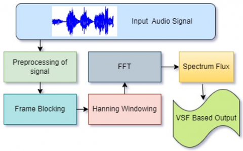
VSF is a powerful feature extraction technique usually used to segment speech and non-speech signals in an audio recording. It is based on the signal’s power spectrum. The features of speech using VSF are obtained by following the steps shown in Figure 5.
The audio signal is pre-processed to remove DC components, and then it is normalised. It is not practical to consider the whole input signal at once, as it is fundamentally non-stationary in nature. So, the normalised input signal is transformed into a piecewise stationary ordering of ‘frames’ of length 20–30 milliseconds.
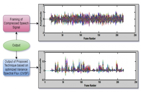
Figure 6. Outputs of framing of the compressed speech signal and proposed technique based on OVSF
A window function, such as a Henning window, typically multiplies the frames to help with edge effects during spectral analysis. After each frame has been processed, the window has shifted from the start time to the next frame by a frame shift that is an amount of time less than the length of a frame (typically 10 ms), as shown in the first part (framing of the compressed speech signal) of Figure 6.
It is further converted into a frequency domain by using FFT. The most important step of VSF is the estimation of Spectral Flux (SF). When the input signal is changing, the SF is a measure of the variation in the input signal’s power spectrum. The SF is computed by comparing one frame against the previous frame on the basis of the power spectrum. Between the two normalised spectrum magnitudes, it is an ordinary Euclidean norm and is defined as in Eq. (9) as follows:
$\mathrm{SF}=\left\|\mathrm{S}_{\mathrm{i}}-\mathrm{S}_{\mathrm{i}-1}\right\|_2=\frac{1}{\mathrm{~N}}\left(\sum_{\mathrm{k}=0}^{\mathrm{N}-1}\left(\mathrm{~S}_{\mathrm{i}}(\mathrm{k})-\mathrm{S}_{\mathrm{i}-1}(\mathrm{k})\right)^2\right)^{\frac{1}{2}}$ (9)
where, $S_i$ represents the frames spectrum magnitude vector and is given in Eq. (10).
$\left.\mathrm{S}_{\mathrm{i}}(\mathrm{k})=\mid \sum_{\mathrm{n}=0}^{\mathrm{N}-1} \mathrm{~s}\left(\mathrm{n}+\frac{\mathrm{N}_{\mathrm{i}}}{2}\right) \omega(\mathrm{n}) \exp \frac{-2 \pi \mathrm{kn}}{\mathrm{N}}\right\} \mid \mathrm{k} \in[0, \mathrm{~N}-1]$ (10)
where, $s\left(n+\frac{N_i}{2}\right)$ is audio data, $\omega(n)$ is the window function and N is the window size. A Hanning window is used in this case [19].
The proposed feature extraction technique in this research “OVSF” is based on DWT and VSF. Therefore, Eq. (10) is applied to the frames of approximation coefficients obtained from DWT. The speech signal detects the variance in its frequency, as shown in the bottom part (proposed technique based on OVSF) of Figure 6.
2.2 Feature matching technique
Many distance metrics and speaker classification algorithms have been proposed for speaker identification [17, 19]. Popular distance metrics are Bayesian Information Criteria (BIC), Generalised Likelihood Ratio (GLR), and Cross Likelihood Ratio (CLR). The BIC is probably the most extensively used metric of these three due to its effectiveness and simplicity [20].
2.2.1 Bayesian information criterion for speaker classification
In this paper, the proposed speaker recognition method uses the delta BIC distance metric to find the distance between the features of two speakers. Zero distance between two speakers shows similar speakers. Two speakers, i and j, of frame lengths Ni and Nj and parameterized acoustic feature vectors of Xi and Xj are considered, respectively. Their respective standard deviation and mean values are µj, ơj and µi, ơi. On fusing speaker’s Xi and Xj into X, their variance and mean turned as ơ and µ respectively, with length N of frame. Then the estimation of distance between the two speakers is in Eq. (11) as:
$\Delta \mathrm{BIC}=\frac{\mathrm{N}}{2} \log \left|\sum \mathrm{X}\right|-\frac{\mathrm{Ni}}{2} \log \left|\sum \mathrm{Xi}\right|-\frac{\mathrm{N} \mathrm{j}}{2} \log \left|\sum \mathrm{X} j\right|-\lambda \mathrm{P}$ (11)
where, λ is a free design parameter. Its value is 10 and it depends on the data being modelled.
P is a function of the number of free parameters in the model and is known as penalty term as presented in Eq. (12) as:
$P=\frac{1}{2}\left(d+\frac{1}{2} d(d+1)\right)$ (12)
The similarity of the two speakers depends on the value of delta BIC. It should be low for similar speakers.
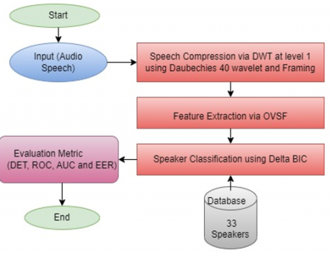
A novel feature extraction technique based on DWT and VSF is proposed in this research work, as explained in the previous section. This section elucidates the implementation of the proposed method in the speaker recognition system with the help of a diagram, as shown in Figure 7.
It follows the same procedure as a conventional recognition system (i.e., feature extraction and feature matching), but with some modifications. Based on the DWT, the audio signals were first enhanced and compressed in the ratio of 1:2 at level 1. It is done by using the Daubechies 40 (db40) wavelet with an energy of 99.9% (approx.). Next, the features of the compressed signal were detected using the proposed method (VSF). After that, the distance metric delta BIC is applied to its output for feature matching and speaker classification.
Figure 7. Proposed diagram of a speaker recognition system
This research work is divided into two parts: SR using the proposed OVSF method and SR using the traditional MFCC.
The algorithm for its implementation follows the following steps:
Step 1: Input data
Input the audio recordings of 33 speakers in.wav form. A graphic representation of the waveform of the first speaker is shown in part of Figure 5. On each recording, the following steps are applied in sequence and saved.
Step 2: Feature Extraction
Step 3: Feature Matching
All the extracted features of 33 speakers are arranged in a [33×33] matrix for feature matching using the distance metric algorithm BIC, and then the obtained result is converted into a single column. The obtained results are the hypothesised results.
Step 4: Performance Evaluation
Hypothesised results and ground truth are compared according to the confusion matrix given in Table 1 and plotted as ROC and DET to compute area under the curve and equal error rate.
Step 5
Step numbers 1 to 4 are repeated by using the traditional algorithm MFCC for feature extraction instead of OVFS.
Step 6
Finally, performance results obtained from both systems using DET [21], ROC [22, 23], AUC, and EER are compared.
The evaluation process results in four possible outcomes, as shown in Table 1, to check the existence of a given speaker in the specified database. Hit (Ground truth says the speaker is present in the database and the predicted value is “Present''), miss (Ground truth says the speaker is present in the database and the predicted value is “Absent''), false alarm (Ground truth says the speaker is absent in the database and the predicted value is “Present"), and correct rejection (Ground truth says the speaker is absent in the database and the predicted value is “absent"). In these four outputs, two types of errors were detected: missed detections and false alarms [24-28].
Table 1. Confusion matrix: Description of two errors based on ground truth and prediction for the presence of a speaker in the database
|
Ground Truth Prediction |
Existence of Speaker in the Database |
||
|
Present |
Absent |
||
|
Practical Decision for the existence of a speaker in the database |
Present |
Hit or TP (Correct decision) |
False Alarm or FP (Error 2) |
|
Absent |
Missed Detection or FN (Error 1) |
Correct Rejection or TN (Correct decision) |
|
|
|
|
$\mathrm{P}=\mathrm{TP}+\mathrm{FN}$ |
$\mathrm{N}=\mathrm{FP}+\mathrm{TN}$ |
where, TP: True positive, TN: True Negative, FP: False positive, FN: False Negative. This table is used while computing ROC and DET for the investigation of the performance of the speaker recognition system.
4.1 Receiver operating characteristic
The ROC is a frequently used methodology to compare the classifier's performance in the speaker recognition system. It is based on hit and error detection probabilities. The maximum value of the ROC curve is 1, and the minimum value is 0 on both axes. The horizontal axis represents the false positive rate (FPR) or false alarm rate, and the perpendicular axis is for True Positive Rates (TPR). It can be calculated using Table 1 as [26]:
$\mathrm{TPR}=\frac{T P}{P}=\frac{\text { No. of outputs greater than or equal to threshold }}{\text { No. of positive targets }}$ (13)
FPR $=\frac{F P}{N}=\frac{\text { No. of outputs greater than threshold }}{\text { No. of Negative targersts }}$ (14)
False negative rate (Miss Rate) = 1 – TPR (15)
The area under ROC curve is calculated as [18]:
AUC $=0.5 *[\operatorname{TPR}(2$ : end $)+\operatorname{TPR}(1$ : end -1$)] *[\operatorname{FPR}(2:$ end $)-\operatorname{FPR}(1:$ end -1$)]$ (16)
The value of AUC will always lie between 0 and 1.
4.2 Detection error trade-off
DET curves in a speaker recognition system serve to represent the performance of the detection task. It involves the trade-off between two errors: false alarm and missed speech, reckoned using Eqs. (14) and (15). False alarm rate (False acceptance rate, FAR) is plotted on the horizontal axis, while Missed speech rate (False rejection rate, FRR) is plotted on the vertical.
The operating point at which two error rates are equal is called the EER. The value of EER determines the system's performance; it is also referred to as the crossover error rate (CER). When the DET curve is close to the origin, EER will be low, and then the system's quality will improve [23]. It is commonly used to measure and compare the overall accuracy level of different biometric recognition techniques. It can also be obtained by finding the intercept point of two graphs against accuracy, one for FRR (whose scored value is arranged in increasing order) and the other for FAR (whose scored value is arranged in decreasing order). Typically, the lower the FRR and the FAR values, the lower the EER value, which in turn indicates a better accuracy performance of a biometric authentication method [24].
This section represents the results achieved along with the database used for experimental purpose.
5.1 Database
In this research work, the recordings of the utterances of 33 speakers (23 females and 10 males) with 5 samples each of 15-20 seconds were used. Out of 33 speakers’ samples, 5 samples are used as the test dataset. Recordings of 11 speakers were taken from the Personal Digital Assistant (PDA) speech database [27, 28]. This database was recorded internally by Yasunari Obuchi at CMU in 2002–2003 using a PDA, a handheld mobile device used for personal or business tasks such as scheduling and keeping calendar and address book information handy. In this dataset, the speeches of various speakers were recorded by four small microphones mounted around a PDA. The remaining 22 recordings were taken using a mobile phone in MP3 format. Further, these recordings were converted into.wav form to be used in MATLAB software. The sampling frequency of each recording is 44,100 Hz.
5.2 Results analysis
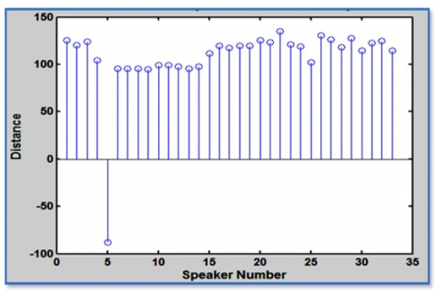
After the implementation and development of the proposed speaker recognition system, it is tested by samples of five speakers. For testing, the distance between the MFCC features of speaker number 5 and each of the other 33 speakers is calculated using BIC and shown in Figure 8. It shows that when speaker 5 is compared with itself, its value is negative; otherwise, its value is positive. A similar test is applied to our proposed method using DWT-based VSF and distance-metric BIC, and its output is shown in Figure 9.
It also shows that the value of the distance between two same speakers is negative and for different speakers is positive. The performance of the proposed system shows that the dissimilarity measure is improved as compared to the existing system.
The proposed algorithm's performance for the speaker identification system is weighed by the traditional ROC curve. In this graph, the true positive rate (missed speech rate) is plotted as a function of the false positive rate (false alarm rate) for different cut-off points. The ROC curves for two techniques are shown in Figure 10, and the AUC for these curves is calculated using Eq. (16) and given in Table 1. It is found that the proposed method covers a maximum area of 94.38% as compared to MFCC.
Figure 8. Outputs measuring the distance between speaker number 5 and all the 33 speakers using Delta BIC with MFCC
Figure 9. Outputs measuring the distance between speaker number 5 and all the 33 speakers using Delta BIC with the proposed algorithm
Figure 10. ROC curves for MFCC and proposed method using VSF
The performances of two techniques used in the ASR system have also been represented by DET curves as shown in Figure 11.
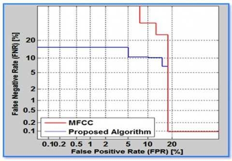
Figure 11. DET curves for MFCC and proposed algorithm based on DWT-based VSF
It is a graph of two error rates: false alarm rate and miss rate, drawn on the x and y axes, respectively. The false alarm rate is computed using Eq. (14), and the miss rate is obtained by Eq. (15). The curve for the proposed algorithm, DWT-based VSF, signified in blue, is close to the origin compared to the MFCC curve represented in red. It shows that the proposed method has lower errors than MFCC, so its performance is more accurate. The EER on the DET curve is a point where FPR and FNR are equal. The lower the EER, the better is the accuracy of the system. On the proposed method curve, the EER is obtained at 10.3564, which is less than the EER acquired using MFCC, which is 17.9487. Table 2 compares the results attained by MFCC and the proposed algorithm using ROC, DET, AUC, and EER.
Table 2. Comparison of results using ROC and DET
|
Algorithm |
Area under Curve (%) |
EER |
|
MFCC |
90.70 |
17.9487 |
|
Proposed method (wavelet based VSF) |
94.38 |
10.3564 |
5.3 Findings and their significance
The main objective of this research is to propose an efficient speaker recognition model that uses a new feature extraction technique based on DWT and VSF. This technique is named "OVSF," which successfully enhances the weak speech signal and suppresses its noise. It also effectively measures the variability of the spectrum (slowly to quickly) of the speech signal over time for different speakers. Implementation of this technique has given better results in speaker identification and verification than the existing algorithms. The scope of this novel feature algorithm is in telebanking, telephone shopping, and database access-related services where speaker’s voice features were verified and identified and then enabled to control access to the services.
This research presents an efficient feature extraction algorithm for the speaker recognition system performed on recordings of the independent speech of 33 speakers. The proposed algorithm, based on wavelet transform and VSF, is applied to extract the features of different speakers' speech signals. Initially, the Daubechies 40 (db 40) wavelet is used to compress and denoise the speech signal. Its approximation coefficient carries 99.9% of the speech information on which VSF is applied to extract its unique features that carry a multi-resolution spectrum. Next, a feature-matching technique using a traditional BIC classifier is applied for the classification of speakers. The results obtained are then represented by ROC and DET curves. The evaluation process results in four possible outcomes: TP, TN, FP, and FP. The ROC curve is drawn between the FP rate and the TP rate, while the DET curve is drawn between the FP rate and the FN rate. From these two characteristic curves, the AUC and EER are computed as 94.38 and 10.3564, respectively, for the proposed method.
The same steps of the speaker recognition process have been applied to the existing feature extraction technique, MFCC, which results in a 90.70 AUC and 17.9487 EER. Finally, the results obtained were compared, and it was found that AUC is increased and EER is reduced by using the proposed method, which is more accurate than MFCC. Segmentation and classification of small utterances of length less than five seconds in an audio recording are more challenging in the speaker diarization system. So, further research can be done on audio diarization using a new method based on OVSF.
[1] Chang, L.C., Hung, J.W. (2022). A preliminary study of robust speech feature extraction based on maximizing the probability of states in deep acoustic models. Applied System Innovation, 5(4): 71. https://doi.org/10.3390/asi5040071
[2] Chaudhary, G., Srivastava, S., Bhardwaj, S. (2017). Feature extraction methods for speaker recognition: A review. International Journal of Pattern Recognition and Artificial Intelligence, 31(12): 1750041. https://doi.org/10.1142/S0218001417500410
[3] Kabir, M.M., Mridha, M.F., Shin, J., Jahan, I., Ohi, A.Q. (2021). A survey of speaker recognition: Fundamental theories, recognition methods and opportunities. IEEE Access, 9: 79236-79263. https://doi.org/10.1109/ACCESS.2021.3084299
[4] Anusuya, M., Katti, S. (2009). Speech recognition by machine: A review. International Journal of Computer Science and Information Security, 6(3): 181-205.
[5] Hogg, A.O., Evers, C., Naylor, P.A. (2021). Multichannel overlapping speaker segmentation using multiple hypothesis tracking of acoustic and spatial features. In ICASSP 2021-2021 IEEE International Conference on Acoustics, Speech and Signal Processing (ICASSP), Toronto, ON, Canada, pp. 26-30. https://doi.org/10.1109/ICASSP39728.2021.9414130
[6] Kinnunen, T., Li, H. (2010). An overview of text-independent speaker recognition: From features to supervectors. Speech Communication, 52(1): 12-40. https://doi.org/10.1016/j.specom.2009.08.009
[7] Lee, C., Hyun, D., Choi, E., Go, J., Lee, C. (2003). Optimizing feature extraction for speech recognition. IEEE Transactions on Speech and Audio Processing, 11(1): 80-87. https://doi.org/10.1109/TSA.2002.805644
[8] Bai, Z., Zhang, X.L. (2021). Speaker recognition based on deep learning: An overview. Neural Networks, 140: 65-99. https://doi.org/10.1016/j.neunet.2021.03.004
[9] Klautau, A. (2005). The MFCC. Technical Report, Signal Processing Lab, UFPA, Brasil, pp. 1-14.
[10] Kaur, S., Sohal, J.S. (2017). Robust speaker recognition using enhanced spectrogram. International Journal of Scientific Research in Computer Science, Engineering and Information Technology, 2(4): 637-640.
[11] Huang, R., Hansen, J.H. (2006). Advances in unsupervised audio classification and segmentation for the broadcast news and NGSW corpora. IEEE Transactions on Audio, Speech, and Language Processing, 14(3): 907-919. https://doi.org/10.1109/TSA.2005.858057
[12] Rioul, O., Vetterli, M. (1991). Wavelets and signal processing. IEEE Signal Processing Magazine, 8(4): 14-38. https://doi.org/10.1109/79.91217
[13] Astuti, Y., Hidayat, R., Bejo, A. (2020). Comparison of feature extraction for speaker identification system. In 2020 3rd International Seminar on Research of Information Technology and Intelligent Systems (ISRITI), Yogyakarta, Indonesia, pp. 642-645. https://doi.org/10.1109/ISRITI51436.2020.9315332
[14] Král, P. (2010). Discrete Wavelet Transform for automatic speaker recognition. In 2010 3rd International Congress on Image and Signal Processing, Yantai, China, pp. 3514-3518. https://doi.org/10.1109/CISP.2010.5646691
[15] Ziółko, B., Manandhar, S., Wilson, R.C., Ziółko, M. (2006). Wavelet method of speech segmentation. In 2006 14th European Signal Processing Conference, Florence, Italy, pp. 1-5.
[16] Kaur, S., Sohal, J.S. (2017). Optimized speaker diarization system using discrete wavelet transform and pyknogram. International Journal on Future Revolution in Computer Science & Communication Engineering, 3(9): 52-58.
[17] Anguera, X., Bozonnet, S., Evans, N., Fredouille, C., Friedland, G., Vinyals, O. (2012). Speaker diarization: A review of recent research. IEEE Transactions on Audio, Speech, and Language Processing, 20(2): 356-370. https://doi.org/10.1109/TASL.2011.2125954
[18] Kaur, S., Sohal, J.S. (2017). Speech activity detection and its evaluation in speaker diarization system. International Journal of Computers & Technology, 16(1): 7567-7572. https://doi.org/10.24297/ijct.v16i1.5893
[19] Kaur, S., Sohal, J.S., Sharma, N. (2017). Speaker segmentation using non-linear energy operator based variance spectral flux. Current Trends in Signal Processing, 7(3): 1-6.
[20] Almpanidis, G., Kotropoulos, C. (2007). Automatic phonemic segmentation using the Bayesian information criterion with generalised gamma priors. In 2007 15th European Signal Processing Conference, Poznan, Poland, pp. 2055-2059.
[21] Perera, L.P.G., Raj, B., Flores, J.A.N. (2013). Optimization of the DET curve in speaker verification under noisy conditions. In 2013 IEEE International Conference on Acoustics, Speech and Signal Processing, Vancouver, BC, Canada, pp. 7765-7769. https://doi.org/10.1109/ICASSP.2013.6639175
[22] Fawcett, T. (2006). An introduction to ROC analysis. Pattern Recognition Letters, 27(8): 861-874. https://doi.org/10.1016/j.patrec.2005.10.010
[23] Slaby, A. (2007). ROC analysis with Matlab. In 2007 29th International Conference on Information Technology Interfaces, Cavtat, Croatia, pp. 191-196. https://doi.org/10.1109/ITI.2007.4283768
[24] Sinclair, M., King, S. (2013). Where are the challenges in speaker diarization? In 2013 IEEE International Conference on Acoustics, Speech and Signal Processing, Vancouver, BC, Canada, pp. 7741-7745. https://doi.org/10.1109/ICASSP.2013.6639170
[25] Kaur, S., Prabha, C. (2022). Performance evaluation of speaker recognition system using area under ROC curve for extracted novel features from SDM and MDM speech signals. AIP Conference Proceedings, 2555(1): 050010. https://doi.org/10.1063/5.0108925
[26] Gonen, M. (2001). Receiver Operating Characteristic (ROC) Curves. SUGI 31, Statistics and Data Analysis, Memorial Sloan-Kettering Cancer Center, pp. 1-18.
[27] Obuchi, Y. (2003). The CMU Audio Databases. http://www.speech.cs.cmu.edu/databases/pda.
[28] Hogg, A. (2021). https://github.com/ahogg/Overlapping speaker segmentation using multiple hypothesis tracking of fundamental frequency.