Annapoorani Ganesan* | Vaishali Durgamahanthi
© 2023 IIETA. This article is published by IIETA and is licensed under the CC BY 4.0 license (http://creativecommons.org/licenses/by/4.0/).
OPEN ACCESS
Breast cancer, responsible for 15% of cancer deaths among women, generally has a favorable prognosis when diagnosed early and treated appropriately. Although several standard methods for early detection are available, they present practical limitations including low sensitivity, difficulty identifying in denser breasts, radiation exposure, and cost. This study introduces a non-invasive method for breast cancer screening utilizing Electrical Impedance Tomography (EIT). Sixteen copper electrodes were strategically located evenly around the breast perimeter, and an adjacent electrode configuration was employed for current injection. The forward problem of EIT, which involves determining the electrical conductivity distribution by measuring voltages across electrodes, was addressed using finite element analysis with COMSOL Multiphysics software. The inverse problem was subsequently solved using EIDORS in MATLAB. This study considers the Gauss Newton (GN) one-step and Total Variation (TV) algorithms, and simulated outcomes were compared to identify the superior result. GN outperformed TV in anomaly detection. The results indicated that malignant tumors exhibited higher conductivity than benign ones. The segmentation technique was executed using K-means clustering, and the results pointed out the precise location and classification of small-sized tumors. The ill-posed nature of EIT was mitigated through the careful selection of appropriate electrode placement and configuration, which enhanced the stability and reliability of the results. These findings suggest that EIT could be a promising alternative for breast cancer screening, offering advantages such as high sensitivity, capability to identify tumors in denser breasts, absence of radiation exposure, and cost-effectiveness.
breast cancer screening, Electrical Impedance Tomography, COMSOL Multiphysics, finite element analysis, reconstruction, one step Gauss Newton, total variation, K-means clustering
Breast cancer (BC) is the second most common cancer in women worldwide. In fact, in 2020, it surpassed lung cancer to become the leading cause of global cancer incidence, with an estimated 2.3 million new cases, constituting 11.7% of all cancer cases. Epidemiological studies forecast that the global prevalence of BC is expected to exceed 2 million by 2030 [1]. High-income countries boast five-year survival rates for breast cancer nearing 90%, a stark contrast to middle- and low-income countries (66% in India and 40% in South Africa) [2]. The exact cause of breast cancer remains elusive, but it is widely recognized that early detection enhances survival rates. By improving the rate of early detection, we can not only reduce mortality and improve treatment outcomes but also make a substantial impact on the overall combat against breast cancer. High-precision medical imaging modalities are imperative to discern tumors in the early stages of breast cancer. This will mitigate the need for unnecessary biopsies, refine cancer treatment strategies, and improve patient survival prospects [3]. Traditional imaging modalities for screening and detecting breast cancer include mammography, B-ultrasound imaging, and magnetic resonance imaging. However, due to factors such as radiation exposure, low resolution, and high costs, a variety of imaging modalities are now being researched for breast cancer diagnostics [4-6]. The need for cost-effective, efficient, and side-effect-free breast cancer diagnostic and screening procedures has catalyzed the development of novel techniques such as thermography, EIT, infrared imaging, and optical imaging [7]. Electrical Impedance Tomography (EIT), a unique imaging technology, facilitates non-invasive, low-cost examination of biological tissues [7]. It is a technique used to determine the conductivity, permittivity, and impedance of a target [8]. By introducing a safe current into a specific area of interest in the human body and measuring the induced voltage at the boundary, one can infer the conductivity distribution within the examined region [9]. EIT leverages the distinct bioelectrical properties of tissues for identification and differentiation [10]. A common approach to achieve this is to fit data to the Cole-Cole model to generate characteristic parameters.
Permittivity / conductivity is expressed as a function of frequency by the Cole-Cole model which is given by
$\mathrm{Z}^*=R_h+\frac{\left(R_l-R_h\right)}{\left(1+\left(\mathrm{i} \frac{\mathrm{f}}{\mathrm{f}_{\mathrm{r}}}\right)^{(1-\beta)}\right)}$ (1)
where, $Z^*$ is the complex impedance $R_l$ and $R_h$ are the limiting resistance values at low and high frequencies, respectively; f is the frequency and $f_r$ is the characteristic relaxation frequency; and $\beta$ is a dispersion constant fluctuating between 0 and 1. The impedance of a breast tissue is a complex number which is expressed in both, magnitude and phase [11].
The electrical properties and structure of tissues are considered when applying EIT in clinical scenarios [12]. A three-layered forward model was proposed, consisting of thin, low-admittance layers representing skin on the top and bottom, and a thicker, high-admittance layer representing breast tissue in the middle [13]. The amplitude of the current source remains within the safe range for human detection. The medical device standard 60601-1 is adhered to by early breast cancer EIT IC [14], brain function EIT systems [15], and brain health monitoring EIT systems [16]. In line with this standard, amplitudes in the µA range are limited at frequencies up to 1 kHz, while frequencies exceeding 100 kHz are restricted to amplitudes of 10 mA [16]. A prior study proposed a 1 kHz, 0.9 mA, in vitro and in vivo FPGA and LabVIEW-based model [17], where the resistance was calculated in both the right and left breast. If the resistance change exceeds the threshold value of 50, it is classified as a breast tumor. A 16-electrode, 45 kHz, 1 mA model was proposed and utilized for experimentation with five different breast phantom shapes (in vitro), with the combined-shape approach providing improved tumor reconstruction [18]. A safe impedance measurement of the human body was conducted [19], where a current of 0.370 ± 0.003 mA with frequencies ranging from 5 to 200 kHz was employed to solve the EIT forward problem. The results demonstrate that the proposed method achieves over 90% accuracy in tumor detection in the frequency range from 10 Hz to 100 kHz. EIT techniques are categorized into three groups: adjacent, opposite, and cross, depending on the stimulation and measurement modes. The sensitivity of adjacent excitations decreases from the periphery to the center of the target [20]. A preclinical site for a cancer simulator using breast agar phantoms was developed [21], and a novel Anomaly Tracking Circle algorithm was proposed that accurately pinpoints tumor locations. Simulations for a finite element model were performed at a frequency range of 2 to 3 GHz. The percentage divergence of normal breast tissue from 7 mm of malignant tissue for resistance and reactance was found to be 1.665% and 2.174%, respectively [22]. The performance of the voltage-controlled oscillator and voltage-controlled current source used in the hardware setup was measured up to 2 MHz in the study [23]. Various resistor and capacitor combinations were tested to determine the system's accuracy. The relative error obtained was less than 0.55% across the entire range. The resulting surface potential was fed into the computer for image reconstruction using the NI USB-6259, a 16-bit, 1.25 MS/s M Series High-speed DAQ. Optical imaging was incorporated into EIT to enhance image quality by utilizing a dual-modality reconstruction approach based on optical image-guided group sparsity [24]. In a study [25], the characteristics of 12 Mexican patients were classified into two groups: electrical conductivity (3) and medical records (9). The findings of the unsupervised method show that using only electrical conductivity (43%) outperforms all available features (38%), including medical records (33%).
In EIT, surface electrodes are utilized to measure conductivity, permittivity, and impedance from various regions of the breast. By selecting suitable electrode materials and quantities, a tomographic image of the breast can be produced. Essentially, there are two types of EIT. The first is Absolute EIT, which operates based on the principle that conductivity varies among tissues. However, image reconstruction in this method is challenging due to the fact that the current traveling in the 3D path can yield multiple solutions. The second technique is Differential EIT, which is based on the movement of fluid and gas within tissues [26-28]. With multi-frequency EIT, a tomographic view of the identified parts can be obtained. EIT involves two fundamental steps: solving a forward and an inverse problem to derive specific tissue properties. The forward problem pertains to the measurement of voltage through the application of current, while the inverse problem involves the reconstruction of the original image [29].
This study addresses the ill-posed nature of EIT through the careful selection of electrode materials and configurations in solving the forward problem, with noise reduction considered. Sixteen electrodes and an adjacent pattern for current injection were used to collect the EIT data. The inverse problem was solved using a one-step Gauss-Newton method and total variation with a Noser prior. This study strives to enhance the quality of image reconstruction by effectively implementing a priori knowledge of medical imaging procedures. The structure of this paper is as follows: Section 2 provides a brief description of the analysis of the forward and inverse problem, along with simulation and experimental studies. Section 3 discusses the image reconstruction results, comparing different reconstruction algorithms. Sections 4 and 5 present the Results and Conclusion, respectively.
2.1 Analytical approach to solve the forward problem
EIT's forward problem is to determine the voltages on a breast tissue's surface given any current density distribution on the surface and conductivity distribution inside the breast. Maxwell’s equation governs the electromagnetic field created by applying a current density to the surface of a body. At low frequencies and low field strengths, they can be simplified to the generalised Laplace's equation [30]. There are numerous techniques for solving Laplace's equation. But for complex problems and complicated geometry, which is common in biomedical applications, the Finite element method is most widely used to implement the designed model under the boundary value condition for obtaining the electric potential as an output [31, 32].
The fundamental equation of EIT which is obtained from Maxwell equation is given by
$J=\sigma E$ (2)
$E=-\nabla U$ (3)
where, $\sigma$ denotes the conductivity distribution, E denotes the Electric field and U denotes the scalar voltage distribution within the field.
Combining the above two Eqs. (2) and (3):
$J=-\sigma(\nabla U)$ (4)
Assuming there are no internal current sources then:
$\nabla . J=0$ (5)
Hence,
$\nabla \cdot \sigma(\nabla \mathrm{U})=0$ (6)
The above equation represents the Partial Differential Equation for EIT Forward Problem.
Dirichlet boundary condition is given by:
$U=\frac{\mathrm{V}_1}{\mathrm{E}_1}$ (7)
Neumann boundary condition is given by:
$\sigma \frac{\partial \mathrm{u}}{\partial \mathrm{v}}=\frac{\mathrm{J}_1}{\mathrm{E}_1}$ (8)
The boundary condition for the complete electrode model used in this paper can be represented by:
$u+z_1 \sigma \frac{\partial U}{\partial V}=V_1$ on $\mathrm{E}_1, 1=1,2, \mathrm{~L}$ (9)
$\int_{\mathrm{E}_1} \sigma \frac{\partial U}{\partial V} \cdot \partial \Omega=I_l$ where $\mathrm{I}_1=1,2, \mathrm{~L}$ (10)
$\sigma \frac{\partial \mathrm{U}}{\partial \mathrm{V}}=0$ on $\Gamma / \mathrm{U}_{\mathrm{l}=1}^{\mathrm{L}} \mathrm{E}_{\mathrm{l}} \quad \mathrm{E}_{\mathrm{l}}=1,2, \mathrm{~L}$ (11)
Now, considering current density at the boundary as j then:
$j=\lceil\sigma \nabla \mathrm{U}] n_o$ (12)
where, no represents the outward normal to the boundary ∂Ω. By knowing the conductivity of the domain and electrodes, the potential distribution can be calculated.
2.2 Analysis of forward problem using COMSOL Multiphysics
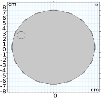
The objective of this study is to identify tumour size, tumour location, and electrode position in terms of EIT parameters. Comsol Multiphysics software and a finite element model were used to accomplish this. It employs a mathematical model by separating the boundaries into smaller, simpler components. Under frequency domain analysis, an electrical current physics interface is employed to compute the electric field and potential distribution in a 2D model of the tissue. Table 1 shows the material properties used in the modelling of a common water tank model, and Figure 1 shows the geometry of the model. Here, 16 copper electrodes were chosen and positioned evenly around the breast perimeter. NaCl was taken as a homogenous medium representing breast tissue. An anomaly was inserted as a depiction of a tumour in the tissue.
The equation for electric current interface is given by:
$\nabla . J=Q_{j . v}$ (13)
$J=\sigma E+j \omega E+J e$ (14)
The dielectric model is expressed as:
$D=\in_0 \in_r E$ (15)
The boundary current source is governed by:
$n. \left(J_1-J_2\right)=Q_{j . s}$ (16)
For frequency domain analysis:
$n. J=0$ (17)
An adjacent electrode configuration is used by supplying an alternating current of 1 mA at 50 kHz frequency to electrode 1 by using a boundary current source, and the ground is connected to the adjacent electrode (2). The voltage measurements were saved as a ".txt" file after they were recorded in the evaluation table. Now, a conducting material followed by a non-conducting material is inserted that represents a malignant and benign tumour. The experiment is repeated for both criteria, and the potential distribution is obtained.
Table 1. Material properties used in COMSOL
|
Parameters |
Conductivity σ(Sm-1) |
Geometry |
|
Homogeneous medium (Nacl) |
1.6 |
7cm |
|
Malignant tumor |
1.12 |
1cm |
|
Benign tumor |
0.5 |
1cm |
|
Electrodes (Ag) |
61.6 e6 |
Height=0.2cm Width=1cm |
The electric potential distribution in the remaining electrode pair is measured, excluding the current-carrying electrode. By using the parametric sweep option in COMSOL, the simulation is repeated by switching the current among the remaining electrodes.
Figure 1. Geometry representing the water tank model with electrodes and anomaly
A distinct difference is observed in electric field distribution and electric potential distribution for homogenous and non-homogenous media. All the readings were stored as a text file, which will be used for image reconstruction in solving the inverse problem of EIT.
2.3 Analysis of forward problem using hardware setup
Without ethical concerns, prototype development for biomedical applications cannot be directly implemented on humans. A breast-shaped plastic water tank model is taken for experimentation. Initially, silver was used as a material for electrodes; later, 16 copper electrodes were chosen for effective measurement. They are placed equidistantly on the surface of the phantom. A length of 7 cm and a width of 0.2 cm are taken as measurements of the electrode. For the study, a 0.9% w/v NaCl-saline injection is used as a homogeneous medium. A permissible current of 1 mA is applied to the first electrode, and electrode 2 is grounded. This process is repeated until all the electrodes are acting as current sources and the adjacent drive method is used for the experiment. This represents the homogeneous voltage distribution of breast tissue. A total of 256 measurements are recorded. But since the current-carrying electrode exhibits noise, readings from those electrodes were omitted, resulting in 208 measurements. An object made of plastic is inserted, and then a conducting metal is inserted, representing the benign and malignant tumours in the breast. The entire process is repeated, and the electric voltages are tabulated. From the readings obtained, the location of the tumour can be easily identified. This process is quite time-consuming due to the manual measurement of voltage and switching speeds of current electrodes.
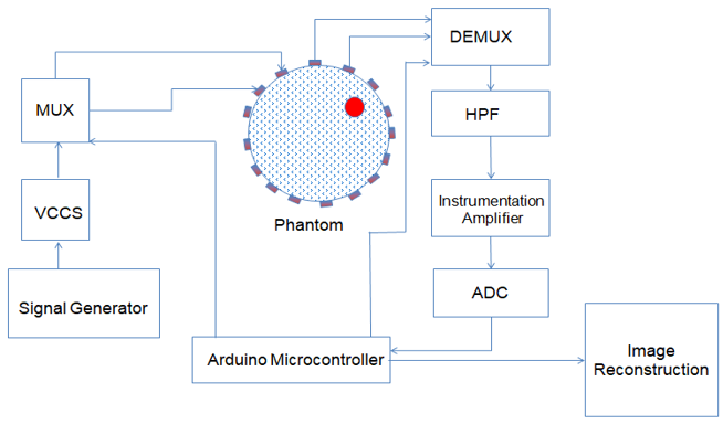
To overcome this, a design is proposed in this paper, as shown in Figure 2. Hardware components should be chosen with extreme care so that artefacts are kept to a minimum and negligible level during the design stage
Figure 2. Block diagram representation of EIT System Implementation
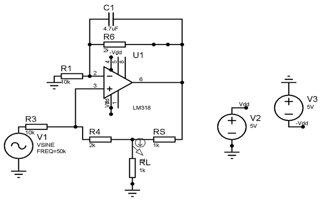
A conventional function generator can be used, or the IC2206CP can be used to generate a sine waveform. The output of this is given to the Enhanced Howland current source, which is connected using an LM318 op-amp [33]. This gives a constant current of 1 mA to the phantom, as shown in Figure 3.
Figure 3. Enhanced Howland current source
The current of 1 mA is determined by using Ohm's law.
$i_L=\frac{V_i}{p \cdot R_s}$ (18)
where,
$p=\frac{R_1}{R_2}=\frac{R_3}{R_4}$ (19)
This circuit acts as a voltage-controlled current source for the entire circuit. The switching of current between electrodes is performed by using a 16-channel analog multiplexer, CD74HC4067. Two such multiplexers are needed for inducing current and measuring voltages. The resulting measurements from breast tissue are on the order of millivolts. Any external or DC-offset noise that interferes with the signal leads to an error. Hence, these signals are sent to a high-pass filter to remove the noise caused by electrodes. Because EIT operates by difference imaging, the differences between adjacent voltages are measured by rejecting common-mode signals. The instrumentation amplifier AD620, which is shown in Figure 4, does this operation and has a high CMRR [33]. The peak detector is designed using LF 356, which is a low-noise amplifier, as shown in Figure 5. The positive half of the signal is detected and stored in a capacitor, which is given as an input to the ADC [34]. MCP3008 is used for the conversion of an analog signal to a digital signal. It has 8 channels and a sampling frequency of 200 k samples per second, which is a successive approximation type. Thus, the voltage measurements from the breast tissue are given to the controller, which is an Arduino Uno in this paper.
2.4 Analysis of the inverse problem of EIT for image reconstruction
The Image Reconstruction Algorithm plays a vital role in obtaining the final conductivity distribution of the breast tissue. Improving EIT image quality requires conservation of the region of interest, conductivity differences, and reduction of noise and artefacts [24].
Conductivity distribution and induced potential distribution are related by the following equation:
$V=F(\sigma)+\varepsilon$ (20)
where, F is a function of non-linear mapping of EIT which is given by $\mathrm{F}: \mathrm{Z}^{\mathrm{n}} \rightarrow \mathrm{Z}^{\mathrm{m}}$ and ε is the noise in measurement. The boundary voltage is represented as $\mathrm{V} \in \mathrm{Z}^{\mathrm{m}}$ and conductivity distribution as $\sigma \in \mathrm{Z}^{\mathrm{n}}$. Electrical Impedance Tomography and Diffuse Optical Reconstruction Software (EIDORS) is a MATLAB-based open-source reconstruction package. We used for solving inverse problem as it is a versatile and user-friendly platform to model, simulate, and reconstruct images of internal conductivity particularly in medical imaging and industrial processes. The inverse problem does not have a single solution but instead relies on the chosen parameters [35-37]. The one-step Gauss-Newton (GN) algorithm, when chosen as a direct linear reconstruction method, gives a satisfactory reconstruction of real-time applications. Since this is a non-iterative method, the results are computed in a short period. GN is used in conjunction with a well-known prior probability function, the NOSER prior, for an effective solution. Although the results of the GN solver give a stable solution and has faster convergence rate, the appropriate location of the tumour is not identified. Hence, we have switched to the Total Variation (TV) regularisation method, which is an iterative algorithm for solving the inverse problem of EIT. The TV regularization method is well-suited as it can provide superior reconstruction in the presence of strong inhomogeneities and noise while preserving sharp edges for accurate tumor localization.
2.5 Image segmentation
After image reconstruction, the next major operation is to find the region of interest (RoI). This is achieved by an important tool in medical image processing known as segmentation. There are five image segmentation techniques: threshold-based, region-based, edge-based, cluster-based, and watershed-based segmentation. The region-based analysis identifies regions that share a common homogeneous condition [32], whereas cluster-based analysis distinguishes clusters from the background. The K-means clustering algorithm is used in this paper as it provides promising results. It is used to segment images into clusters to locate benign and malignant tumour positions. First, it randomly selects K data points from the dataset as initial cluster centroids. Then, it assigns each data point to the nearest cluster centroid based on a chosen distance metric, such as Euclidean distance. After the assignment, the centroids of each cluster are recalculated by taking the mean of all data points assigned to that cluster. The algorithm iteratively repeats the assignment and centroid update steps until convergence or a set number of iterations.
The proposed method is evaluated by both numerical simulation and experimental set up.
3.1 Simulation results of forward problem
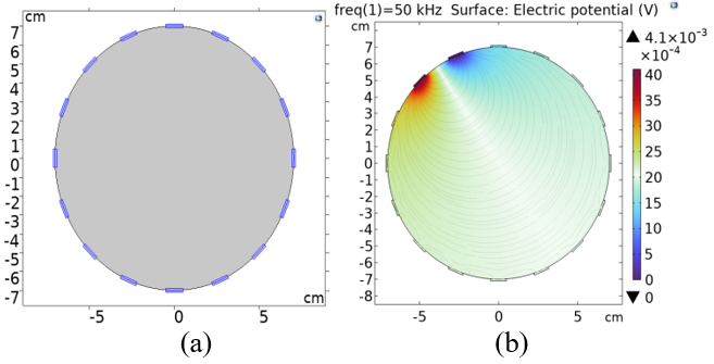
Figure 4. (a) Geometry of homogenous medium (b) Electric potential distribution of homogenous medium
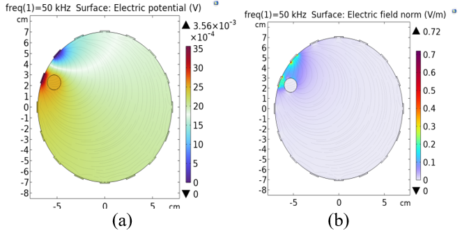
The simulation of the forward problem was carried out using COMSOL Multiphysics software. A model was created that mimics the experimental setup to check the performance of the system. The parameters of the model were chosen as mentioned in Table 1. An adjacent electrode configuration was followed, where the excitation electrode was connected to the boundary current source and the adjacent electrode was connected to the ground. The potential distribution was obtained by measuring the voltages at the remaining electrodes in the model. At a frequency of 50 kHz, a current of 1 mA was injected. The geometry was created as shown in Figure 4 (a), and the potential distribution for homogenous medium is shown in Figure 4 (b).
A 1-cm object was inserted to represent an abnormality within the medium, resulting in a heterogeneous medium. Fine meshing was done, and the conductivity of the object was chosen initially to represent a malignant tumour and then a benign tumour. Figures 5(a) and (b) represent the voltage distribution and electric field norm of a malignant tumour.
Figure 5. (a) Electric potential distribution showing malignant tumour (b) Electric field norm of malignant tumour
Figure 6. (a) Electric potential distribution showing benign tumour (b) Electric field norm of benign tumour (c) Electric potential distribution at excitation near malignant tumour (d) Electric potential distribution at excitation near benign tumour (e) Electric field norm near benign tumour
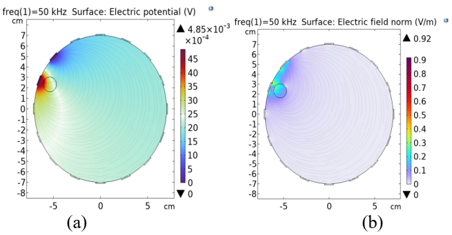
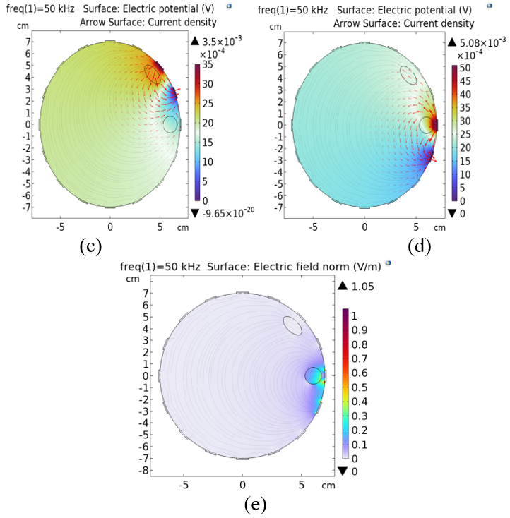
Now a non-conducting object is inserted, representing a benign tumour. The procedure is repeated, and the electric potential distribution and electric field norm of a benign tumour is represented as shown in Figures 6 (a) and (b). A condition is tested in which two anomalies are inserted, one benign and the other malignant. Figures 6 (c–e) depict the voltage and field distribution of the aforementioned model at two different excitations. The arrow plot indicated in Figures 6 (c) and (d) indicates the current absorption is higher in cancerous cells than in benign cells, where resistivity is higher.
3.2 Experimentation setup of forward problem
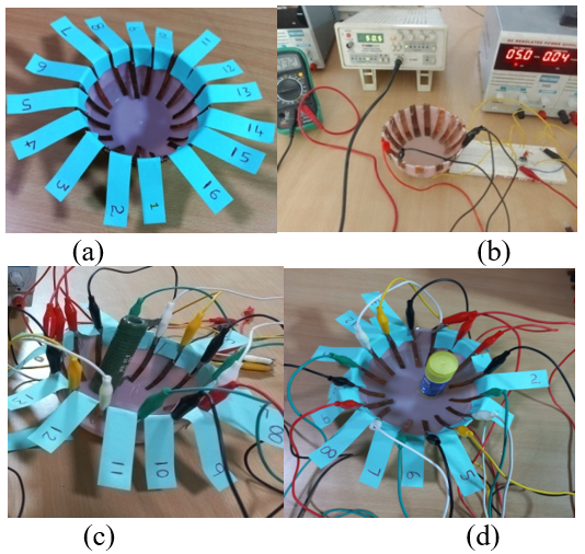
A manual experimentation setup for solving the forward problem is shown in Figure 7(a-d). Here, a plastic container in the shape of a breast is used, and NaCl solution is used as the homogenous medium. As anomalies in the medium, 1 cm of metal and 1 cm of plastic rod are inserted to make it heterogeneous. The conductivity of a metal rod is high, representing a malignant tumour, and plastic represents a benign tumour. 1 mA, 50 kHz current is injected via 16 copper electrodes through the VCCS. The experiment was carried out with both copper and silver electrodes to test the influence of electrode material. An adjacent current injection pattern is followed, where electrode 1 is connected to the positive of the VCCS and electrode 2 is connected to the ground. The experiment is repeated by switching the current injection pair (2-3, 3-4, 16-1) between electrodes until all electrodes act as excitation electrodes.
Figure 7. (a) Geometry with electrodes (b) Voltage measurements of homogenous media using copper electrodes (c) Voltage measurements of a metal object inserted as an anomaly (d) Voltage measurements of a plastic object inserted as an anomaly
3.3 Image reconstruction
The nonlinear forward operator F (σ) defined in Eq. (20) is reversed in the EIT inverse problem in order to rebuild the conductivity σ within the body Ω from a limited number of measured voltages Vm on the boundary surface. The following non-linear regularised least squares problem is a simple approach to rebuilding the conductivity data.
$f(\sigma)=\frac{h}{2} \int\left(F(\sigma)-V_m\right)^2 \partial \Omega+P(\sigma)$ (21)
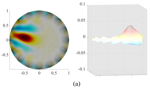
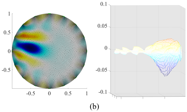
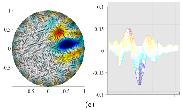
where, h is the regularisation parameter and P(σ) is the regularisation term to acknowledge the priori information about the conductivity distribution. Figure 8 (a–c) shows the image reconstructed by the one-step Gauss-Newton algorithm, where the red colour indicates higher conductivity and the blue colour indicates lower conductivity.
Figure 8. (a) Reconstructed image showing malignant tumour(left) by GN algorithm and its 3D view(right) (b) Reconstructed image showing benign tumour(left) 3D view(right) (c) Reconstructed image showing one malignant and one benign tumour by GN algorithm (left) 3D view(right)
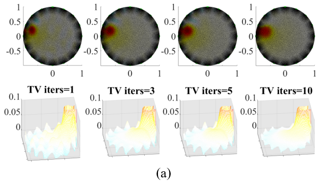
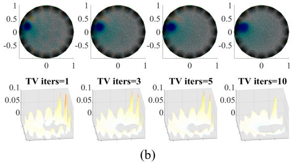
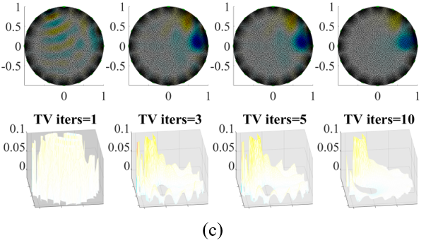
Figure 9 (a–c) shows the same image reconstructed using the total variance method for accurate reconstruction. Total variance reconstruction is an iterative process and more time-consuming than the simple Gauss-Newton algorithm. But the results give information regarding the position of the tumour.
Compared to traditional linear reconstruction methods, both the one-step Gauss-Newton and TV methods can handle nonlinear inverse problems, making them more suitable for breast cancer detection with complex tissue characteristics. The choice of the one-step Gauss-Newton and TV methods have been driven by their balance of computational efficiency, robustness to noise, and their ability to handle nonlinear inverse problems.
Figure 9. (a) Reconstructed image showing malignant tumour(top) by TV algorithm for different iterations and its 3D view(bottom) (b) Reconstructed image showing benign tumour(top) for different iterationsand its 3D view(bottom) (c) Reconstructed image showing one malignant and one benign tumour by TV algorithm(top) for different iterations and its 3D view(bottom)
3.4 Image segmentation by K-means clustering algorithm
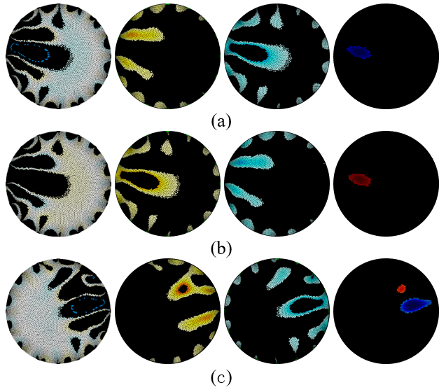
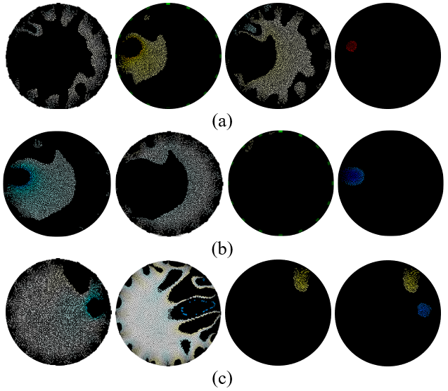
K-means clustering is an unsupervised machine learning algorithm where there is no labelled data available. The reconstructed image is loaded in MATLAB, and the number of clusters has to be given as an input (k = 4). The data points are assigned closer to the centroid, and the variance is calculated. Based on this, a new centroid is placed in the cluster, and the process is repeated until the data points are grouped into clusters. Figure 10 shows the clustering of both malignant and benign tumours reconstructed via the one-step Gauss-Newton Approach. The total variance with the pdipm algorithm with TV priori gives the exact location of tumours, which are shown in Figure 11.
Figure 10. Segmentation showing four clusters using the K-means clustering algorithm on the reconstructed image (obtained via the GN_one_step method) (a) Benign tumour (b) Malignant tumour (c) Both benign and malignant tumour
Figure 11. Segmentation using the K-means clustering algorithm showing four clusters on the reconstructed image (obtained via the TV_pdipm method) (a) Benign tumour (b) Malignant tumour (c) Both benign and malignant tumour
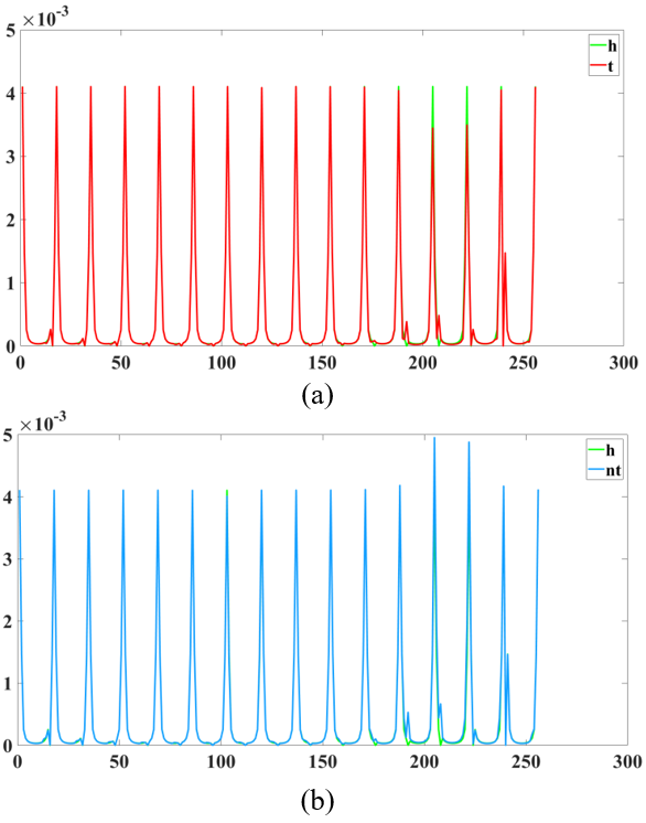
An important consideration of EIT research is modelling mistakes, which are typically brought on by a discrepancy between the forward model and the physical prototype. Errors are frequently caused by mismatched shapes and ambiguous electrode positions. In EIT-based medical imaging, where electrode placements and boundary shapes may not be fully understood and may vary over time, modelling mistakes are crucial. To address the EIT inverse problem, two different solvers were used, such as total variation (TV) and Gauss-Newton one-step (GN): NOSER. The GN algorithm performed better for identifying anomalies than the TV algorithm, which was useful for identifying smaller tumours. It was observed that increasing the repetition enhanced TV reconstruction performance. Finally, GN methods were selected and used in various tests to attain the objectives. The solution to the forward problem, which is the electric potential distribution between malignant tumour, benign tumour and homogeneous conditions, is plotted as shown in Figure 12. Malignant tumours have a smaller voltage difference than normal tissues. The output of the proposed methodology suggests that malignant tumour cells have a lower permittivity than normal cells, which the system can readily identify. Since the complexity of real breast tissue qualities cannot be fully captured by the forward problem-solving approach outlined, it is crucial to validate the suggested methodology using a larger and more varied clinical dataset. Total accuracy and specificity can be increased through comprehensive clinical validation and the use of hybrid imaging modalities.
Figure 12. Comparison of voltage differences between (a) Malignant and normal breast tissue model (b) Benign and normal breast tissue model
In this paper, Electrical Impedance Tomography for breast cancer imaging is suggested. It is low-cost, has a simple hardware implementation, and employs a non-ionizing method. The study presented in this paper demonstrates that the single-frequency sinusoidal AC signal of 50 Hz can identify even a small breast anomoly of 1cm by choosing the proper electrode configuration. EIT simulation results show that the method has the capability to classify the tissue based on conductivity and permittivity. The data are smoother and have fewer artifacts, which helps to enhance the quality of the reconstructed images and makes them better suited for breast cancer conductivity tomography imaging systems. With a hyperparameter value of 0.022, the system works faster and more effectively when a simple reconstruction algorithm, namely the Gauss-Newton one-step algorithm, is used. The final step of the color-based k-means clustering algorithm efficiently segments the anomaly with tumor classification, enabling early detection and increasing the survival rate of breast cancer patients.
[1] Mehrotra, R., Yadav, K. (2022). Breast cancer in India: Present scenario and the challenges ahead. World Journal of Clinical Oncology, 13(3): 209. https://doi.org/10.5306/wjco.v13.i3.209
[2] World Health Organization, The Global Breast Cancer Initiative. https://www.who.int/initiatives/global-breast-cancer-initiative, accessed on 26 March 2021.
[3] Chen, R., Wu, W., Qi, H., Wang, J., Wang, H. (2019). A stacked autoencoder neural network algorithm for breast cancer diagnosis with magnetic detection electrical impedance tomography. IEEE Access, 8: 5428-5437. https://doi.org/10.1109/ACCESS.2019.2961810
[4] Ma, G., Soleimani, M. (2020). Spectral capacitively coupled electrical resistivity tomography for breast cancer detection. IEEE Access, 8: 50900-50910. https://doi.org/10.1109/ACCESS.2020.2980112
[5] Chakraborty, D., Chattopadhyay, M., Bhar, R. (2013). Resistivity imaging of a phantom with irregular inhomogeneities with 32 silver electrodes based sensory system in two dimensional electrical impedance tomography. Procedia Technology, 10: 191-199. https://doi.org/10.1016/j.protcy.2013.12.352
[6] Iranmakani, S., Mortezazadeh, T., Sajadian, F., Ghaziani, M.F., Ghafari, A., Khezerloo, D., Musa, A.E. (2020). A review of various modalities in breast imaging: Technical aspects and clinical outcomes. Egyptian Journal of Radiology and Nuclear Medicine, 51(1): 1-22. https://doi.org/10.1186/s43055-020-00175-5
[7] BWarner, E. (2011). Breast-cancer screening. New England Journal of Medicine, 365(11): 1025-1032. https://doi.org/10.1056/NEJMcp1101540
[8] Shi, Y., Lou, Y., Wang, M., Tian, Z., Yang, B., Fu, F. (2022). A mismatch correction method for electrode offset in electrical impedance tomography. IEEE Sensors Journal, 22(7): 7248-7257. https://doi.org/10.1109/JSEN.2022.3155476
[9] Wu, J., Wang, P., Tang, Y., Liu, H., Wang, H., Zhang, W., Chen, L., Xu, Z., Yao, X. (2019). A new method to rapidly identify benign and malignant breast lumps through bioelectrical impedance spectroscopy. Medical Physics, 46(5): 2522-2525. https://doi.org/10.1002/mp.13474
[10] Bera, T.K., Nagaraju, J., Lubineau, G. (2016). Electrical impedance spectroscopy (EIS)-based evaluation of biological tissue phantoms to study multifrequency electrical impedance tomography (Mf-EIT) systems. Journal of Visualization, 19: 691-713. https://doi.org/10.1007/s12650-016-0351-0
[11] Zuluaga-Gomez, J., Zerhouni, N., Al Masry, Z., Devalland, C., Varnier, C. (2019). A survey of breast cancer screening techniques: Thermography and electrical impedance tomography. Journal of Medical Engineering & Technology, 43(5): 305-322. https://doi.org/10.1080/03091902.2019.1664672
[12] Miklavčič, D., Pavšelj, N., Hart, F.X. (2006). Electric Properties of Tissues. Wiley Encyclopedia of Biomedical Engineering.
[13] Kulkarni, R., Boverman, G., Isaacson, D., Saulnier, G.J., Kao, T.J., Newell, J.C. (2008). An analytical layered forward model for breasts in electrical impedance tomography. Physiological Measurement, 29(6): S27. https://doi.org/10.1088/0967-3334/29/6/S03
[14] Davidson, J.L., Wright, P., Ahsan, S.T., Robinson, R.L., Pomfrett, C.J.D., McCann, H. (2010). fEITER–a new EIT instrument for functional brain imaging. In Journal of Physics: Conference Series, 224(1): 012025.
[15] Hong, S., Lee, K., Ha, U., Kim, H., Lee, Y., Kim, Y., Yoo, H.J. (2014). A 4.9 mΩ-sensitivity mobile electrical impedance tomography IC for early breast-cancer detection system. IEEE Journal of Solid-State Circuits, 50(1): 245-257. https://doi.org/10.1109/JSSC.2014.2355835
[16] McDermott, B., O'Halloran, M., Avery, J., Porter, E. (2019). Bi-frequency symmetry difference EIT—Feasibility and limitations of application to stroke diagnosis. IEEE Journal of Biomedical and Health Informatics, 24(8): 2407-2419. https://doi.org/10.1109/JBHI.2019.2960862
[17] Mansouri, S., Alhadidi, T., Ben Azouz, M. (2020). Breast cancer detection using low-frequency bioimpedance device. Breast Cancer: Targets and Therapy, 12: 109-116. https://doi.org/10.2147/BCTT.S274421
[18] Hu, J., Soleimani, M. (2020). Combining multiple boundary shapes in deformable EIT a potential use in breast imaging. IEEE Sensors Letters, 4(4): 1-4. https://doi.org/10.1109/LSENS.2020.2978289
[19] Ain, K., Wibowo, R.A., Soelistiono, S., Muniroh, L., Ariwanto, B. (2020). Design and development of a low-cost arduino-based electrical bioimpedance spectrometer. Journal of Medical Signals and Sensors, 10(2): 125. https://doi.org/10.4103/jmss.JMSS_24_19
[20] Zhao, P.F., Fan, L.F., Wang, Y.Q., Li, Y., Wang, N., Cheng, Q., Wang, Z., Huang, L. (2022). Evaluation of electrical impedance tomography sensor using internal-external electrodes for small-scale cylindrical root zones. Measurement, 192: 110874. https://doi.org/10.1016/j.measurement.2022.110874
[21] Gutierrez-Lopez, M., Prado-Olivarez, J., Diaz-Carmona, J., Herrera-Ramírez, C.A., Gutierrez-Gnecchi, J.A., Medina-Sánchez, C.G. (2019). Electrical impedance-based methodology for locating carcinoma emulators on breast models. Journal of Sensors, 2019: 8587191. https://doi.org/10.1155/2019/8587191
[22] Tarek, M.N.A., Jalal, A.H., Alam, F., Ahad, M.A. (2018). Detection of the breast cancer based on the electrical impedance myography parameters using finite element method. In Smart Biomedical and Physiological Sensor Technology XV, 10662: 91-96. https://doi.org/10.1117/12.2307198
[23] Singh, G., Anand, S., Lall, B., Srivastava, A., Singh, V. (2018). Low-cost multifrequency electrical impedance-based system (mfeibs) for clinical imaging: Design and performance evaluation. Journal of Medical Engineering & Technology, 42(4): 274-289. https://doi.org/10.1080/03091902.2018.1478008
[24] Liu, Z., Yang, Y. (2021). Image reconstruction of electrical impedance tomography based on optical image-guided group sparsity. IEEE Sensors Journal, 21(19): 21893-21902. https://doi.org/10.1109/JSEN.2021.3104967
[25] Coripuna, R.L.R., Farías, D.I.H., Ortiz, B.O.M., Padierna, L.C., Fraga, T.C. (2021). Machine learning for the analysis of conductivity from mono frequency electrical impedance mammography as a breast cancer risk factor. IEEE Access, 9: 152397-152407. https://doi.org/10.1109/ACCESS.2021.3122948
[26] Revelo, F.A.E., Leyton, V.H.M., Rodas, C.F.R. (2020). Electrical impedance tomography: Hardware fundamentals and medical applications. Ingeniería Solidaria, 16(3). https://doi.org/10.16925/2357-6014.2020.03.02
[27] Zamora-Arellano, F., López-Bonilla, O.R., García-Guerrero, E.E., Olguín-Tiznado, J. E., Inzunza-González, E., López-Mancilla, D., Tlelo-Cuautle, E. (2020). Development of a portable, reliable and low-cost electrical impedance tomography system using an embedded system. Electronics, 10(1): 15. https://doi.org/10.3390/electronics10010015
[28] Boverman, G., Isaacson, D., Saulnier, G.J., Newell, J.C. (2009). Methods for compensating for variable electrode contact in EIT. IEEE Transactions on Biomedical Engineering, 56(12): 2762-2772. https://doi.org/10.1109/TBME.2009.2027129
[29] Dusek, J., Mikulka, J. (2021). Measurement-based domain parameter optimization in electrical impedance tomography imaging. Sensors, 21(7): 2507. https://doi.org/10.3390/s21072507
[30] Choi, M. H., Kao, T.J., Isaacson, D., Saulnier, G.J., Newell, J.C. (2007). A reconstruction algorithm for breast cancer imaging with electrical impedance tomography in mammography geometry. IEEE Transactions on Biomedical Engineering, 54(4): 700-710. https://doi.org/10.1109/TBME.2006.890139
[31] Jain, H., Isaacson, D., Edic, P.M., Newell, J.C. (1997). Electrical impedance tomography of complex conductivity distributions with noncircular boundary. IEEE Transactions on Biomedical Engineering, 44(11): 1051-1060. https://doi.org/10.1109/10.641332
[32] Hua, P., Woo, E.J., Webster, J.G., Tompkins, W.J. (1991). Iterative reconstruction methods using regularization and optimal current patterns in electrical impedance tomography. IEEE Transactions on Medical Imaging, 10(4): 621-628. https://doi.org/10.1109/42.108598
[33] Bolaños-Pérez, R., Rocha-Pérez, J.M., Díaz-Sánchez, A., Ramirez-Angulo, J., Tlelo-Cuautle, E. (2020). CMOS analog AGC for biomedical applications. Electronics, 9(5): 878. https://doi.org/10.3390/electronics9050878
[34] Farag, O., Mohamed, M., Abd El Ghany, M., Hofmann, K. (2018). Integrated sensors for early breast cancer diagnostics. In 2018 IEEE 21st International Symposium on Design and Diagnostics of Electronic Circuits & Systems (DDECS), Budapest, Hungary, pp. 153-157. https://doi.org/10.1109/DDECS.2018.00034
[35] Dimas, C., Sotiriadis, P.P. (2018). Electrical impedance tomography image reconstruction for adjacent and opposite strategy using FEMM and EIDORS simulation models. In 2018 7th International Conference on Modern Circuits and Systems Technologies (MOCAST), Thessaloniki, Greece, pp. 1-4. https://doi.org/10.1109/MOCAST.2018.8376604
[36] Reddy, V.N., Rao, P.S. (2018). Comparative analysis of breast cancer detection using K-means and FCM & EM segmentation techniques. Ingenierie des Systemes d'Information, 23(6): 173-187. https://doi.org/10.3166/isi.23.6.173-187
[37] Wongchadakul, P., Rattanadecho, P. (2021). Mathematical modeling of multilayered skin with embedded tumor through combining laser ablation and nanoparticles: Effects of laser beam area, wavelength, intensity, tumor absorption coefficient and its position. International Journal of Heat and Technology, 39(1): 89-100. https://doi.org/10.18280/ijht.390109