Chao He![]() | Yi Jia*
| Yi Jia*![]()
© 2023 IIETA. This article is published by IIETA and is licensed under the CC BY 4.0 license (http://creativecommons.org/licenses/by/4.0/).
OPEN ACCESS
Animation technology enables more accurate depth estimation and background blurring of animated scenes as it can enhance the sense of reality of the vision and increase its depth, thus it has become a hot spot in relevant research and production these days. However, although deep learning has made significant progresses in many research fields, its application in depth estimation and background blurring of animated scenes is still facing a few challenges. Most available technologies are for real world images, not animations, so there are certain difficulties capturing the unique styles of animations and their details. This study proposes two technical schemes specifically designed for animated scenes: a depth estimation model based on DenseNet, and a deblurring algorithm based on Very Deep Super Resolution (VDSR), in the hopes of providing solutions for the above mentioned matters, as well as forging more efficient and accurate tools for the animation industry.
animated scenes, depth estimation, background blurring, DenseNet, VDSR (Very Deep Super Resolution), deep learning
In the media environment of the 21st century, animations are an important form of visual art with a widespread appeal and can be frequently seen in various fields such as advertisements, films, and TV programs [1, 2]. With the help of the ever-developing animation technology, the produced animations are becoming increasingly sophisticated and complicated. To stand out in a market flooded with high-quality animation content, animators are making great efforts to create animated scenes that are more realistic and engaging [3-7], and how to accurately estimate the depth of animated scenes and blur the background to increase depth and enhance the sense of reality has become a major concern of animators and researchers. The conventional depth estimation methods require lots of manual works such as labeling and fine-tuning, while background blurring mostly relies on complex post-production procedures [8-10].
The emergence of deep learning in recent decade has revolutionized the study of image processing and computer vision [11, 12]. In this field, automatic depth estimation is now a research hot spot that has brought unprecedented opportunities for animation production. Effective depth estimation and background blurring processing can not only enhance the visual attractiveness of animations, more importantly, they can greatly improve production efficiency, reduce human intervention, and save a lot of production time and cost for animation production [13-16]. So it’s not hard to see that exploring automatic depth estimation and background blurring based on deep learning is of great practical significance for promoting the advancement of animation technology.
Although deep learning has made certain breakthroughs in many fields, its application in depth estimation and background blurring of animated scenes is yet to be further explored. Most currently available depth estimation methods are designed for real world images, their performance in dealing with animation images is not good enough, as they can not well capture the unique styles, colors, and details of the animation [17-21]. In the meantime, the current deblurring techniques are facing similar problems, and their effect in processing the animated scenes is not ideal as well [22, 23].
In view of these matters, this study attempts to propose two technical solutions designed specifically for animated scenes and verify their effect of application. At first, a DenseNet-based model is built to learn and optimize the special attributes of animation images and realize automatic depth estimation with high precision. Then, specifically for the features of animation images, a VDSR-based deblurring algorithm is proposed to effectively improve image clarity and enhance detail reproduction. Research findings of this study will contribute to improving the automation level of animation production and providing new insights for the application of deep learning in specific fields.
The automatic depth estimation model for animated scenes proposed in this study is an encoder-decoder structure model based on deep learning. This structure is designed to efficiently extract the feature information of input images, and gradually restore these feature information to the expected output images. The purpose of setting an encoder in the model is to extract features from the input images. The DenseNet network structure adopted in this study is known for its dense connection method. It ensures each layer get the information of all previous layers, so even low level features can be retained in the deeper layers of the model. In case of animated scenes, such characteristic is very valuable, since each detail in animation can greatly affect the result of depth estimation. Via fusing the features of each layer with the features of all of its previous layers, DenseNet makes sure that the extracted feature images have rich semantic information. Then, the decoder set in this model restores the expected output image from the features extracted by the encoder, and this process is realized by multiple up-sampling modules. Up-sampling not only increases resolution, but also performs high-dimensional mapping on feature images, which is conductive to restoring the depth information in images. With the help of multiple cascaded upsampling modules, the model can gradually increase the resolution of the output image while ensuring the accuracy of the depth information.
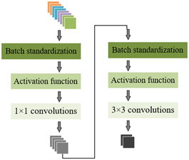
In the encoder, the core idea behind the introduction of DenseNet is to ensure that each layer can get the information of all previous layers, and this is achieved by retaining the input features in each layer and combining them with the input of current layer. Such dense connection method ensures that every node in the network receives information from the original inputs as well as from the previous layers, specifically, it consists of four DenseBlock modules and three Transition modules. DenseBlock modules are basic components of the DenseNet, which is constituted by several consecutive convolutional layers, and each layer receives the output feature images of all previous layers and takes them as the input. This design ensures maximum feature transmission and reuse. Transition modules in the DenseNet act as down-sampler and typically consist of a 1×1 convolutional layer and an average pooling layer. These modules are used between DenseBlocks to reduce the number and size of feature images. To improve computation efficiency, a Bottleneck layer has been introduced into the DenseNet. The Bottleneck layer contains 1×1 convolutions and its main objective is to reduce the number of feature images, thereby reducing the computational load of subsequent operations. Figure 1 shows the encoder structure after introducing the Bottleneck layer.
Figure 1. Encoder structure after introducing the Bottleneck layer
The decoder uses a cascade of four upsampling modules. This cascading method allows the model to gradually increase the resolution of feature images, and each step would provide contextual information for the detail restoration of depth images. At first, each upsampling module uses bi-linear interpolation to enlarge the input image by twice, then a 5×5 convolutional layer is used to decode the features. Such combination ensures that each upsampling is smooth and has abundant details.
Compared with other enlargement methods (such as nearest neighbour interpolation), the bi-linear interpolation method can enlarge images smoothly without causing obvious pixel tiles, which offers a more consecutive and consistent feature image for subsequent convolutional operations. Bi-linear interpolation is a simple calculation method that can quickly process large batches of image data. When combined with deep learning frameworks, such operation is often highly optimized, so the computation time can be reduced. In bi-linear interpolation, assuming: W11(z1,t1), W12(zm,t2), W21(z2,tm), W22(z2,t2) represent the coordinates of four neighbouring points in an animated scene image, O(z,t) represents the coordinates of the point to be solved; in this study, through bi-linear interpolation, in two different directions, linear interpolation was performed three times. At first, in one direction, linear interpolation was performed twice, and two temporary point E1(z,tm) and E2(z,t) were attained:
$d\left(E_1\right)=\frac{z_2-z}{z_2-z_1} d\left(W_{11}\right)+\frac{z-z_1}{z_2-z_1} d\left(W_{21}\right)$ (1)
$d\left(E_2\right)=\frac{z_2-z}{z_2-z_1} d\left(W_{12}\right)+\frac{z-z_1}{z_2-z_1} d\left(W_{22}\right)$ (2)
Then, in another direction, linear interpolation was performed once to get O(z,t):
$d(O)=\frac{t_2-t}{t_2-t_1} d\left(E_1\right)+\frac{t_2-t}{t_2-t_1} d\left(E_2\right)$ (3)
By combining Formulas 1 and 2, the coordinates O(z,t) of O can be attained:
$\begin{aligned} & d(z, t)=\frac{d\left(W_{11}\right)}{\left(z_2-z_1\right)\left(t_2-t_1\right)}\left(z_2-z_1\right)\left(t_2-t_1\right) +\frac{d\left(W_{21}\right)}{\left(z_2-z_1\right)\left(t_2-t_1\right)}\left(z_2-z_1\right)\left(t_2-t_1\right)+ \frac{d\left(W_{12}\right)}{\left(z_2-z_1\right)\left(t_2-t_1\right)}\left(z_2-z_1\right)\left(t_2-t_1\right)\end{aligned}$ (4)
Considering the specialties and difficulties of automatic depth estimation of animated scenes, choosing an appropriate loss function is especially important for the effectiveness of the model. Here, the model employs a combination of three types of losses: L1 loss, gradient loss, and SSIM loss. The L1 loss takes into account the absolute difference of each pixel between the predicted depth image and the real depth image. It directly measures the error between prediction and the real depth, making the model focus more on global accuracy. In terms of robustness, compared with L2 loss, L1 loss is more robust to outliers. Assuming: b represents the total number of image pixels, O represents coordinates of image pixels, then the L1 loss function is given by the following formula:
$\operatorname{LOSS}_{D E}(t, \hat{t})=\frac{1}{b} \sum_o^b\left|t_o-\hat{t}_o\right|$ (5)
The gradient loss mainly considers the pixel gradient difference between the predicted depth image and the real depth image, reflecting changes in the edge and structure of objects in the image. The contour and structure of objects are particularly important in animated scenes. The gradient loss ensures that the model has sufficient accuracy in restoring these details. Moreover, a common problem in depth estimation is that the predictions might be too smooth. Gradient loss encourages the model to produce sharper and clearer depth images. Assuming: hz represents the gradient component function of animated scene image in the horizontal direction, h* represents the gradient component function of animated scene image in the vertical direction, then the gradient loss function is given by the following formula:
$\operatorname{LOSS}_{G R}(t, \hat{t})=\sum_o^b\left|h_z\left(t_o-\hat{t}_o\right)\right|+\left|h_t\left(t_o-\hat{t}_o\right)\right|$ (6)
The SSIM index (Structural Similarity Index) measures similarities between the predicted depth image and the real depth image in terms of structure, brightness, and contrast. Unlike simple pixel-level differences, the SSIM loss focuses more on visual and structural quality of the image, and it ensures that the generated depth images are realistic for human eyes and are of high quality. In the meantime, the SSIM loss emphasizes structural consistency over a wider range of scales, which is particularly important for animated scenes, since animations usually have well-defined styles and coherent visual effect. The SSIM loss function of the network is given by the following formula:
$\operatorname{LOSS}_{S I M}(t, \hat{t})=\frac{1-\operatorname{SIM}(t, \hat{t})}{2}$ (7)
Assuming: weights of each item are hyper parameters, denoted by ηu(u=1,2,3), the total loss of the network is the weighted sum of the three kinds of losses, the function is given by the following formula:
$\begin{aligned} & \operatorname{LOSS}(t, \hat{t})=\eta_1 \operatorname{LOSS}_{D E}(t, \hat{t}) +\eta_2 \operatorname{LOSS}_{G R}(t, \hat{t})+\eta_3 \operatorname{LOSS}_{S I M}(t, \hat{t})\end{aligned}$ (8)
Figure 2. Structure of the spatial pyramid pooling module
The conventional convolutional networks generally require fixed size inputs, in contrast, Spatial Pyramid Pooling (SPP) allows the network to process input images of arbitrary size while producing output features of fixed size, and this provides a greater flexibility for images of different sizes in animated scenes. Thus, this study introduced a SPP module into the above mentioned encoder-decoder structure to ensure the features extracted from different receptive fields are integrated. In this way, richer contextual information can be captured, which is particularly important for depth estimation and image deblurring. Figure 2 gives the structure of the SPP module.
From the perspective of the traditional study of optics, blurry images of animated scenes can be caused by a range of factors including, but not limited to, motions, selection of foci, optical quality, and camera stability. These factors can be used as tools in animation production to create different visual effects and storytelling styles. For example, in photography, when an object or the camera moves during a long exposure, blurs can be created in the image due to the position changes of the object during the exposure. But in animation, motion blurs are deliberately introduced to enhance the feeling of speed and movement. They can give smoother and more natural transitions in the animation, especially in high-speed action scenes.
VDSR is a deep learning model specifically designed for super-resolution problems, and this means that its primary task is to restore high-resolution details from low-resolution images. Combined with the reasons of image blurring mentioned above, it can be seen that compared with traditional deblurring algorithms, the VDSR is better at dealing with complex blurring patterns, as it is trained on large dataset and could learn various blurring patterns and restoration skills, which enables VDSR to perform excellently in deblurring tasks, especially in cases that need to restore advanced details and textures. For instance, blurs caused by motions may result in unclear edges of objects in the image, or a part of the object might be mixed with another part of it, and VDSR can make objects in the image clearer and reduce confusion of objects as its aim is to restore high-resolution details and effectively sharpen the blurry edges.
The VDSR-based image deblurring method of animated scenes is mainly applied in the field of super-resolution. The core idea of VDSR is to use deep CNNs to capture local and global features of an image, and restore details of the high-resolution image from these features.
VDSR uses multiple convolutional layers to extract and learn image features, this allows it to capture information about an image at different levels, from lower-level features such as edges and textures to higher-level features such as the structure and scene of objects. Besides, a key characteristic of VDSR is that it adopts the residual learning method. The model mainly predicts the differences (or residuals) between low-resolution images and high-resolution images, and this enables the network to focus on recovering lost details rather than regenerating the entire image.
In animated scenes, blurring can be caused by many reasons, including blurs caused by motions and the blurring of the depth of field. By learning a large number of pairs of blurry and clear animated images, VDSR can learn to remove the blurs and restore image details. In addition, animation images differ from real world images in some aspects, such as colour saturation, and the intensity of contour lines. VDSR can adapt to these features when trained for animation images and take these factors into account during the deblurring process.
The VDSR-based deblurring method for images of animated scenes improves and adapts based on the original VDSR super-resolution structure. When it was applied to the deblurring of images of animated scenes in this study, a ResNet-based VDSR structure was introduced and the conventional CNN was adopted as the discriminative feature network.
In the ResNet structure, assuming: z represents input, D(z)represents output after activation, G(z) represents the original learning features to be learned by the network, G(z)-z represents the residuals to be learned by now, the original features to be learnt through residual learning will be changed to D(z)+z, zm+1 and zm respectively represent the input and output of the first residual unit, D represents the residual function, d represents the activation function, then the residual unit can be expressed as:
$t_U=z_U+D\left(z_U, Q_U\right)$ (9)
$z_{U+1}=d\left(t_U\right)$ (10)
Based on above formulas, the learning features corresponding to the deep level structure M can be derived further:
$z_M=z_U+\sum_{u=1}^{M-1} D\left(z_u, Q_u\right)$ (11)
Based on the chain rule of network transmission, the reverse gradient can be calculated using the following formula:
$\begin{aligned} & \frac{\partial L O S S}{\partial z_I}=\frac{\partial L O S S}{\partial z_M} \cdot \frac{\partial z_M}{\partial z_U} =\frac{\partial L O S S}{\partial z_M} \cdot\left(1+\frac{\partial}{\partial z_M} \sum_{z_M}^{M-1} D\left(z_u, Q_u\right)\right)\end{aligned}$ (12)
Since the discriminative network employs a conventional CNN structure, its goal is to distinguish between real images, un-blurred animated images, and de-blurred images generated by VDSR. Purpose of this design is to instruct the generative network to generate animated images that are close to the un-blurred real images.
Input of the generative network is the blurry images of animated scenes. The network uses multiple residual blocks for feature extraction and image restoration. Each residual block contains two convolutional layers, with a ReLU activation function followed in the middle and the short-circuit connections of input features. Figure 3 shows the structure of the generative network, and its cost function is given by the following formula:
$U_{L A R}=\frac{1}{e^2(Q G)} \sum_{z=1}^{e Q} \sum_{t=1}^{e G}\left(U_{z, t}^{G E}-H_{\varphi_H}\left(U^{M E}\right)_{z, t}\right)^2$ (13)
Figure 3. Structure of the generative network
Assuming: UAELAE represents the Mean Square Error (MSE) between the animated scene image and the image generated by the generative network, UAEGE represents value of the loss function of the generative network. To balance MSE and the network’s discrimination result about the generated image, this study used UAE to represent the entire loss function of the model, and its expression is given by the following formula:
$U^{A E}=U_{L A R}^{A E}+10^{-3} U_{G E}^{A E}$ (14)
Assuming: HϕH(UME) represents an image generated by the generative network, HϕF(HϕH(UME)) represents the probability that an image generated by the generative network is judged to be a high resolution image, the expression of UAEGE is:
$U_{G E}^{A E}=\sum_{b=1}^B-\log F_{\varphi_F}\left(H_{\varphi_H}\left(U^{M E}\right)\right)$ (15)
Figure 4. Structure of the discriminative network
Input of the discriminative network is the un-blurred real animated images or generated de-blurred images. Through the feature extraction of multiple convolutional layers, each layer is followed by a Batch Normalization and a ReLU activation function. At last, a fully connected layer is used to output the discrimination result, namely the probability that an input image is real or generated. Figure 4 gives the structure of the discriminative network. To enhance the performance of the discriminative network in identifying images of animated scenes and restoring them, parameters of the discriminative network need to be updated:
$\begin{aligned} & U_F=R_{U^{G E} \sim O_{T R}\left(U^{G E}\right)}\left[\log F_{\varphi_F}\left(U^{G E}\right)\right] +R_{U^{M E} \sim O_H\left(U^{G E}\right)}\left[\log \left(1-F_{\varphi_F}\left(H_{\varphi_H}\left(U^{G E}\right)\right)\right)\right]\end{aligned}$ (16)
Assuming: UgE represents the input image of animated scene, UAE represents the high resolution image of animated scene generated by the generative network, then, in order to reduce the loss of the deblurring model of animated scene images, HϕF(UGE) needs to be increased and HϕF(HϕH(UME)) needs to be decreased, that is, the training will update ϕF continuously.
To perform de-blurring processing on animated scene images, the method based on VDSR network is in need of an effective training strategy, and the goal of training is to ensure that the network can restore clear image details from the animation images. The training process of the VDSR network is described in detail below combining with the content and objective of this research:
1) Data preparation: first, collect a large number of animated scene images; to simulate the blurring effect, different blurring algorithms and parameters can be applied to these images to generate a group of blurry and clear image pairs, which will be taken as the training dataset. The blurry images are taken as input, and the clear images are taken as the expected output.
2) Initialization: randomly initialize the weight of the VDSR network or use the pre-trained weight.
3) Forward propagation: the blurry images of animated scenes are fed into the network and the network will try to predict its clear version.
4) Calculation of loss: use the three kinds of losses mentioned above to calculate the difference between network prediction and the real clear images, including L1 loss, gradient loss, and SSIM loss.
5) Back propagation and weight update: use the Adam optimization algorithm to update network weight based on the gradient of loss calculation, purpose of this step is to reduce the difference between the predicted image and the real image.
6) Discriminator training: for real clear images, the discriminator will judge them as “real”; while for generated images, the discriminator will judge them as “generated”. Similar to the training of the generative network, use the binary cross entropy loss to calculate the difference between the real label and the predicted label, and perform back propagation and weight update.
7) Iteration and convergence: repeat previous steps until the network converges or reaches a preset number of training rounds. Usually, the model can be considered to have converged when its performance on the validation set no longer improves or improves very slowly.
Figure 5. Loss curve of the automatic depth estimation model of animated scene images
According to the loss curve shown in Figure 5, the loss value of the DenseNet-based automatic depth estimation model of animated scene images constructed in this study can be analyze. In the figure, Experiment 1 refers to the condition of up-sampling without optimization and without introducing spatial pyramid pooling; Experiment 2 refers to the condition of up-sampling optimization; Experiment 3 refers to the condition of introducing spatial pyramid pooling; Experiment 4 refers to the condition of up-sampling optimization and with spatial pyramid pooling introduced.
As can be known from the figure, the loss values of all experiments exhibited a decreasing trend with the increase of training rounds, indicating that the model can learn and converge gradually under different settings, but the decrease speeds and the final convergence values varied from experiment to experiment. By comparing Experiment 1 and Experiment 2, it can be observed that there was a significant improvement in the loss value of the model after upsampling optimization, which emphasizes the importance of upsampling optimization in depth estimation tasks, especially when dealing with animated scene images. By comparing Experiment 1 and Experiment 3, it can be clearly seen that after introducing spatial pyramid pooling, the performance of the model has been improved further. The spatial pyramid pooling module provided the model with contextual information at different scales, so the accuracy of depth estimation has been improved. Experiment 4 was conducted under the condition with spatial pyramid pooling introduced based on upsampling optimization, judging based on the data, this combination provided the model with the best performance, so the lowest loss value was attained.
Table 1. Comparison of evaluation indicators of the automatic depth estimation model for animated scene images
|
Experiment |
Error |
Threshold Accuracy |
||||
|
Name |
MAE |
RMSE |
LMAE |
<1.25 |
<1.252 |
<1.253 |
|
Experiment 1 |
0.114 |
0.384 |
0.042 |
0.885 |
0.998 |
0.985 |
|
Experiment 2 |
0.102 |
0.379 |
0.041 |
0.879 |
0.978 |
0.983 |
|
Experiment 3 |
0.111 |
0.395 |
0.043 |
0.887 |
0.965 |
0.984 |
|
Experiment 4 |
0.097 |
0.378 |
0.038 |
0.944 |
0.971 |
0.982 |
By analyzing the data given in Table 1, it’s known that, in terms of MAE (mean absolute error), the MAE value of Experiment 4 was the lowest, only 0.097, and the MAE value of Experiment 2 was relatively low as well, indicating that the performance of Experiment 4 and Experiment 2 was relatively good in terms of prediction accuracy. As for the RMSE (root mean square error), the values of Experiment 2 and Experiment 4 were very close, both within the range of 0.37-0.38, the RMSE of Experiment 3 was the highest, which had further showed the good performance of Experiment 2 and Experiment 4 in terms of the accuracy of depth estimation. In case of LMAE (logarithmic mean absolute error), the value of Experiment 4 was the lowest, and the value of Experiment 3 was the highest, which can prove the superiority of Experiment 4 once more. In terms of the threshold of <1.25, the accuracy of Experiment 4 was the highest, reaching 0.944, which was obviously higher than other experiments. As for the thresholds of <1.252 and <1.253, the performance of Experiment 1 and Experiment 3 was better on <1.252. Overall speaking, the DenseNet-based automatic depth estimation model for animated scene images could achieve the best effect after adopting up-sampling optimization and with spatial pyramid pooling introduced, which again proved the importance of up-sampling optimization and spatial pyramid pooling to improving the depth estimation ability of the model.
Table 2 lists the entropy values of animated images processed by different methods. The entropy value of an image usually represents the information complexity of the image, the higher the entropy value, the richer the information contained in the image, and the more difficult to predict; a low entropy value indicates that the image is simpler or more uniform. On all datasets, the U-Net+CNN method gave low image entropy values, especially on the modern digital animation dataset and the animation style dataset, which means that this method might not be able to fully retain or restore the details and complexity of the original image. Compared with the U-Net+CNN method, the entropy values of the U-Net+MSN method had increased on all datasets, indicating that it can restore more image details. The GAN+MSN method gave high entropy values on all datasets, indicating that it may do a better job in restoring the details and increasing the complexity of the image. The proposed algorithm, namely the VDSR+CNN-based image deblurring algorithm for animated scenes achieved the highest image entropy value on all datasets, indicating that the proposed algorithm not only can restore details and complexity of the image, but can do better than other methods.
Table 2. Comparison of entropy after de-blurring processing of animation images
|
Method |
Entropy of Image |
|||
|
Classic animation dataset |
Modern digital animation dataset |
Animation style dataset |
Independent animation dataset |
|
|
U-Net+CNN |
6.2145 |
4.4128 |
3.2165 |
4.5538 |
|
U-Net+MSN |
7.2368 |
6.2315 |
4.7126 |
5.6742 |
|
GAN+MSN |
7.5249 |
6.6894 |
5.2684 |
6.3587 |
|
The proposed algorithm |
7.7152 |
6.8871 |
5.4158 |
7.1124 |
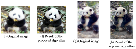
Figure 6. Comparison of de-blurring effect
Table 3. Results of NIQE quantitative comparison experiment
|
|
SRD |
NBD |
FD |
MID |
DCNND |
GFD |
BFD |
TVD |
Ours |
|
Classic animation dataset |
3.25 |
3.15 |
3.67 |
3.55 |
4.87 |
3.59 |
3.71 |
3.82 |
2.15 |
|
Modern digital animation dataset |
4.16 |
3.88 |
4.23 |
5.14 |
3.84 |
4.26 |
4.41 |
4.26 |
3.79 |
|
Animation style dataset |
3.28 |
3.26 |
4.25 |
3.26 |
3.64 |
3.58 |
3.69 |
3.74 |
3.52 |
|
Independent animation dataset |
2.75 |
2.54 |
2.68 |
4.19 |
4.18 |
2.84 |
2.81 |
3.26 |
2.48 |
After full experimental validation, the proposed method exhibited significant de-blurring effect, and Figure 6 compares the de-blurring effect. Compared with conventional de-blurring methods, the proposed method showed excellent performance in restoring details of blurry animated scenes. Judging based on the experimental results, the proposed method not only showed obvious advantages in restoring edge and texture details, but also gained satisfactory results in restoring colour and structure details.
NIQE (Natural Image Quality Evaluator) is a reference-free image quality evaluation metric used to evaluate the degree of naturalness of an image. A lower value of the degree of naturalness indicates that the quality of an image is closer to the natural state, that is, the effect of de-blurring is better. Table 3 gives the results of the NIQE quantitative comparison experiment. It can be known from the table, on the classic animation dataset, the proposed method (ours) outperformed other methods with a NIQE value of 2.15, which was much lower than that of other methods, indicating that the proposed method has an outstanding de-blurring effect on the classic animation dataset. On the modern digital animation dataset, the DCNND method attained the highest NIQE score 3.84, and the performance of the proposed method was good as well, its score was 3.79, second only to the DCNND method. On the animation style dataset, the NBD method and the MID method led the way together with a NIQE value of 3.26. Compared with other methods, the effect of the proposed method was considerable, the NIQE value was 3.52, which was equivalent to most methods. On the independent animation dataset, the de-blurring effect of the NBD method was the best, with a NIQE value of 2.54; the performance of the proposed method was not bad, its NIQE value was 2.48, indicating that on this type of datasets, the proposed method had a very good de-blurring effect.
In summary, on the four types of datasets, the proposed method achieved the best results on two datasets and its performance on the other two datasets was very close to the best results as well, which suggests that the proposed method has stable and excellent deblurring ability regardless of the type of animation dataset. When considering conventional deblurring methods (such as SRD, NBD, FD) and deep learning-based methods (such as DCNND), it can be observed that different methods have their own advantages on different datasets. This may be due to the fact that each method has their respective optimization objective and application scenario in its own design. When talking about the overall performance, the proposed method demonstrated its good applicability and excellent performance on multiple animation styles and datasets, and this has also verified the value of this study in the field of de-blurring of animation images.
This paper gave an in-depth study on automatic depth estimation and background blurring of animated scenes. Compared with the conventional images, animation images have their unique characteristics, so their processing is a challenging task. To solve the said problem, a DenseNet-based automatic depth estimation model for animated scene images was built in this paper and its performance was evaluated. Also, the generative network and discriminative network models suitable for deblurring animated images were listed, and four types of datasets (classical animation dataset, modern digital animation dataset, animation style dataset and independent animation dataset) were constructed for the de-blurring experiment of animation images.
This paper compared some evaluation indicators such as error and threshold accuracy under different experimental conditions, laying a basis for subsequent deblurring experiments. By comparing the entropy values of animation images de-blurred by different methods, the deblurring effect of each algorithm on different datasets was compared, and the de-blurring effect of various algorithms on different datasets was quantitatively compared with NIQE as the metric.
The paper not only successfully constructed a DenseNet-based automatic depth estimation model for animated scene images, but also experimentally proved that the model has a good depth estimation ability, which laid a solid foundation for deblurring experiments in the future. In the deblurring experiments, this paper considered a variety of deblurring algorithms and tested them on four different datasets. The experimental results showed that the proposed method achieved the best results on two datasets and demonstrated strong deblurring ability on other datasets as well. Especially on the classical animation dataset and the independent animation dataset, it performed particularly well. Overall speaking, this paper made a good contribution to the field of animation image deblurring. The experimental results clearly demonstrated that the proposed method is not only widely adaptable, but can attain excellent deblurring results in many scenarios.
This paper was funded by Sanjiang University "Animation major 'Scene Design' course assessment method reform and practice", (Grant No.: J22048) and Chuzhou vocational and Technical College of Humanities and social sciences "A study on the cultivation of Students' innovation literacy in Yangtze River Delta Economic Zone vocational colleges under the background of new vocational teaching methods", (Grant No.: SKZ-2022-02).
[1] Gong, J. (2022). Influence of digital media technology on animation production process. Lecture Notes in Electrical Engineering, 791: 229-236. https://doi.org/10.1007/978-981-16-4258-6_29
[2] Yu, X. (2022). Promotion and influence of motion capture technology on 3D animation production. In Conference Proceedings of the 10th International Symposium on Project Management, China, ISPM 2022, pp. 867-872.
[3] Tang, L. (2022). Application of expression capture based on image perspective analysis in animation production. In 3rd International Conference on Smart Electronics and Communication, ICOSEC 2022-Proceedings, Trichy, India, pp. 1440-1443. https://doi.org/10.1109/ICOSEC54921.2022.9951945
[4] Tian, X., Li, C. (2022). Design of multimedia teaching system for animation production based on virtual simulation experiment platform. In Proceedings-2022 14th International Conference on Measuring Technology and Mechatronics Automation, ICMTMA, Changsha, China, pp. 1187-1193. https://doi.org/10.1109/ICMTMA54903.2022.00238
[5] Zhang, Y. (2022). Computer technology-based three-dimensional animation production system management. Journal of Physics: Conference Series, 2146: 012018. https://doi.org/10.1088/1742-6596/2146/1/012018
[6] Yang, D., Liu, B., Chen, Q., Yu, S. (2022). Analysis of technological variation for animation production by remediation through genealogical approach. In 5th IEEE Eurasian Conference on Educational Innovation 2022, ECEI 2022, Taipei, Taiwan, pp. 86-89. https://doi.org/10.1109/ECEI53102.2022.9829427
[7] Zhang, Y. (2022). Application of interactive artificial intelligence in data evaluation of ink animation production. In Proceedings-International Conference on Applied Artificial Intelligence and Computing, ICAAIC 2022, Salem, India, pp. 34-37. https://doi.org/10.1109/ICAAIC53929.2022.9792862
[8] Kumar, S., Meraz, M., Chakraborty, P. (2021). Self-supervised learning of depth from sequence of images. In 2021 IEEE 8th Uttar Pradesh Section International Conference on Electrical, Electronics and Computer Engineering, UPCON 2021, Dehradun, India, pp. 1-6. https://doi.org/10.1109/UPCON52273.2021.9667660
[9] Luo, C., Yang, Z., Wang, P., Wang, Y., Xu, W., Nevatia, R., Yuille, A. (2020). Every pixel counts++: Joint learning of geometry and motion with 3d holistic understanding. IEEE Transactions on Pattern Analysis and Machine Intelligence, 42(10): 2624-2641. https://doi.org/10.1109/TPAMI.2019.2930258
[10] Mertan, A., Duff, D.J., Unal, G. (2022). Single image depth estimation: An overview. Digital Signal Processing, 123: 103441. https://doi.org/10.1016/j.dsp.2022.103441
[11] Napte, K., Mahajan, A. (2022). Deep learning based liver segmentation: A review. Revue d'Intelligence Artificielle, 36(6): 979-984. https://doi.org/10.18280/ria.360620
[12] Soufi, O., Belouadha, F.Z. (2022). Study of deep learning-based models for single image super-resolution. Revue d'Intelligence Artificielle, 36(6): 939-952. https://doi.org/10.18280/ria.360616
[13] Song, Z., Zhang, Z., Fang, F., Fan, Z., Lu, J. (2023). Deep semantic-aware remote sensing image deblurring. Signal Processing, 211: 109108. https://doi.org/10.1016/j.sigpro.2023.109108
[14] Lu, Y.C., Liu, T.P., Lin, C.H. (2023). Two-stage single image Deblurring network based on deblur kernel estimation. Multimedia Tools and Applications, 82(11): 17055-17074. https://doi.org/10.1007/s11042-022-14116-z
[15] Zhao, B., Li, W. (2023). A domain translation network with contrastive constraint for unpaired motion image deblurring. IET Image Processing, 17(10): 2866-2880. https://doi.org/10.1049/ipr2.12832
[16] Yi, S., Li, L., Liu, X., Li, J., Chen, L. (2023). HCTIRdeblur: A hybrid convolution-transformer network for single infrared image deblurring. Infrared Physics & Technology, 131: 104640. https://doi.org/10.1016/j.infrared.2023.104640
[17] Gao, W., Pu, L., Li, L., Deng, F., Bie, L. (2023). Research on depth estimation method of single aerial image. In 2023 IEEE 6th Information Technology, Networking, Electronic and Automation Control Conference (ITNEC), Chongqing, China, pp. 916-923. https://doi.org/10.1109/ITNEC56291.2023.10082076
[18] Chen, S., Fan, X., Pu, Z., Ouyang, J., Zou, B. (2022). Single image depth estimation based on sculpture strategy. Knowledge-Based Systems, 250: 109067. https://doi.org/10.1016/j.knosys.2022.109067
[19] Hidayat, M.T., Rahim, S.S., Parumo, S., A’bas, N.N., Sani, M.A.M, Aziz, H.A. (2022). Designing a two - dimensional animation for verbal apraxia therapy for children with verbal apraxia of speech. Ingénierie des Systèmes d’Information, 27(4): 645-651. https://doi.org/10.18280/isi.270415
[20] Lv, J., Qian, F., Zhang, B. (2022). Low-light image haze removal with light segmentation and nonlinear image depth estimation. IET Image Processing, 16(10): 2623-2637. https://doi.org/10.1049/ipr2.12513
[21] Tu, Y., Gao, Y., Wu, M., Qin, J. (2022). Image depth estimation algorithm based on DCGAN and prior information. In Proceedings of the 2022 5th International Conference on Telecommunications and Communication Engineering, Chengdu China, pp. 214-219. https://doi.org/10.1145/3577065.3577104
[22] Eqtedaei, A., Ahmadyfard, A. (2023). Pyramidical based image deblurring via kernel continuity prior. Circuits, Systems, and Signal Processing, 42(7): 4362-4389. https://doi.org/10.1007/s00034-023-02327-0
[23] Sharif, S.M.A., Naqvi, R.A., Ali, F., Biswas, M. (2023). DarkDeblur: Learning single-shot image deblurring in low-light condition. Expert Systems with Applications, 222: 119739. https://doi.org/10.1016/j.eswa.2023.119739