Kenan Gencol![]() | Murat Alparslan Gungor*
| Murat Alparslan Gungor*![]()
© 2023 IIETA. This article is published by IIETA and is licensed under the CC BY 4.0 license (http://creativecommons.org/licenses/by/4.0/).
OPEN ACCESS
Breast cancer, a pervasive and life-threatening malignancy, predominantly affects women worldwide. Despite the widespread adoption of imaging technologies such as mammography for early-stage breast cancer detection, access to such specialized imaging equipment remains limited in low-income countries. Conversely, ultrasound imaging has demonstrated its efficacy as a cost-effective tool for tumor identification. The advent of portable ultrasound devices facilitates rapid and precise lesion diagnosis in the breast, circumventing the need for hospital visits. Nevertheless, the images procured by portable ultrasound devices are typically necessitated to be transmitted in a compressed format for remote evaluation by physicians. This compression process often introduces artifacts in medical images, complicating the delineation of tumorous regions. To address this challenge, we introduce a deep-learning solution in this paper. A novel wavelet convolutional neural network (CNN) architecture is conceived to learn and subsequently diminish the artifacts present in compressed ultrasound images. To achieve this, a diverse dataset comprising various types of breast ultrasound images – malignant, benign, and normal – is utilized. Experimental outcomes indicate that the proposed method surpasses the denoising CNN in mitigating artifacts in compressed ultrasound images. This improved performance is particularly evident in the most compressed images, which are of significant interest. This research underscores the potential of deploying deep-learning techniques to enhance the quality of compressed medical images, thereby facilitating more accurate and efficient remote diagnoses.
breast cancer, compression, deep learning, ultrasound imaging, wavelet CNN
Breast cancer, a prevalent malignancy among women, is responsible for approximately one-sixth of all cancer-related fatalities [1, 2]. In the United Kingdom, for instance, it is the most prevalent cancer among females, with a new diagnosis occurring every ten minutes [3]. Early detection significantly increases the likelihood of successfully treating breast cancer. Various imaging technologies have been employed for the detection of this disease, with mammography being a common screening tool. However, limitations such as low sensitivity in detecting lesions in young women [4] and unnecessary costs associated with biopsies [5] have been identified. Ultrasound imaging, in comparison, offers a safer and more cost-effective alternative with higher sensitivity for detecting breast cancer lesions [6, 7]. Despite these advantages, ultrasound imaging is not devoid of drawbacks, such as the presence of speckle noise, which is currently the focus of ongoing research [8-11].
The situation in low-income countries, such as those in Africa, presents additional challenges. Women in these regions often lack access to both specialist physicians and necessary imaging devices, leading to late-stage breast cancer diagnosis [12]. This highlights the importance of portable ultrasound devices, which provide accurate and rapid diagnosis to patients unable to visit hospitals. The images obtained through these devices can either be evaluated on-site or transmitted to a distant physician for assessment.
Deep learning (DL)-based neural networks have found extensive applications in biomedical sciences, including medical image segmentation and classification [13-17]. These techniques form crucial components of medical image analysis and are indispensable for monitoring and diagnosis applications. Beyond segmentation and classification, DL techniques have also been applied successfully to medical image compression in recent years. This is especially the case for computerized tomography (CT) and magnetic resonance (MR) images, which have traditionally been compressed using transform coding methods such as JPEG and HEVC [18-22]. Despite the promising results with CT and MR images, the field of ultrasound image compression based on DL methods remains relatively unexplored. Convolutional neural networks (CNN) and generative adversarial networks (GAE) have proved their superiority in compressing CT and MR images over conventional methods [23, 24]. Several recent studies have made contributions in this area. For instance, a portable ultrasound imaging system employing a variational autoencoder (VAE) to compress pre-beamformed RF signals acquired by compressive sensing was proposed [25]. In another study, Perdios et al. [26] presented an approach for ultrasound image recovery where compression and decompression of ultrasound signals were achieved using a stacked denoising autoencoder (SDA). Moreover, China et al. introduced an ultrasound image compression system that preserves speckle information, with a CNN-based decompressor generating patho-realistic ultrasound images that convey essential information about pathological tissues [27].
As the medical images are more compressed by transform coding algorithms such as JPEG, they are exposed to higher degree of blocking artifacts. This is due to the fact that those compression algorithms operate on non-overlapping blocks of image data. Specifically, JPEG operates on 8×8 pixel blocks. Then, each block is transformed by discrete cosine transform and quantized. The quantization process creates blocking artifacts even in low compression rates. This complicates the effective identification of lesions and/or tumoral regions in medical images. The application of CNNs in the reduction of these artifacts in medical imaging is an emerging topic. To the best of our knowledge, denoising CNNs (DnCNNs) have been recently applied to the artifact reduction in electroencephalography (EEG) signals [28, 29], CT imaging [30] and digital tomosynthesis (DT) [31]. In this paper, we further advance and propose a wavelet–based CNN (WCNN) solution which reduces the blocking artifacts in compressed breast images acquired from the ultrasound device. For this purpose, we employ a publicly available dataset of malignant, benign and normal types of breast ultrasound images. Experimental results show that the proposed WCNN increases the image quality while maintaining the compression ratios, especially in the most compressed cases as desired.
The paper continues as follows: Section 2 elaborates on JPEG compression, convolutional neural networks, and the proposed wavelet CNN. Section 3 presents and discusses the experimental results. Finally, Section 4 offers concluding remarks.
In this section, we briefly introduce the JPEG compression and the CNN. Then a brief explanation of the WCNN follows. Finally, the proposed WCNN architecture is described.
2.1 JPEG compression
The JPEG image compression standard has been created by the Joint Photographic Experts Group (JPEG) and is the conventional method used in the coding of images. The specification basically consists of two parts: lossless and lossy. The lossless part just implements an entropy coding algorithm called Huffman coding. The lossy part is the mainstream of the standard (also known as the baseline mode) and implements the Discrete Cosine Transform (DCT). This transformation represents the data in a more compact form. The DCT is performed on 8×8 image blocks and the resulting DCT coefficients are scaled, truncated and quantized to reduce the dynamic range of data. The quantization step sizes of the DCT coefficients are kept in a quantization table separately. They are zigzag scanned to obtain the ordered DCT coefficients and entropy coded with the Huffman algorithm in the last stage.
The fundamental problem associated with the JPEG compression is the creation of image artifacts. As aforementioned, the baseline JPEG algorithm is lossy. Its lossy nature comes from the quantization scheme undertaken after the DCT. The DCT coefficients are further quantized to save more storage space. This quantization scheme leads to image discontinuities at the boundaries of image blocks which appear as horizontal and vertical borders between the blocks known as blocking artifacts. This phenomenon is due to the fact that this coarse quantization neglects the correlation between adjacent image blocks so that two DCT coefficients which have similar frequency characteristic in adjacent image blocks are mapped into different quantization bins. The diminishing effects of blocking artifacts are obviously visible in the final encoded image and become much more visible as the compression rate increases.
2.2 Convolutional neural network (CNN)
CNN is considered to be a deep neural network specialized in image processing tasks. These types of networks imitate the visual cortex of human brain. CNN has two subnetworks: the feature extractor network and the classifier network. The feature extractor network consists of convolution and pooling layers. Convolution layers contain convolutional filters to convert images into feature maps. Feature maps identify the unique features of the input images. In the convolutional layer, images are convolved by the filters of that layer which is followed by an activation function such as rectified linear unit (ReLU), or a leaky ReLU as given by:
$c_{i, j}^l=f\left(\sum_{m=0}^M \sum_{n=0}^N x_{i+m, j+n}^l w_{m, n}^l+b\right)$ (1)
where, xl is the input image from the previous layer, wl is the weight of the convolution filter (or kernel) of the size M×N in the current layer, b is the bias, f(.) is the activation function and cl is the output feature map calculated for all pixels at row and column (i, j)’s of the input image.
Pooling layers sub-sample the feature maps, i.e., reduce the size of the feature maps. Such kind of operation prevents a possible decrease in the network performance due to shifts, scales and distortions in the images. To achieve subsampling, max or average pooling is employed:
$p_{i, j}^l=\underset{i, j \in \Re}{\operatorname{argmax}} c_{i, j}^l \bigvee \operatorname{mean}_{i, j \in \Re} c_{i, j}^l$ (2)
where, $\mathfrak{R}$ is a region of the size 2×2, cl is the input feature map and $p_{i, j}^l$ is the output feature map. The main problem of a deepening network is the issue of overfitting. This is generally handled by the Dropout technique:
$D(x)=\left\{\begin{array}{l}\frac{x}{1-p}, \text { if } u>p \\ 0, \quad \text { otherwise }\end{array}\right\}$ (3)
where, some nodes of the network are randomly set to 0 with probability p and u represents the output of the corresponding node which is between 0 and 1. This provides some kind of regularization in the CNN and increases the generalization capability of the network. In the classifier subnetwork, a flattening fully connected layer with softmax activation function can follow the feature extractor network:
$s\left(x_i\right)=\frac{e^{x_i}}{\sum_{j=1}^K e^{x_j}}$ (4)
which maps the classifier outputs into probability values [0,1].
2.3 Wavelet CNN
When digital images are to be processed at multiple resolutions, wavelet transform (WT) is the tool of choice because WT provides powerful information regarding the spatial and frequency characteristics of the image [32]. In WT, an image is decomposed into a set of components, called subbands, which can be reassembled to reconstruct the original image without error. As shown in Figure 1, for the decomposition process, a sample image is low and high pass filtered along the columns and the outcomes of each filter are down-sampled by two. Then, each of these sub-signals is again high and low pass filtered along the rows and the outcomes obtained are once again down-sampled by two. As a result, the original image is divided into four subbands: LL (Low-Low), HH (High-High), HL (High-Low) and LH (Low-High). While the LL subband is obtained via two low pass filters and thus called the approximation subband, the HH subband is obtained via two high pass filters, called the diagonal subband. The HL and LH subbands are called vertical and horizontal subbands, respectively. Further decompositions are applied to the LL subband only in WT.
Wavelet neural networks were first introduced by Zhang et al. [33]. In this seminal study, the radial basis functions of neural networks were replaced by orthonormal wavelet scaling functions. This yielded favorably comparable performance against multilayer perceptron and radial basis function networks. For further improvement, Fujieda et al. [34] proposed wavelet convolutional neural networks (WCNNs) which combine multiresolution analysis and CNNs into one model. In this study, they formulated convolution and pooling in CNNs as filtering and downsampling to connect CNNs to multiresolution framework. They have demonstrated that WCNNs achieve better accuracy in texture classification and image annotation tasks while having fewer trainable parameters than CNNs. It is also noted that WCNNs are less prone to overfitting and require less memory. Some other variants of WCNNs were also been proposed in the following years [35-37]. Besides, Fathi et al. [38] developed a hybrid Wavelet Neural Network model, combining DWT and NARNN, for stock price forecasting. This approach ensures enhanced accuracy by first decomposing stock data with DWT. When tested on the Egyptian Exchange (EGX-30), the model outperformed other methods, showcasing its efficacy, and Oyelade et al. [39] proposed a WCNN architecture to detect the discriminative features in digital mammography for increased classification accuracy.
Figure 1. One-level decomposition of a sample image using WT
2.4 The network architecture of the proposed method
The network architecture of the proposed WCNN consists of two subnetworks: the contracting and the expanding networks. The contracting network has four wavelet decomposition layers (L, ψ) each followed by the cascade of convolution (Conv), batch normalization (BN) and activation function (ReLU) layers. The inputs to the first wavelet decomposition layer are patches of size 24×24 pixels from the images. The reason for that is JPEG is implemented by using 8×8 pixel blocks and such size of patch involves all neighboring blocks of a specific operating block to carry in sufficient image statistics for deblocking. The BN operation is used to boost the deblocking performance of the WCNN. The expanding network, reversely, has four wavelet reconstruction layers (L, ψ-1) each followed by the same Conv+BN+ReLU blocks. Differently, before the last reconstruction layer the Conv+BN+ReLU block is followed by an extra only Conv layer. In the convolution layers, 32 filters of size 3×3 with stride 2 and padding 1×1 are used to generate the desired feature maps. In the decomposition layers, we apply Haar scaling and wavelet basis functions as lowpass and highpass filters as given by:
$\phi(x, y)=\left\{\begin{array}{c}1,0 \leq x, y \leq 1 \\ 0, \text { elsewhere }\end{array}\right\}$ (5)
and
$\psi(x, y)=\left\{\begin{array}{c}1,0 \leq x, y<\frac{1}{2} \\ -1, \frac{1}{2} \leq x, y \leq 1 \\ 0, \text { elsewhere }\end{array}\right\}$ (6)
The subbands are generated by the scaling and translation of these basis functions:
$\begin{gathered}h_{j, k}(m, n)=2^{\frac{j}{2}} \phi\left(2^j m-k, 2^j n-k\right), \\ m, n \in Z, k, j \in N\end{gathered}$ (7)
$\begin{gathered}g_{j, k}(m, n)=2^{\frac{j}{2}} \psi\left(2^j m-k, 2^j n-k\right), \\ m, n \in Z, k, j \in N\end{gathered}$ (8)
where, j is the scaling factor that corresponds to downsampling and k is the translation factor which is ignored in this case. The orthonormal Haar filter coefficients in the respective subbands are:
$\begin{gathered}w_{L L}=\frac{1}{\sqrt{2}}\left[\begin{array}{ll}1 & 1 \\ 1 & 1\end{array}\right], w_{L H}=\frac{1}{\sqrt{2}}\left[\begin{array}{cc}-1 & -1 \\ 1 & 1\end{array}\right], \\ w_{H L}=\frac{1}{\sqrt{2}}\left[\begin{array}{ll}-1 & 1 \\ -1 & 1\end{array}\right], w_{H H}=\frac{1}{\sqrt{2}}\left[\begin{array}{cc}1 & -1 \\ -1 & 1\end{array}\right]\end{gathered}$ (9)
In the WCNN, filtering followed by downsampling operations of multiresolution analysis is equivalent to convolution followed by the average pooling operations. One layer of subband decomposition is accomplished using Eq. (10):
$y=(\boldsymbol{x} * \boldsymbol{w} * \boldsymbol{p}) \downarrow p$ (10)
where, x represents the input vector from the previous layer, w represents the Haar filtering kernel used as the convolution operator and p=(1/p, …, 1/p) represents the average filter with the downsampling factor p used as the average pooling operator.
The network has been trained by a random selection of size 24×24 patches for each image. It is trained for predicting the residual artifacts of the compressed images. After the residuals are predicted, it is straightforward to reconstruct the deblocked images by subtracting from the compressed images. We set 80% percent of the data as the training data and the rest as the validation data. As the optimizer algorithm, we have used Adam optimizer. Adam optimizer combines the advantages of AdaGrad and RMSProp optimization algorithms and is well-suited for problems that are in large in terms of data and parameters [40]. We set a learning rate α=0.001 with decay rates β1=0.9 and β2=0.999 and ϵ=10-8. The mini-batch size is 32 and we run 20 epochs in the training phase.
The network architecture of the proposed WCNN is illustrated in Figure 2. The hyperparameters of the proposed network are summarized in Table 1.
Table 1. Hyperparameters of the proposed WCNN
|
Parameter |
Value |
|
Input layer |
24×24 |
|
Convolution layer filter size |
3×3×1 (stride:2 padding:1) |
|
Number of filters |
32 |
|
Activation function |
ReLU |
|
Wavelet function |
Haar |
|
Mini-batch size |
32 |
|
Initial learning rate |
0.001 |
|
Number of epochs |
20 |
|
Solver algorithm |
Adam |
Figure 2. The network architecture of the proposed WCNN
We employ the publicly available dataset of breast ultrasound images obtained from female patients at the Baheya Hospital, Cairo, Egypt [41]. The images are acquired using LOGIQ E9 and LOGIQ E9 Agile ultrasound scanners. A total number of 645 breast ultrasound images, including 133 normal, 333 benign and 179 malignant type images are employed from this dataset. This dataset also provides the ground truth (image boundary) for each ultrasound image to make the ultrasound dataset beneficial. A few sample images from the dataset are depicted in Figure 3.
Compression and deblocking methods, JPEG, JPEG+CNN [42] and our method (JPEG+WCNN) are used to compress and reduce the artifacts of images. After compression and deblocking, we compare the image obtained with the reference image using the structural similarity (SSIM) index [43] to assess the performance of our method. SSIM index is used to assess the visual quality improvement of obtained images. SSIM index is a value between 0 and 1 and high values indicate better visual quality. All the experiments are carried on an Intel Core i5-based computer with 8 GB RAM and 2 GB NVIDIA GPU using MATLAB 2020B and toolboxes [44, 45].
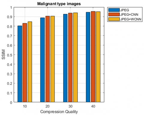
First, ultrasound images are compressed using JPEG algorithm with various compression qualities ranging from 10 (most compression case) to 40 (lowest compression case). Then, CNN and WCNN are applied to JPEG compressed images. The obtained SSIM values versus compression quality for a sample malignant type image is shown in Figure 4.
Figure 4 shows that there is a small difference between the SSIM values of the JPEG, JPEG+CNN and our method for the lowest compression case (compression quality = 40). The SSIM values of the JPEG, JPEG+CNN and our method are 0.9524, 0.9601 and 0.9655, respectively. It can be observed from Figure 4 that as the compression ratio increases, the improvement in SSIM increases and maximum improvement in SSIM happens in most compressed case (compression quality = 10). In this case, the SSIM of the JPEG, JPEG+CNN and our method are 0.8119, 0.8393 and 0.8664, respectively. The advantage of more compression is the smaller image size, while its disadvantage is more image degradation. Thus, improving the image quality after compression is very important. According to Figure 4, although the CNN improves the quality of the JPEG compressed image, our method shows the best performance among the methods.
If the important factor is the sizes of the images, we compare the sizes of the same sample malignant type image with approximately the same SSIM values obtained by the three methods as shown in Table 2. The image size reduction ratio (ISRR) in Table 2 is given as follows:
$\operatorname{ISRR}(\%)=$ $\frac{\mid \text { size of first image-size of second image } \mid}{\text { size of first image }} \times 100$ (11)
We compare the size of the images according to JPEG images thus the first image shown in Eq. (11) is the JPEG image.
As given in Table 2, while the ISRR value of JPEG+CNN is 4.8%, this value is 22.4% for the proposed method in the low compression case (SSIM value is approximately 0.96). As the compression ratio increases, the effect of the proposed method increases. For the most compressed case (SSIM value is approximately 0.86), the ISRR value of the proposed method is 37.07%, while it is 13.82% for the JPEG+CNN. Figure 5 shows the sample malignant type images with SSIM values of approximately 0.86 obtained by the JPEG, JPEG+CNN and the proposed methods. There is almost no visual difference between the images in Figure 5. The results demonstrated in Table 2 and Figure 5 prove that when the image size is important, the proposed method can be used to obtain images with the same image quality but with a smaller size. Thus, advantages such as faster image transfer, less memory requirement and faster image loading are achieved without sacrificing image quality. These advantages are especially important for ultrasound images sent to a distant physician for evaluation.
Figure 3. A montage of sample images from the dataset. From top row to bottom row: normal, benign and malignant type ultrasound images
Figure 4. The obtained SSIM values vs. compression quality for a sample malignant type image
Figure 5. Sample malignant type images with SSIM values of approximately 0.86 obtained by the methods
Up to now, we have analyzed a sample malignant type image. We perform the same analysis on 179 malignant type, 333 benign type and 133 normal type images. The average SSIM values obtained versus compression quality for these images are shown in Figure 6.
Comparing Figure 4 and Figure 6, there is no difference between the results. The proposed method shows the best performance among the methods. In particular, as the compression ratio increases, the proposed method performs better. Therefore, the proposed method allows the physician evaluating the image to make a better interpretation, as well as provides more successful image processing applications such as segmentation and classification.
While an image is compressed, it is desirable to preserve the image quality as much as possible. JPEG compression shows the worst performance in this study thus it is necessary to apply a method that improves the quality of the image after JPEG compression. Applying the well-known CNN method after JPEG compression is important to improve image quality. This study proposes a wavelet-based CNN method to improve the image quality even further. Thus, we compare the performances of JPEG, JPEG+CNN and the proposed method. The proposed method gives the best results among the methods in this study in terms of both image quality and compression performance. Especially for the high compression case, when both the quality and size of the images obtained as a result of the three methods are compared, it is observed that the performance of the proposed method is very high. Considering real-time imaging, ultrasound devices have less processing time compared to other medical imaging devices. Especially when compared to JPEG method, the proposed method has a longer processing time, which can be considered as a disadvantage for the proposed method. The future direction for this research area is to reduce the processing time without sacrificing image quality.
Table 2. Comparing the sizes of the malignant images with approximately the same SSIM values
|
Method |
JPEG |
JPEG+CNN |
Proposed Method |
|||||
|
SSIM, image size and ISRR |
SSIM |
Size |
SSIM |
Size |
ISRR (%) |
SSIM |
Size |
ISRR (%) |
|
0.8695 |
12.3 KB |
0.8648 |
10.6 KB |
13.82 |
0.8664 |
7.74 KB |
37.07 |
|
|
0.9316 |
17.8 KB |
0.9319 |
15.9 KB |
10.67 |
0.9314 |
12.6 KB |
29.21 |
|
|
0.9555 |
22.3 KB |
0.9560 |
20.6 KB |
7.62 |
0.9555 |
16.5 KB |
26.01 |
|
|
0.9654 |
25 KB |
0.9657 |
23.8 KB |
4.80 |
0.9655 |
19.4 KB |
22.4 |
|
(a)
(b)
(c)
Figure 6. The average SSIM values obtained vs. compression quality for (a) 179 malignant type images (b) 333 benign type images and (c) 133 normal type images
In this study, we have proposed a deep-learning based approach to reduce the artifacts in the JPEG-compressed breast ultrasound images. The approach is based on wavelet convolutional neural networks. The network has been trained to generate the residual artifact image. The input to the convolution layer has been selected as 24×24 pixels patches from each compressed image. Because the JPEG compression is performed on 8×8 pixels blocks, by doing that, we have covered the all neighboring blocks of an operating block and carried sufficient statistic to the convolutional layers to deblock artifacts in the input compressed image. The SSIM values of JPEG, JPEG+CNN and JPEG+WCNN images have been compared to assess the performance of the proposed approach for malignant, benign and normal ultrasound images. The results obtained show us that the proposed approach assures good performance particularly in the most compressed ones and as such we recommend it to effectively reduce artifacts in the JPEG-compressed breast ultrasound images.
[1] Ghoncheh, M., Pournamdar, Z., Salehiniya, H. (2016). Incidence and mortality and epidemiology of breast cancer in the world. Asian Pacific Journal of Cancer Prevention, 17(sup3): 43-46. https://doi.org/10.7314/APJCP.2016.17.S3.43
[2] Jemal, A., Bray, F., Center, M.M., Ferlay, J., Ward, E., Forman, D. (2011). Global cancer statistics. CA: A Cancer Journal for Clinicians, 61(2): 69-90. http://doi.org/10.3322/caac.20107
[3] Breast Cancer. https://breastcancernow.org/, accessed on March 21, 2023.
[4] Foxcroft, L.M., Evans, E.B., Porter, A.J. (2004). The diagnosis of breast cancer in women younger than 40. The Breast, 13(4): 297-306. http://doi.org/10.1016/j.breast.2004.02.012
[5] Pharoah, P.D., Sewell, B., Fitzsimmons, D., Bennett, H.S., Pashayan, N. (2013). Cost effectiveness of the NHS breast screening programme: Life table model. Bmj, 346. http://doi.org/10.1136/bmj.f2618
[6] Zhou, S., Shi, J., Zhu, J., Cai, Y., Wang, R. (2013). Shearlet-based texture feature extraction for classification of breast tumor in ultrasound image. Biomedical Signal Processing and Control, 8(6): 688-696. http://doi.org/10.1016/j.bspc.2013.06.011
[7] Jesneck, J.L., Lo, J.Y., Baker, J.A. (2007). Breast mass lesions: computer-aided diagnosis models with mammographic and sonographic descriptors. Radiology, 244(2): 390-398. http://doi.org/10.1148/radiol.2442060712
[8] Xi, X., Shi, H., Han, L., Wang, T., Ding, H.Y., Zhang, G., Tang, Y.C., Yin, Y. (2017). Breast tumor segmentation with prior knowledge learning. Neurocomputing, 237: 145-157. http://doi.org/10.1016/j.neucom.2016.09.067
[9] Huang, Q., Huang, X., Liu, L., Lin, Y., Long, X., Li, X. (2018). A case-oriented web-based training system for breast cancer diagnosis. Computer Methods and Programs in Biomedicine, 156: 73-83. http://doi.org/10.1016/j.cmpb.2017.12.028
[10] Prabusankarlal, K.M., Manavalan, R., Sivaranjani, R. (2018). An optimized non-local means filter using automated clustering based preclassification through gap statistics for speckle reduction in breast ultrasound images. Applied Computing and Informatics, 14 (1): 48-54. http://doi.org/10.1016/j.aci.2017.01.002
[11] Yap, M.H., Goyal, M., Osman, F., Martí, R., Denton, E., Juette, A., Zwiggelaar, R. (2020). Breast ultrasound region of interest detection and lesion localisation. Artificial Intelligence in Medicine, 107: 101880. http://doi.org/10.1016/j.artmed.2020.101880
[12] Foerster, M., McKenzie, F., Zietsman, A., Galukande, M., Anele, A., Adisa, C., Parham, G., Pinder, L., Schüz, J., McCormack, V., Dos-Santos-Silva, I. (2021). Dissecting the journey to breast cancer diagnosis in sub-Saharan Africa: Findings from the multicountry ABC-DO cohort study. International Journal of Cancer, 148(2): 340-351. http://doi.org/10.1002/ijc.33209
[13] Li, C., Tan, Y., Chen, W., Luo, X., He, Y., Gao, Y., Li, F. (2020). ANU-Net: Attention-based nested U-Net to exploit full resolution features for medical image segmentation. Computers & Graphics, 90: 11-20. http://doi.org/10.1016/j.cag.2020.05.003
[14] Abdolali, F., Kapur, J., Jaremko, J.L., Noga, M., Hareendranathan, A.R., Punithakumar, K. (2020). Automated thyroid nodule detection from ultrasound imaging using deep convolutional neural networks. Computers in Biology and Medicine, 122: 103871. http://doi.org/10.1016/j.compbiomed.2020.103871
[15] Rehman, A., Butt, M.A., Zaman, M. (2022). Liver Lesion Segmentation Using Deep Learning Models. Acadlore Transactions on AI and Machine Learning, 1(1): 61-67. https://doi.org/10.56578/ataiml010108
[16] Lou, A., Guan, S., Loew, M. (2023). Cfpnet-m: A light-weight encoder-decoder based network for multimodal biomedical image real-time segmentation. Computers in Biology and Medicine, 154: 106579. http://doi.org/10.1016/j.compbiomed.2023.106579
[17] Bodapati, J.D., Ahmed, S.F., Chowdary, Y.Y., Sekhar, K.R. (2023). A Deep Convolutional Neural Network Framework for Enhancing Brain Tumor Diagnosis on MRI Scans. Information Dynamics and Applications, 2(1): 42-50. https://doi.org/10.56578/ida020105
[18] Li, Z., Ramos, A., Li, Z., Osborn, M.L., Li, X., Li, Y., Yao, S.M., Xu, J. (2021). An optimized JPEG-XT-based algorithm for the lossy and lossless compression of 16-bit depth medical image. Biomedical Signal Processing and Control, 64: 102306. http://doi.org/10.1016/j.bspc.2020.102306
[19] Anitha, J., Sophia, P.E., de Albuquerque, V.H.C. (2019). Performance enhanced ripplet transform based compression method for medical images. Measurement, 144: 203-213. http://doi.org/10.1016/j.measurement.2019.04.036
[20] Parikh, S.S., Ruiz, D., Kalva, H., Fern´andez-Escribano, G., Adzic, V. (2017). High bit-depth medical image compression with hevc. IEEE Journal of Biomedical and Health Informatics, 22(2): 552-560. http://doi.org/10.1109/JBHI.2017.2660482
[21] Lucas. L.F., Rodrigues, N.M., da Silva Cruz, L.A., de Faria, S.M. (2017). Lossless compression of medical images using 3-D predictors. IEEE Transactions on Medical Imaging, 36(11): 2250-2260. http://doi.org/10.1109/TMI.2017.2714640
[22] Guarda, A.F., Santos, J.M., da Silva Cruz, L.A., Assunção, P.A., Rodrigues, N.M., de Faria, S.M. (2017). A method to improve HEVC lossless coding of volumetric medical images. Signal Processing: Image Communication, 59: 96-104. http://doi.org/10.1016/j.image.2017.02.002
[23] Mardani, M., Gong, E., Cheng, J.Y., Vasanawala, S.S., Zaharchuk, G., Xing, L., Pauly, J.M. (2018). Deep generative adversarial neural networks for compressive sensing MRI. IEEE Transactions on Medical Imaging, 38(1): 167-179. http://doi.org/10.1109/TMI.2018.2858752
[24] Guo, P., Li, D., Li, X. (2020). Deep OCT image compression with convolutional neural networks. Biomedical Optics Express, 11(7): 3543-3554. http://doi.org/10.1364/BOE.392882
[25] Gupta, S.K., Kumar, K., Seelamantula, C.S., Thakur, C.S. (2019). A portable ultrasound imaging system utilizing deep generative learning-based compressive sensing on pre-beamformed RF signals. In 2019 41st Annual International Conference of the IEEE Engineering in Medicine and Biology Society (EMBC), pp. 2740-2743. http://doi.org/10.1109/EMBC.2019.8857437
[26] Perdios, D., Besson, A., Arditi, M., Thiran, J.P. (2017). A deep learning approach to ultrasound image recovery. In 2017 IEEE International Ultrasonics Symposium (IUS), pp. 1-4. http://doi.org/10.1109/ULTSYM.2017.8092262
[27] China, D., Tom, F., Nandamuri, S., Kar, A., Srinivasan, M., Mitra, P., Sheet, D. (2019). Ultracompression: Framework for high density compression of ultrasound volumes using physics modeling deep neural networks. In 2019 IEEE 16th International Symposium on Biomedical Imaging (ISBI 2019), pp. 798-801. http://doi.org/10.1109/ISBI.2019.8759159
[28] Zhang, H., Wei, C., Zhao, M., Liu, Q., Wu, H. (2021). A novel convolutional neural network model to remove muscle artifacts from EEG. In ICASSP 2021-2021 IEEE International Conference on Acoustics, Speech and Signal Processing (ICASSP), pp. 1265-1269. http://doi.org/10.1109/ICASSP39728.2021.9414228
[29] Sun, W., Su, Y., Wu, X., Wu, X. (2020). A novel end-to-end 1D-ResCNN model to remove artifact from EEG signals. Neurocomputing, 404: 108-121. http://doi.org/10.1016/j.neucom.2020.04.029
[30] Xie, S., Zheng, X., Chen, Y., Xie, L., Liu, J., Zhang, Y., Yan, J., Zhu, H., Hu, Y. (2018). Artifact removal using improved GoogLeNet for sparse-view CT reconstruction. Scientific Reports, 8(1): 6700. http://doi.org/10.1038/s41598-018-25153-w
[31] Gomi, T., Sakai, R., Hara, H., Watanabe, Y., Mizukami, S. (2019). Development of a denoising convolutional neural network-based algorithm for metal artifact reduction in digital tomosynthesis for arthroplasty: A phantom study. PloS One, 14(9): e0222406. http://doi.org/10.1371/journal.pone.0222406
[32] Digital Image Processing Using MATLAB. Rafael C. Gonzalez, Richard E. Woods, Steven L. Eddins. Pearson Prentice Hall. 2004.
[33] Zhang, J., Walter, G.G., Miao, Y., Lee, W.N.W. (1995). Wavelet neural networks for function learning. IEEE Transactions on Signal Processing, 43(6): 1485-1497. https://doi.org/10.1109/78.388860
[34] Fujieda, S., Takayama, K., Hachisuka, T. (2018). Wavelet convolutional neural networks. arXiv preprint arXiv:1805.08620. https://arxiv.org/abs/1805.08620
[35] Liu, P., Zhang, H., Lian, W., Zuo, W. (2019). Multi-level wavelet convolutional neural networks. IEEE Access, 7: 74973-74985. http://doi.org/10.1109/ACCESS.2019.2921451
[36] Liu, J.W., Zuo, F.L., Guo, Y.X., Li, T.Y., Chen, J.M. (2021). Research on improved wavelet convolutional wavelet neural networks. Applied Intelligence, 51: 4106-4126. http://doi.org/10.1007/s10489-020-02015-5
[37] Liu, J., Li, P., Tang, X., Li, J., Chen, J. (2021). Research on improved convolutional wavelet neural network. Scientific Reports, 11(1): 17941. http://doi.org/10.1038/s41598-021-97195-6
[38] Fathi, A.Y., El-Khodary, I.A., Saafan, M. (2023). A hybrid model combining discrete wavelet transform and nonlinear autoregressive neural network for stock price prediction: An application in the Egyptian exchange. Revue d'Intelligence Artificielle, 37(1): 15-21. https://doi.org/10.18280/ria.370103
[39] Oyelade, O.N., Ezugwu, A.E. (2022). A novel wavelet decomposition and transformation convolutional neural network with data augmentation for breast cancer detection using digital mammogram. Scientific Reports, 12(1): 5913. http://doi.org/10.1038/s41598-022-09905-3
[40] Kingma, D.P., Ba, J. (2014). Adam: A method for stochastic optimization. arXiv preprint arXiv:1412.6980. https://arxiv.org/abs/1412.6980
[41] Al-Dhabyani, W., Gomaa, M., Khaled, H., Fahmy, A. (2020). Dataset of breast ultrasound images. Data in Brief, 28: 104863. http://doi.org/10.1016/j.dib.2019.104863
[42] Zhang, K., Zuo, W., Chen, Y., Meng, D., Zhang, L. (2017). Beyond a gaussian denoiser: Residual learning of deep CNN for image denoising. IEEE Transactions on Image Processing, 26(7): 3142-3155. http://doi.org/10.1109/TIP.2017.2662206
[43] Wang, Z., Bovik, A.C., Sheikh, H.R., Simoncelli, E.P. (2004). Image quality assessment: From error visibility to structural similarity. IEEE Transactions on Image Processing, 13(4): 600-612. http://doi.org/10.1109/TIP.2003.819861
[44] MatConvNet. https://www.vlfeat.org/matconvnet/, accessed on March 21, 2023.
[45] Liu, P., Zhang, H., Zhang, K., Lin, L., Zuo, W. (2018). Multi-level wavelet-CNN for image restoration. In Proceedings of the IEEE conference on computer vision and pattern recognition workshops, pp. 773-782. http://doi.org/10.1109/CVPRW.2018.00121