Rajalakshmi Somasundaram![]() | Alagumani Selvaraj
| Alagumani Selvaraj![]() | Ananthi Rajakumar
| Ananthi Rajakumar![]() | Surendran Rajendran*
| Surendran Rajendran*![]()
© 2023 IIETA. This article is published by IIETA and is licensed under the CC BY 4.0 license (http://creativecommons.org/licenses/by/4.0/).
OPEN ACCESS
The early detection of viral infections in grapevines is crucial to implement timely countermeasures and prevent the spread of disease across vineyards. This study leverages remote sensing via hyper spectral imaging to non-invasively identify and quantify infections caused by the recently discovered grapevine vein-clearing virus (GVCV), primarily during the initial asymptomatic phase. Post-calibration and preprocessing of hyper spectral images, only pixels associated with grapevines were retained. To discern between reflectance spectra profiles of healthy and GVCV-infected vines, an advanced statistical technique was employed. Subsequent to data preprocessing, an artificial hummingbird optimization technique was utilized for feature extraction, ensuring the selection of the most relevant features for enhancing the overall model classification. Furthermore, a non-invasive method was adopted to estimate the total chlorophyll (Chl) content of grape leaves. The study found a correlation between Chl concentration and the red-edge chlorophyll index, with reflectance measurements in the near-infrared (755-765 nm) and red-edge (710-720 nm) spectral ranges. For both pixel-wise and image-wise classification of disease severity, a hybrid of ZfNet+VGG19 was deployed. The proposed method, termed the Artificial Humming Bird Optimized ZfNet+VGG19 neural network (AHB_ZfNet+VGG19), demonstrated a considerable acceleration and an increase in accuracy, primarily attributed to the incorporation of prior training and model deepening. When contrasted with established methodologies, the proposed approach achieved a superior performance with an accuracy of 98.27%, precision of 97.67%, recall of 97.41% and F1-score of 97.74% for the Salinas dataset, and an accuracy of 98.45%, precision of 97.1%, recall of 97.41%, and F1-score of 97.6% for the Indian pine dataset.
chlorophyll content, grapevine viral disease, hyper spectral images, neural network optimization, artificial humming bird optimization and ZfNet+VGG19
Plant diseases have a significant negative economic impact on the worldwide agricultural industry. To avoid the spread of infection and make effective management methods possible, precision agriculture relies heavily on plant health monitoring and pathogen detection [1]. Early detection of plant pathogens and other agricultural disturbances may be a useful source of information for improving crop management strategies and disease control approaches to prevent the establishment and spreading of diseases. There are two primary categories for automated plant disease detection techniques: direct and indirect (proxy) techniques. Examples of direct detection techniques include molecular and serological techniques, which encourage high-throughput examination of several samples [2]. By identifying the disease-causing pathogens directly, these techniques accurately identify the disease-pathogen relationship [3]. Viruses, fungi, and bacteria are typical pathogens. The collection, preparation, and analysis of samples using these techniques takes at least a few days. Indirect (proxy) techniques may identify plant diseases using a range of factors, such as morphological changes, temperature change, evaporation rate reduction, and volatile compounds released by affected crops [4]. These approaches mostly depend on optical imaging technologies. The optical imaging sensors give in-depth data based on several electromagnetic spectra, allowing for the prediction of the health of the plant. Among the most popular indirect techniques for identifying plant diseases include thermography, fluorescence, and hyper spectral imaging. The characterization, detection, modelling, and categorization of plant diseases have all been accomplished with the use of hyper-spectral imaging [5]. Through the use of a hypercube, hyper-spectral imaging analyses the specular reflections from crops over the electromagnetic spectrum in thousands of small groups. The interaction of a plant with various electromagnetic spectrum regions is influenced by the biochemical elements and anatomical composition of its leaves. Due to the photosynthetic pigments in their leaves, healthy plants normally absorb light in the visible spectrum (VIS 400-700 nm). Near-infrared light scattering in the 700-1000 nm region is very sensitive to leaf cell structure [6]. Leaf water and chemical contents are the main determinants of leaf reflectance in the short-wave infrared range about SWIR 1000-2500 nm. Plants respond to diverse pressures by changing biophysically and biochemically, such as by depleting the amount of chlorophyll in the leaves or altering the cell structures of the leaves. The benefit of hyper-spectral imaging is that it can detect these minute variations in plant spectral reflectance [7]. Based on these spectral reflectance values, a variety of machine learning techniques have been created for the automated categorization of plant diseases. Typically, the process for predicting sick leaves involves extracting characteristics from spectral reflectance, building a classifier model using images of sick and normal plants, and then applying the model to new data. A common feature extraction method is the estimation of spectral Vegetation Indices (VIs) linked to specific physiological parameters. These VIs, however, often aren't made to distinguish between healthy and ill plants [8]. The amount of data in real-world scenarios makes analysis difficult. Attributes and characteristics exist in datasets. Not all features are necessary for data extraction. A model's efficiency could suffer from redundant features. Each dataset's size is decreased by feature reduction while retaining accuracy. Feature selection is a component of feature reduction. While feature selection chooses necessary features, feature extraction adds additional features from already-existing datasets. As a result, AHB is a cutting-edge meta-heuristic method that enhances accuracy. It mimics the extraordinary flight prowess and cunning feeding strategies of wild hummingbird [9]. A flexible adversarial approach is provided to enable the first strategy to generate more precise responses with greater obstacles involving two employees.
This research makes the following contributions: To achieve this, a comparative analysis is conducted between the reflectance spectra of GVCV-infected vines and normal vines, considering the datasets from each collection date. To enhance the reliability and performance of the analysis, the artificial hummingbird (AHB) feature extraction method is employed. This method strikes an improved balance between exploration and exploitation, making the newly designed algorithm more robust and efficient compared to its predecessor.
The remainder of the paper is organized as follows: The related efforts for the categorization of plant diseases using hyper spectral images are included in Section 2. The proposed neural network with classification layer is described in Section 3. The experimental analysis is presented with graphs and a comparison with two state-of-the-art techniques in Section 4. Section 5 is the conclusion and recommendations for further research conclude the essay.
Rapid viral detecting techniques based on distant and nearby optical sensors have been developed more quickly as a result of recent advancements in image and data processing technology. Thus, it is appropriate and relevant to analyse recent events. This section examines interdisciplinary approaches to hyper spectral imaging techniques, data processing, and disease classification models. According to Narayanan et al. [10], a hybrid convolution neural network (HCNN) allows the identification of banana illness, and the classification is suggested to get around these problems and help the farmers by allowing the use of fertilisers necessary for preventing the disease in its early stages. As a result, it provides better accuracy with more computational time. The held-out dataset used by Yakkundimath et al. [11], it was analysed through a threefold cross-validation procedure employing pretrained VGG-16 as well as Google Net convolutional neural network models. The average categorization accuracy for the tested VGG-16 and Google Net convolutional neural networks was 92.24% and 91.28%, accordingly.
The sensitivity of various wavelengths was explained by Cao et al. [12] using a Spectral Dilated Convolution three-dimensional Convolutional Neural Network (SDC-3DCNN) with thresholding display. The results revealed that the SDC-3DCNN model's accuracy is 95.4427% when the cumulative number of inputs is 50 characteristic wavelengths and the dilation ratio is fixed at 5. Convolutional neural networks (CNNs) and other learning frameworks, according to Nalini et al. [13], have made substantial strides in the fine-tuning of image processing to meet a database of a plant's leaves that was separately produced for various plant illnesses. It provides around 78.9% of accuracy.
A combined convolutional neural network and support vector machine (CNN-SVM) technique is suggested by Gui et al. [14] for identification of SMV. According to the experimental findings, the CNN-SVM model's training set accuracy rate was 96.67% and its training and testing accuracy rate was 94.17%. Deep convolutional neural network (DCNN) is a method suggested by Kukreja and Kumar [15] that can quickly diagnose wheat rust infections automatically without human inspection. Furthermore, our DCNN training and testing procedure yields accurate diagnosis and classification results for wheat rust illnesses. This method achieves 89.4% of accuracy with less computational time. According to Jiang et al. [16], six machine learning-assisted techniques were created based on the chosen spectral fingerprint characteristics for the early detection of anthracnose and grey mould in strawberries. According to Wang et al. [17], a novel deep learning architecture called outliers removal auxiliary classifier generative adversarial network (OR-AC-GAN) is presented. In addition to incorporating the classification function into the model, it can also uncover the inherent data characteristics and lessen the consequences of data outlier side effects.
The experiment uses the Tomato Spotted Wilt Virus (TSWV), a widespread pathogen, to validate the concept. In study of Alharbi et al. [18] employed hyperspectral remote sensing to identify grapevine viral infections early. During asymptomatic phases, it effectively recognised and categorised grapevines infected with the newly found DNA virus GVCV. Specific vegetation indicators demonstrated strong discriminating power. SVM and RF classifiers performed well in classification, while the 3D-CNN feature extractor outperformed the 2D-CNN. This method achieves 78.4% of accuracy. In study of Nguyen et al. [19] employed hyperspectral imaging to identify grapevine leafroll disease (GLD) in white and red grapevines. In greenhouse and outdoor conditions, models distinguished between sick, asymptomatic, and healthy plants with great accuracy. Here, the complexity is more.
Govender et al. [20] used Random Forest (RF) and 3D-Convolutional Neural Network (CNN) models outperformed ocular evaluation of symptoms in distinguishing infected vs. non-infected leaves. While differentiating co-infected plants was more difficult, both models demonstrated good results across all infection categories. In study [21] four machine learning algorithms were used. In 10-fold cross-validation, the boosted regression tree (BRT) model with SPA-selected wavelengths produced the best results, with 85.2% accuracy and an AUC of 0.932. The approach effectively identified TSWV at the presymptomatic stage prior to molecular identification, suggesting its potential for early detection of the virus in tobacco plants. In study [22] use of methodologies based on machine learning and modelling has shown to be beneficial in reducing the complexity of data analysis.
The training of a high number of spectral inputs and establishing their subjects is the fundamental difficulty faced by neural networks while processing hyper spectral data [23]. The use of NN classifiers for the categorization of VIs and SDIs makes this even more difficult. Overall, the Hughes effect, sometimes known as "the curse of dimensionality" is a significant challenging issue with hyper-spectral data since it involves spectral band variety and distortions. The NN modelling may be impacted by the Hughes phenomenon. It often occurs when the ratio of training pixels is higher than the required minimal to determining the quantitative fit.
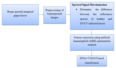
The Artificial Humming Bird Optimized ZfNet+VGG19 neural networks (AHB_ ZfNet+VGG19) used in this research are developed as seen in Figure 1. The hyper spectral photos of grapes are first captured using a wireless sensor network, then preprocessed. In order to determine the reflectance spectra of healthy and diseased leaves, the preprocessed data were subjected to a spectral signal discrimination approach. To get the best results, the artificial hummingbird (AHB) optimization approach for dimensionality reduction is used, followed by ZfNet+VGG19-based classification.
Figure 1. Block diagram of disease classification model
3.1 Network model
In this research, assume N low-altitude nodes, each with an indexing set of $X=\{1,2, \ldots X\}$. Nodes are used in the sensing of a planar area for surveillance tasks fitted with GPS, inertial measurement (IMU), webcams, detectors, and a wireless transmission interface. It is assumed that all nodes are randomly dispersed in a 3D space. With a standard constant communication range R at each place, each node may perceive a specific region. Using GPS, each node is conscious of its precise position $(a, b, c)$.
The BS, which is regarded as the target of the data packets, receives the data from UAVs that monitor the region and collect photos and video from the surveillance area. The values of $t_j=\left(a_j^{\text {uav }}, b_j^{\text {uav }}, c_j^{\text {uav }}\right)$ and $Q_i$, accordingly, provide the positional data and transmitting power of node $\mathrm{i} \in \mathrm{X}$.
To specify the network model as $G=(X, R)$, where $X$ is the node set and $R=\left\{r_1, r_2, \ldots r_n\right\}$ is the set of node locations, taking into account all node's placements and transmission strengths.
To take into account the forwarding route of $\mathrm{N}$ number of nodes for collision-free pathways. Assume that the $r_i(t)=$ $\left(a_j^{\text {uav }}(t), b_j^{\text {uav }}(t), c_j^{\text {uav }}(t)\right.$ location coordinates of node $i$ at time $t$, incorporate the forwarding route of $N$ number of nodes for collision-free pathways. Assume that the position coordinates of node $i$ at time tare $r_i(t)=\left(a_j^{\text {uav }}(t), b_j^{\text {uav }}(t), c_j^{\text {uav }}(t)\right.$, with $\forall \mathrm{i} \in\{1,2, \ldots, \mathrm{N}\}, \mathrm{t} \geq 0$.
3.2 Hyper spectral image preprocessing
The computational complexity brought on by processing the enormous volume of data is one of the difficult issues in processing high dimensional data with improved spectral and temporal resolution. In particular, this is valid for hyperspectral photographs with a wide range of spectral bands. Hyperspectral photography must be preprocessed in order to decrease the dimensions and computing complexities of the data, as well as for display and optimal band picking [24]. When compared to pixels that are far apart from one another, those with comparable spatial placements are more likely to be part of the same sort of thing. The distance between comparable pixels is nearer and more probable to convergence in the feature space. The pixels are no longer separate data points when viewed from a location within the data field. Instead, they stand for a variety of radioactive particles. Any given spot emits energy into the whole region that the picture covers. With greater distance, the energy's intensity diminishes. Every pixel collects energy from the points around it and radiates energy outward to other points. In Eq. (1), the potential energy function is determined.
$\varphi=\mathrm{m} \times \mathrm{e}^{\left(\frac{\mathrm{x}-\mathrm{y}}{\mathrm{n}}\right)^{\mathrm{k}}}$ (1)
where, $\mathrm{k}$, which in this case is set to two, indicates the Euclidean distance, $\mathrm{k} \in \mathrm{N}$ signifies the distance index, and $\mathrm{m} \geq 0$ indicates the grey value of a pixel.
he impact factor n, is a constant in the data packet that expresses the possible interaction between the pixels. Insufficient effect between the pixels results in low clustering when this factor is minimal.
In these conditions, separate pixel-centric energy zones are also described by the lines of equal potential. The interactions among individual data pixels rise as the impact factor rises, and the line features become closer together.
3.3 Spectral signal discrimination
In preprocessed hyperspectral images spatial and spectral information are available which has to be separate. Because, need only spectral signals for analysis these can be done by t-. Each independent band sample t-tests were used to analyse spectral alterations specifically attributable to that infection phase in every dataset matching to every collection date, as well as in the aggregated dataset, to determine the distinction between the reflectance spectra of normal and GVCV pathogen vines. Three t-test statistical presumptions were examined. The two groups were once thought to be independent of each other. The reflectance values of every band, which made up the dependent variable, were assumed to have a normal distribution, which was supported by evaluating the distribution's skewness (symmetry) and kurtosis (peakness). The second presumption was that the dependent variable's variance was about equal between the two groups. As a result of Levene's test returning no significant results for all bands, pooled or equal variance t-tests were employed, as shown in Eq. (2):
$\mathrm{SD}_{\mathrm{p}}^2=\frac{\left(\mathrm{n}_1-1\right) \mathrm{SD}_1^2+\left(\mathrm{n}_2-1\right) \mathrm{SD}_2^2}{\left(\mathrm{n}_1-1\right)+\left(\mathrm{n}_2-1\right)}$ (2)
The t values were determined by substituting Eq. (1) into Eq. (2):
$\frac{\mathrm{M}_1-\mathrm{M}_2}{\mathrm{SE}_{\left(\mathrm{M}_1-\mathrm{M}_2\right)}}$ where, $\mathrm{SE}_{\left(\mathrm{M}_1-\mathrm{M}_2\right)}=\sqrt{\frac{\mathrm{SD}_{\mathrm{p}}^2}{\mathrm{n}_1}}+\frac{\mathrm{SD}_{\mathrm{p}}^2}{\mathrm{n}_2}$ (3)
where, $n_1$ is the number of specimens taken from healthy vines, $M_1$ is the mean reflectance of band $i$ of normal vines, $\mathrm{M}_2$ is the meanreflectance of band $i$ of pathogens vines, and $\frac{S D_{\mathrm{p}}^2}{\mathrm{n}_2}$ is the number of specimens taken from diseased vines is $\mathrm{n}_2$, and the pooled variance is $\mathrm{SD}_{\mathrm{p}}^2$ in Eq. (3).
3.4 Artificial hummingbird optimization based feature extraction
The Artificial Hummingbird (AHB) optimization algorithm's feature extraction procedure is described. The AHB replicates the remarkable flying prowess and cunning feeding strategies of hummingbirds in the wild. Axial, diagonal, and omnidirectional foraging methods are used in this method. The goal is to simulate the hummingbird's ability to remember where food is located, directed, territorial, and migratory foraging methods are also used, along with a visiting table. The method is simple and has just a few fixed parameters that may be changed [25]. Each hummingbird in the AHB is given a distinct food source from which to feed. Hummingbirds are able to retain the location and frequency of nectar replenishment for this specific food source. It can remember the intervals between trips to each food source. The AHB has an amazing capacity to find the best solutions with these remarkable abilities. The modelling description of the AHB is demonstrated by establishing the initial population of X hummingbirds from N individuals, as seen in Eq. (4):
$X_i=L+r \times(U-L), i=1,2,3 \ldots N$ (4)
where, $L$ and $U$ denote for a D dimension's upper and lower limits, correspondingly, is a random vector with a [0, 1] range. Eq. (5) is also used to produce a visited table of food sources:
$\mathrm{VT}_{\mathrm{ij}}=\left\{\begin{array}{c}0 \text { if } \mathrm{i} \neq \mathrm{j} \\ \text { null if } \mathrm{i}=\mathrm{j}\end{array}, \mathrm{i}=1, \ldots \mathrm{N}, \mathrm{j}=1, \ldots \mathrm{N}\right.$ (5)
where, $V T_{i j}$ represents the food consumed by a hummingbird at a particular food source and becomes null if $i=j$. Moreover, they represent a hummingbird visiting a food source when $\mathrm{i} \neq \mathrm{j}$ and $\mathrm{VT}_{\mathrm{ij}}$ reach zero.
Guided Foraging-During foraging at this stage, three flying capabilities-omnidirectional, diagonal, and axial flight-are used. Eq. (6) is used to describe the axial flight
$D^{(i)}=\left\{\begin{array}{c}1, \text { if } \mathrm{i}=\operatorname{randi}([1, \mathrm{~d}]\} \mathrm{i}=1,2, \ldots \mathrm{d} \\ 0, \text { else }\end{array}\right.$ (6)
Eq. (7) may be used to represent the diagonal flight
$D^{(i)}=\left\{\begin{array}{c}1, \text { if } \mathrm{i}=\mathrm{Pp}(\mathrm{j}), \mathrm{j} \in[1, \mathrm{k}] \\ , \mathrm{Pp}=\operatorname{randperm}(\mathrm{Kp}) \\ , \mathrm{Kp} \in\left[2,\left[\mathrm{r}_1 \cdot(\mathrm{d}-2)\right]+1\right] \\ 0, \text { else } \mathrm{i}=1, \ldots . \mathrm{d}\end{array}\right.$ (7)
Eq. (8) represents the omni-directional flying.
$D^{(i)}=1 i=1,2, \ldots d$ (8)
where, rand $\mathrm{i}([1, \mathrm{~d}])$ stands for a randomly generated integer between 1 and $\mathrm{d}$, randperm $(\mathrm{k})$ for a randomly generated permutations of the values between 1 and $\mathrm{k}$, and $\mathrm{r} 1 \in[0,1]$ for a random number between 0 and 1. Eq. (9) is used to generate the directed foraging behavior
$\begin{aligned} \mathrm{V}_{\mathrm{i}}(\mathrm{t}+1)=\mathrm{X}_{\mathrm{i}, \mathrm{t}}(\mathrm{t}) & +\mathrm{a} \times \mathrm{D} \times\left(\mathrm{X}_{\mathrm{i}}(\mathrm{t})-\mathrm{X}_{\mathrm{i}, \mathrm{t}}(\mathrm{t}), \mathrm{a}\right. \in \mathrm{N}(0,1)\end{aligned}$ (9)
where, $X_{i, t}(t)$ indicates the food source $i$ for $t$ iteration. The hummingbirds' preferred food source is $\mathrm{X}_{\mathrm{i}, \mathrm{t}}(\mathrm{t})$.
Territorial Foraging-A hummingbird is highly possible to look for a new food source rather than to visit other existing food sources when flower nectar runs out. A hummingbird may therefore effortlessly fly to a nearby location inside its region where it can discover a potentially superior food source. Eq. (10) is used to represent the situation
$V_i(t+1)=X_{i, t}(t)+b \times D \times X_i(t), b \in N(0,1)$ (10)
Migration Foraging-A hummingbird will travel to a different eating area if its favorite spot runs out of food. The visit table will change when this hummingbird switches from its prior food source to the new one. The migratory of a hummingbird from a nectar source with the fewest nectar replenishments to the one with a randomized rate of nectar generation is described Eq. (11).
$\mathrm{X}_{\mathrm{W}}(\mathrm{t}+1)=\mathrm{L}+\mathrm{r} \times(\mathrm{U}-\mathrm{L})$ (11)
The food supply with the least fitness value is represented by Xw in this case. The visiting table is a key part of the AHA technique. Eq. (12) used to update the visiting table for every hummingbird.
$\begin{gathered}\mathrm{VT}_{\mathrm{i}, \mathrm{k}}=\mathrm{VT}_{\mathrm{i}, \mathrm{k}}+1, \text { if } \mathrm{k} \neq \mathrm{i} \text { and } \mathrm{k} \neq \operatorname{target}, \mathrm{k} =1,2 \ldots \mathrm{h}_{\mathrm{n}}\end{gathered}$ (12)
The time that the same hummingbirds visited each food source is shown in this visiting table. A high number of visits is indicated by a lengthy time between visits.
3.5 Chlorophyll estimation
A conceptual approach was created to quantify the concentration of plant pigments such total chlorophyll, anthocyanins, and carotenoids using three distinct spectral bands. In three spectral bands $\tau i$, the model establishes a relationship between the target pigment and leaf reflectance $\rho_{\tau \mathrm{i}}$ in Eq. (13):
$\text{pigment contnet} \propto a_{\text {pigment }}=\left(\rho_{\tau \mathrm{i}_n}^{-1}-\rho_{\tau 2 n}^{-1}\right) \times \rho_{\tau 3 n}^{-1}
$ (13)
where, $a_{\text {pigment }}$ is the relevant pigment's absorption coefficient. In the tiband of the spectrum, reflectance is most sensitive to the absorption of the color of interest; however, other pigments' absorbing and leaf scatters also have an impact.
Depending on which $\lambda 1$ was chosen, there were two different approaches to estimate $\mathrm{Chl}$ using the three-band model of Eq. (14). As a result, the following types of chlorophyll indices (CI) have been proposed.
$\mathrm{CI}_{\text {green }}=\frac{\mathrm{P}_{\text {NIR }}}{\mathrm{P}_{\text {green }}}-1$ (14)
$\mathrm{CI}_{\text {red edge }}=\frac{\mathrm{P}_{\mathrm{NIR}}}{\mathrm{P}_{\mathrm{r} 4 \mathrm{ed} \text { edge }}}-1$ (15)
It was discovered that $\mathrm{CI}_{\text {green }}$ is only a reliable indicator of chlorophyll concentration in leaves lacking of anthocyanin IN Eq. (15). Anthocyanin consumes in situ at around 550nm; as a result, if $\rho \lambda 1$ is near 550nm in the green band, the index will be significantly impacted by the absorption of both anthocyanin and Chl. The amount of $\mathrm{Chl}$ was overestimated. In order to estimate Chl in leaves that contain anthocyanins, it was recommended to utilize the $\mathrm{CI}_{\text {red edge }}$.
3.6 ZfNet+VGG19 based classification
Figure 2. Architecture of ZfNet+VGG19
This section introduces the categorization procedure utilizing a pretrained CNN. Three layers make up a CNN: a convolutional layer, a pooling layer, and a fully connected layer. Computer vision activities including picture creation, image classification, image captioning, and many more may be performed using four pretrained networks. VGG19 and ZfNet were two of these pretrained networks utilized in this research. For layer-by-layer convolutional network visualization and comprehension, ZfNet+VGG19 is utilized. The network used batch stochastic gradient descent for training and ReLUs for activation. ZfNet+VGG19 architecture considerably outperforms AlexNet by dissecting the convolutional network layer by layer, changing the layer hyper-parameters like filter size or stride, and successfully reducing the error rates. The model architecture of a deep convolutional neural network is shown in Figure 2. The depth of the network depends on the number of hidden layers. Hidden layers are those layers that exist between the input and output layers. It has 3 completely connected layers, max-pooling layers, and 5 shared convolutional layers.
The dataset was separated into a training and testing dataset for every class after just a feature extraction process. It comprises of training and testing pictures for DS1, DS2, DS3, and DS4 of 2452, 4238, 4011, and 10292 photos and 584, 1971, 1357, and 3912 images, accordingly. The complete dataset that serves as the input for the model was downsized to 224×224 pixels. Based on the number of categories, the output of the final completely linked layer was divided into 5 groups. It calculated and recorded the average value that had exponentially depreciated in the two instances before it and calculated the averaged of the prior gradients that had depreciated exponentially.
Pooling layer: This is employed to reduce the spatial domain and hence the network's calculation after the convolution layer. Typically, the kernel size in ZfNet+VGG19 is 2×2 with stride 2. In this case, the pooling layer executes the maximum operation across the restricted spatial area R, yielding a feature map in Eq. (16):
$\mathrm{p}^{\mathrm{l}}=\max _{\mathrm{i} \in \mathrm{R}} \alpha_{\mathrm{i}}^{\mathrm{l}}$ (16)
Fully connected (FC) layer: In ZfNet+VGG19, FC are emulated employing a convolution with a size of n1, n2, where n1×n2 are the sizes of the input and output tensors, accordingly. In most cases, n1 is an integer and n2 is a triplet (7×7×512).
Dropout: This layer, which is also known as "Drop," is often used to reduce the input fit and enhance the DL algorithm's hypothesis. Typically, it gives the network nodes weights (in PDCNN the percentage of 0.5 is assigned to the two drop layers).
Softmax: A ReLU layer accompanies the DL model with several layers and a convolution layer, establishing the nonlinearity in the ZfNet+VGG19 model, and is often represented as “$\sigma$”.
The categorization of the grape picture to $3-\mathrm{D}$ groups has been performed along with the borders. The grape image has been coupled in groups with size b and then sent to the In ZfNet+VGG19.The $\mathrm{d} \times \mathrm{d} \times \mathrm{n}$ groups are then fed into the first layer of convolution (c1), which is composed of kcl filters of the form $\mathrm{l}^{\mathrm{c} 1} \times \mathrm{l}^{\mathrm{c} 1} \times \mathrm{q}^{\mathrm{c} 1}$, where $\mathrm{q}^{\mathrm{c} 1}=\mathrm{n}$, the stride is constant at 1, and padding is not present.
After applying the ReLU function, the feature maps for $\mathrm{k}^{\mathrm{c} 1}$ were generated using c1, and these were then directed to MaxPool's first layer (mp1) using a $\mathrm{l}^{\mathrm{mp} 1} \times \mathrm{l}^{\mathrm{mp} 1}$ kernel, stride of 2, and padding.
The volume of the simulation analysis for $\mathrm{p}^{\mathrm{mp} 1}=\mathrm{d}^{\mathrm{mp} 1} \times$ $\mathrm{d}^{\mathrm{mp} 1} \times \mathrm{k}^{\mathrm{c} 1}$ has been targeted for the subsequent convolution layer (c2) with $\mathrm{k}^{\mathrm{c} 2}$ filters of size $\mathrm{l}^{\mathrm{c} 2} \times \mathrm{l}^{\mathrm{c} 2} \times \mathrm{q}^{\mathrm{c} 2}$, where $\mathrm{q}^{\mathrm{c} 2}=$ $\mathrm{k}^{\mathrm{c} 1}$ and that has a comparable beginning convolution stride in addition to without padding.
3.7 Performance analysis
The effectiveness of our proposed Artificial Humming Bird Optimized ZfNet+VGG19 neural network (AHB_ ZfNet+VGG19), utilising metrics including accuracy, precision, recall and F1-score. Two baseline methods such as Spectral Dilated Convolution 3-Dimensional Convolutional Neural Network (SDC-3DCNN), VGG-16+GoogleNetare evaluated.
Accuracy $=\frac{T P+\text { True } \text { Negative } (T N)}{T P+T N+F P+F N}$
$\begin{gathered}\text { Precision }=\text { True Positives } /(\text { True Positives }+ \text { False Positives })\end{gathered}$
$\begin{gathered}\text { Recall }=\text { True Positives } /(\text { True Positives } + \text { False Negatives })\end{gathered}$
$\begin{gathered}\text { F1 score }=2 *(\text { precision } * \text { Sensitivity }) /(\text { precision } + \text { Sensitivity })\end{gathered}$
3.8 Data collection
A total of 200 hyperspectral images were collected during the trial period in summer 2019. The data collection spanned over several days, with images captured at different time points to account for variations in environmental conditions and disease progression. The rationale behind choosing the University of Missouri South Farm Research Center in Columbia, Missouri (38.92N, 92.28W) as the data collection location was based on its known high vulnerability to Grapevine Vein Clearing Virus (GVCV). This location provided an ideal setting to study the early detection of GVCV in the Chardonel cultivar, as it is known to be affected by the virus. To ensure robust data collection and experimental control, the grapevines were divided into two groups: one with normal vines and the other with vines infected with GVCV pathogens. This division allowed for a comparative study under comparable circumstances, minimizing potential confounding factors. The hyperspectral imaging system used for data collection had a fixed image size of 512×512 pixels, capturing information across 204 bands ranging from 397 to 1004 nm with a spectral resolution of 3nm. The viewing area was 0.55×0.55 m, and the system claimed to provide a spatial resolution of 1.07mm at a distance of 1 meter from the object. For this investigation, the grapevines were photographed at the canopy level from a distance of 1-2 meters, ensuring that the imaging system captured detailed and representative information from the vines. Overall, the careful data collection process and the choice of location and grapevine cultivar ensured a comprehensive dataset for studying the early detection of GVCV using hyperspectral imaging and optimized neural networks Table 1 shows the performance analysis of accuracy for different methods.
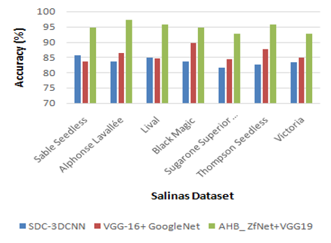
Figures 3 and 4 depict the accuracy evaluation for Salinas and Indian pine dataset. The comparison is done between existing SDC-3DCNN, VGG-16+GoogleNet with the proposed AHB_ZfNet+VGG19. X axis and Y axis show that various class labels and the values obtained in percentage, respectively. When contrasted with existing SDC-3DCNN and v-gg-16+GoogleNet methods achieve 85.2% and 86.4% of accuracy, respectively, while the proposed AHB_ZfNet+VGG19method achieves 98.27% of accuracy for Salinas datasets, which is13.07% and 12.27% better than SDC-3DCNN and VGG-16+GoogleNet. While analyzing Indian pine dataset, SDC-3DCNN and VGG-16+GoogleNet method achieves 86.5% and 87%, while the proposed AHB_ZfNet+VGG19 achieves 98.45% of accuracy, which is 12.15% and 11.45% better than existing methods. Table 2 shows the performance analysis of precision for different methods.
Figure 3. Analysis of accuracy for Salinas’s dataset
Figure 4. Analysis of accuracy for Indian pine dataset
Table 1. Performance analysis of accuracy for different methods
|
|
Salinas Dataset |
Indian Pine Dataset |
|||||
|
Class label |
SDC-3DCNN |
VGG 16+GoogleNet |
AHB_ ZfNet+VGG19 |
Class label |
SDC-3DCNN |
VGG-16+GoogleNet |
AHB_ ZfNet+VGG19 |
|
Sable Seedless |
85.6 |
83.6 |
94.6 |
Autumn Royal |
84.6 |
85.3 |
94.3 |
|
Alphonse Lavallée |
83.7 |
86.4 |
97.3 |
Crimson |
82.6 |
84.6 |
97.8 |
|
Lival |
84.9 |
84.6 |
95.7 |
Itum4 |
87.1 |
85.4 |
96.3 |
|
Black Magic |
83.6 |
89.6 |
94.6 |
Itum5 |
85.6 |
86.4 |
98.5 |
|
Sugarone Superior Seedless |
81.6 |
84.3 |
92.8 |
Itum9 |
87.3 |
86.2 |
92.6 |
|
Thompson Seedless |
82.6 |
87.6 |
95.8 |
Vinyard_untrained |
82.4 |
86.7 |
94.7 |
|
Victoria |
83.4 |
84.9 |
92.6 |
Vinyard_vertical_trellis |
87.3 |
87.9 |
96.8 |
Table 2. Performance analysis of precision for different methods
|
|
Salinas Dataset |
Indian Pine Dataset |
|||||
|
Class label |
SDC-3DCNN |
VGG-16+GoogleNet |
AHB_ZfNet+VGG19 |
Class label |
SDC-3DCNN |
VGG-16+GoogleNet |
AHB_ZfNet+VGG19 |
|
Sable Seedless |
82.6 |
87.4 |
98.3 |
Autumn Royal |
84.6 |
86.5 |
98.6 |
|
Alphonse Lavallée |
84.9 |
86.5 |
97.4 |
Crimson |
87.5 |
89.7 |
98.7 |
|
Lival |
87.3 |
87.2 |
98.5 |
Itum4 |
83.5 |
83.4 |
96.6 |
|
Black Magic |
82.5 |
86.3 |
97.8 |
Itum5 |
84.6 |
87.5 |
97.9 |
|
Sugarone Superior Seedless |
84.6 |
87.9 |
94.7 |
Itum9 |
87.4 |
84.9 |
97.5 |
|
Thompson Seedless |
87.3 |
85.3 |
96.3 |
Vinyard_untrained |
84.2 |
82.6 |
97.8 |
|
Victoria |
85.9 |
84.6 |
94.8 |
Vinyard_vertical_trellis |
86.7 |
84.9 |
98.4 |
Figure 5. Analysis of precision for Salinas’s dataset
Figures 5 and 6 depict the precision evaluation for Salinas and Indian pine dataset. The comparison is done between existing SDC-3DCNN, VGG-16+GoogleNet with the proposed AHB_ZfNet+VGG19. X axis and Y axis show that various class labels and the values obtained in percentage, respectively. When contrasted with existing SDC-3DCNN and v-gg-16+GoogleNet methods achieve 82.1% and 84.3% of precision, respectively, while the proposed AHB_ZfNet+VGG19method achieves 97.67% of precision for Salinas dataset, which is 15.57% and 13.37% better than SDC-3DCNN and VGG-16+GoogleNet. While analyzing Indian pine dataset, SDC-3DCNN and VGG-16+GoogleNet method achieves 84% and 82%, while the proposed AHB_ZfNet+VGG19 achieves 97.1% of precision, which is 13.1% and 15% better than the existing methods. Table 3 shows the performance analysis of recall for different methods.
Figure 6. Analysis of precision for Indian pine dataset
The recall assessment for the Salinas and Indian Pine datasets is shown in Figures 7 and 8. The suggested AHB_ZfNet+VGG19 is compared with the already existing SDC-3DCNN VGG-16+GoogleNet. Different class names and percentage values are shown on the X and Y axes, correspondingly. When contrasted with existing SDC-3DCNN and VGG-16+GoogleNet methods achieve 87.3% and 85.2% of recall, respectively, while the proposed AHB_ZfNet+VGG19 method achieves 97.41% of recall for Salinas datasets, which is 20.11% and 12.21% better than SDC-3DCNN and VGG-16+GoogleNet. While analyzing Indian pine dataset, SDC-3DCNN and VGG-16 16+GoogleNet methods achieves 89% and 86% while the proposed AHB_ZfNet+VGG19 achieves 97.41% of recall, which is 6.5% and 11% better than the existing methods. Table 4 shows the performance analysis of F1_score for different methods.
Figure 7. Analysis of recall for Salinas dataset
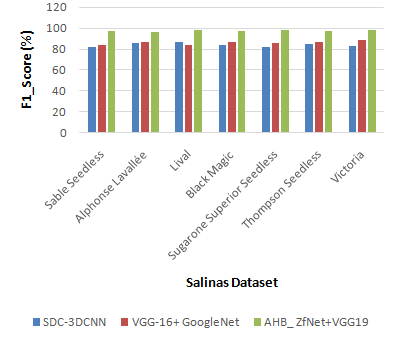
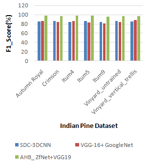
The F1-score analysis for the Salinas and Indian Pine datasets is shown in Figures 9 and 10. The suggested AHB_ZfNet+VGG19 is compared with the already existing SDC-3DCNN VGG-16+GoogleNet. Different class names and percentage values are shown on the X and Y axes, accordingly. When contrasted, existing SDC-3DCNN and VGG-16+GoogleNet methods achieve 83.4% and 83% of F1-scorerespectively, while the proposed AHB_ZfNet+VGG19 method achieves 97.74% of F1-score for Salinas dataset, which is 14.31% and 14.3% better than SDC-3DCNN and VGG-16+GoogleNet. While analyzing Indian pine dataset, SDC-3DCNN and VGG-16+GoogleNet methods achieved 86.4% and 82.4%, while the proposed AHB_ZfNet+VGG19 achieves 97.6% of F1-score, which is 11.2% and 15.2% better than existing methods.
Tables 5 and 6 show the analysis of Salinas’s dataset and Indian pine dataset for the proposed AHB_ZfNet+VGG19.
Figure 8. Analysis of recall for Indian pine dataset
Table 3. Performance analysis of recall for different methods
|
|
Salinas Dataset |
Indian Pine Dataset |
|||||
|
Class label |
SDC-3DCNN |
VGG-16+GoogleNet |
AHB_ZfNet+VGG19 |
Class label |
SDC-3DCNN |
VGG-16+GoogleNet |
AHB_ZfNet+VGG19 |
|
Sable Seedless |
87.4 |
86.4 |
97.45 |
Autumn Royal |
86.4 |
84.6 |
96.53 |
|
Alphonse Lavallée |
89.3 |
87.4 |
96.2 |
Crimson |
84.5 |
87.5 |
97.56 |
|
Lival |
84.4 |
86.5 |
98.4 |
Itum4 |
87.4 |
84.6 |
98.4 |
|
Black Magic |
87.6 |
85.3 |
96.9 |
Itum5 |
82.6 |
87.5 |
97.6 |
|
Sugarone Superior Seedless |
85.1 |
82.6 |
94.8 |
Itum9 |
84.6 |
86.2 |
98.2 |
|
Thompson Seedless |
86.3 |
84.7 |
97.5 |
Vinyard_untrained |
87.4 |
86.5 |
96.8 |
|
Victoria |
84.3 |
84.6 |
96.3 |
Vinyard_vertical_trellis |
89.6 |
86.3 |
94.5 |
Table 4. Performance analysis of F1_score for different methods
|
|
Salinas Dataset |
Indian Pine Dataset |
|||||
|
Class label |
SDC-3DCNN |
VGG-16+GoogleNet |
AHB_ZfNet+VGG19 |
Class label |
SDC-3DCNN |
VGG-16+GoogleNet |
AHB_ZfNet+VGG19 |
|
Sable Seedless |
81.8 |
84.6 |
97.65 |
Autumn Royal |
86.5 |
86.7 |
98.65 |
|
Alphonse Lavallée |
86.4 |
87.4 |
96.58 |
Crimson |
87.3 |
84.9 |
97.74 |
|
Lival |
87.4 |
84.5 |
98.32 |
Itum4 |
84.7 |
87.6 |
98.54 |
|
Black Magic |
84.6 |
87.5 |
97.48 |
Itum5 |
86.9 |
83.5 |
98.78 |
|
Sugarone Superior Seedless |
82.6 |
86.4 |
98.25 |
Itum9 |
84.6 |
81.6 |
96.82 |
|
Thompson Seedless |
84.7 |
87.5 |
97.8 |
Vinyard_untrained |
86.8 |
84.6 |
97.56 |
|
Victoria |
83.5 |
89.4 |
98.4 |
Vinyard_vertical_trellis |
86.4 |
89.7 |
98.23 |
Figure 9. Analysis of F1-score for Salinas dataset
Figure 10. Analysis of F1-score for Indian pine dataset
Table 5. Parametric analysis on Salinas’s dataset for the proposed AHB_ZfNet+VGG19
|
Class label |
Accuracy |
Precision |
Recall |
F1-score |
|
Sable Seedless |
97.3 |
96.7 |
97.6 |
97.6 |
|
Alphonse Lavallée |
99.7 |
97.6 |
98.9 |
97.6 |
|
Lival |
96.8 |
98.5 |
97.4 |
97.6 |
|
Black Magic |
99.6 |
97.6 |
95.8 |
96.8 |
|
Sugarone Superior Seedless |
97.5 |
96.8 |
94.5 |
98.5 |
|
Thompson Seedless |
98.4 |
98.9 |
97.3 |
97.6 |
|
Victoria |
98.6 |
97.6 |
98.5 |
98.5 |
|
Average |
98.27 |
97.67 |
97.41 |
97.74 |
Table 6. Parametric analysis on Indian pine dataset using the proposed AHB_ZfNet+VGG19
|
Class label |
Accuracy |
Precision |
Recall |
F1-score |
|
Autumn Royal |
98.4 |
95.8 |
96.9 |
98.5 |
|
Crimson |
97.6 |
96.7 |
97.8 |
96.7 |
|
Itum4 |
98.9 |
97.6 |
96.8 |
98.7 |
|
Itum5 |
98.5 |
98.1 |
94.9 |
95.9 |
|
Itum9 |
97.9 |
94.9 |
93.4 |
97.5 |
|
Vinyard_untrained |
98.7 |
97.5 |
98.2 |
98.4 |
|
Vinyard_vertical_trellis |
99.2 |
98.5 |
98.9 |
97.8 |
|
Average |
98.45 |
97.1 |
97.41 |
97.6 |
This research demonstrates the potential of hyper spectral remote sensing technology for early detection of viral infections in grapevines, particularly in the case of the newly discovered DNA virus, grapevine vein-clearing virus (GVCV). The study successfully identifies and categorizes infected grapevines during their initial asymptomatic stages, paving the way for timely intervention to prevent disease spread across vineyards. By using hyper spectral photography at the plant level and employing a statistical technique, the research effectively distinguishes between healthy and GVCV-infected grapevines based on their reflectance spectra patterns. The integration of the artificial hummingbird optimization technique aids in feature extraction, ensuring the selection of pertinent features and enhancing overall model classification accuracy. Moreover, the adoption of a nondestructive method to calculate total chlorophyll content in grape leaves provides valuable insights into disease severity assessment. The correlation between chlorophyll concentration and reflectance measurements in specific spectral ranges offers a non-invasive means to gauge disease impact on grapevine health. The hybrid approach utilizing ZfNet+VGG19 for pixel-wise and image-wise classification of disease severity showcases the effectiveness of the proposed methodology in accurately identifying and categorizing GVCV infections. Overall, this research establishes hyper spectral remote sensing as a promising tool for the early detection and monitoring of viral infections in grapevines, providing valuable support for viticulture farmers and researchers in managing disease outbreaks and maintaining crop health. The findings of this study contribute significantly to the field of agricultural diagnostics and offer new avenues for precision farming practices. Continued research in this area may lead to even more advanced and efficient disease detection methods, ultimately benefiting the grapevine industry and promoting sustainable and resilient agriculture.
[1] Sowmyalakshmi, R., Jayasankar, T., PiIllai, V.A., Subramaniyan, K., Pustokhina, I.V., Pustokhin, D.A., Shankar, K. (2021). An optimal classification model for rice plant disease detection. Comput. Mater. Contin, 68: 1751-1767. http://dx.doi.org/10.32604/cmc.2021.016825
[2] Fang, Y., Ramasamy, R.P. (2015). Current and prospective methods for plant disease detection. Biosensors, 5(3): 537-561. https://doi.org/10.3390/bios5030537
[3] Thanarajan, T., Alotaibi, Y., Rajendran, S., Nagappan, K. (2023). Improved wolf swarm optimization with deep-learning-based movement analysis and self-regulated human activity recognition. AIMS Mathematics, 8(5): 12520-12539. https://doi.org/10.3934/math.2023629.
[4] Rumpf, T., Mahlein, A.K., Steiner, U., Oerke, E.C., Dehne, H.W., Plümer, L. (2010). Early detection and classification of plant diseases with support vector machines based on hyperspectral reflectance. Computers and Electronics in Agriculture, 74(1): 91-99. https://doi.org/10.1016/j.compag.2010.06.009
[5] Xie, C., He, Y. (2016). Spectrum and image texture features analysis for early blight disease detection on eggplant leaves. Sensors, 16(5): 676. https://doi.org/10.3390/s16050676
[6] Mahlein, A.K., Rumpf, T., Welke, P., Dehne, H.W., Plümer, L., Steiner, U., Oerke, E.C. (2013). Development of spectral indices for detecting and identifying plant diseases. Remote Sensing of Environment, 128: 21-30. https://doi.org/10.1016/j.rse.2012.09.019
[7] Wahabzada, M., Mahlein, A.K., Bauckhage, C., Steiner, U., Oerke, E.C., Kersting, K. (2016). Plant phenotyping using probabilistic topic models: Uncovering the hyperspectral language of plants. Scientific Reports, 6(1): 22482. https://doi.org/10.1038/srep22482
[8] Rajagopal, S., Thanarajan, T., Alotaibi, Y., Alghamdi, S. (2023). Brain tumor: Hybrid feature extraction based on UNet and 3DCNN. Computer Systems Science & Engineering, 45(2). http://dx.doi.org/10.32604/csse.2023.032488
[9] Adam, E., Mutanga, O., Rugege, D. (2010). Multispectral and hyperspectral remote sensing for identification and mapping of wetland vegetation: A review. Wetlands Ecology and Management, 18: 281-296. https://doi.org/10.1007/s11273-009-9169-z
[10] Narayanan, K.L., Krishnan, R.S., Robinson, Y.H., Julie, E.G., Vimal, S., Saravanan, V., Kaliappan, M. (2022). Banana plant disease classification using hybrid convolutional neural network. Computational Intelligence and Neuroscience, 2022. https://doi.org/10.1155/2022/9153699
[11] Yakkundimath, R., Saunshi, G., Anami, B., Palaiah, S. (2022). Classification of rice diseases using convolutional neural network models. Journal of The Institution of Engineers (India): Series B, 103(4): 1047-1059. https://doi.org/10.1007/s40031-021-00704-4
[12] Cao, Y., Yuan, P., Xu, H., Martínez-Ortega, J.F., Feng, J., Zhai, Z. (2022). Detecting asymptomatic infections of rice bacterial leaf blight using hyperspectral imaging and 3-dimensional convolutional neural network with spectral dilated convolution. Frontiers in Plant Science, 13: 963170. https://doi.org/10.3389/fpls.2022.963170
[13] Nalini, S., Krishnaraj, N., Jayasankar, T., Vinothkumar, K., Britto, A.S.F., Subramaniam, K., Bharatiraja, C. (2021). Paddy leaf disease detection using an optimized deep neural network. Computers, Materials & Continua, 68(1): 1117-1128. http://dx.doi.org/10.32604/cmc.2021.012431
[14] Gui, J., Fei, J., Wu, Z., Fu, X., Diakite, A. (2021). Grading method of soybean mosaic disease based on hyperspectral imaging technology. Information Processing in Agriculture, 8(3): 380-385. https://doi.org/10.1016/j.inpa.2020.10.006
[15] Kukreja, V., Kumar, D. (2021). Automatic classification of wheat rust diseases using deep convolutional neural networks. In 2021 9th International Conference on Reliability, Infocom Technologies and Optimization (Trends and Future Directions) (ICRITO). IEEE, pp. 1-6. https://doi.org/10.1109/ICRITO51393.2021.9596133
[16] Jiang, Q., Wu, G., Tian, C., Li, N., Yang, H., Bai, Y., Zhang, B. (2021). Hyperspectral imaging for early identification of strawberry leaves diseases with machine learning and spectral fingerprint features. Infrared Physics & Technology, 118: 103898. https://doi.org/10.1016/j.infrared.2021.103898
[17] Wang, D., Vinson, R., Holmes, M., Seibel, G., Bechar, A., Nof, S., Luo, Y., Tao, Y. (2018). Early tomato spotted wilt virus detection using hyperspectral imaging technique and outlier removal auxiliary classifier generative adversarial nets (OR-AC-GAN). In 2018 ASABE Annual International Meeting. American Society of Agricultural and Biological Engineers, p. 1. http://dx.doi.org/10.13031/aim.201800660
[18] Alharbi, M., Rajagopal, S.K., Rajendran, S., Alshahrani, M. (2023). Plant disease classification based on ConvLSTM U-Net with fully connected convolutional layers. Traitement du Signal, 40(1): 157. https://doi.org/10.18280/ts.400114
[19] Nguyen, C., Sagan, V., Maimaitiyiming, M., Maimaitijiang, M., Bhadra, S., Kwasniewski, M.T. (2021). Early detection of plant viral disease using hyperspectral imaging and deep learning. Sensors, 21(3): 742. https://doi.org/10.3390/s21030742
[20] Govender, M., Chetty, K., Bulcock, H. (2007). A review of hyperspectral remote sensing and its application in vegetation and water resource studies. Water Sa, 33(2): 145-151. https://doi.org/10.4314/wsa.v33i2.49049
[21] Sawyer, E., Laroche-Pinel, E., Flasco, M., Cooper, M.L., Corrales, B., Fuchs, M., Brillante, L. (2023). Phenotyping grapevine red blotch virus and grapevine leafroll-associated viruses before and after symptom expression through machine-learning analysis of hyperspectral images. Frontiers in Plant Science, 14: 1117869. https://doi.org/10.3389/fpls.2023.1117869
[22] Gu, Q., Sheng, L., Zhang, T., Lu, Y., Zhang, Z., Zheng, K., Hu, H., Zhou, H. (2019). Early detection of tomato spotted wilt virus infection in tobacco using the hyperspectral imaging technique and machine learning algorithms. Computers and Electronics in Agriculture, 167: 105066. https://doi.org/10.1016/j.compag.2019.105066
[23] Soni, A., Dixit, Y., Reis, M.M., Brightwell, G. (2022). Hyperspectral imaging and machine learning in food microbiology: Developments and challenges in detection of bacterial, fungal, and viral contaminants. Comprehensive Reviews in Food Science and Food Safety, 21(4): 3717-3745. https://doi.org/10.1111/1541-4337.12983
[24] Palani, V., Thanarajan, T., Krishnamurthy, A., Rajendran, S. (2023). Deep learning based compression with classification model on CMOS image sensors. Traitement du Signal, 40(3): 1163-1170. https://doi.org/10.18280/ts.400332
[25] Palani, V., Alharbi, M., Alshahrani, M., Rajendran, S. (2023). Pixel optimization using iterative pixel compression algorithm for complementary metal oxide semiconductor image sensors. Traitement du Signal, 40(2): 693-699. https://doi.org/10.18280/ts.400228