Wenli Lei*![]() | Yang Lei
| Yang Lei![]() | Bin Li
| Bin Li![]() | Kun Jia
| Kun Jia![]()
© 2023 IIETA. This article is published by IIETA and is licensed under the CC BY 4.0 license (http://creativecommons.org/licenses/by/4.0/).
OPEN ACCESS
In the realm of face recognition utilising Support Vector Machines (SVM), the adaptivity of the penalty parameter c and the kernel function g is often found lacking, leading to suboptimal recognition rates. To address this issue, an approach harnessing the Sparrow Search Algorithm (SSA) for SVM parameter optimisation has been proposed. Traditional methods such as grid and random search, alongside other swarm intelligence optimisation algorithms like Particle Swarm Algorithm (PSO) and Differential Evolutionary Algorithm (DE), were surpassed by the capabilities of the SSA in numerous applications. Cross-validation (CV) was employed, with the SVM model training recognition accuracy serving as the SSA fitness value. Upon achieving optimal fitness values, the best combination of hyperparameters was ascertained. The overarching aim was to deploy the SSA for global optimisation of SVM's penalty parameters and kernel function, ensuring the derivation of the globally optimal solution for the ultimate classifier model in face recognition tasks. An empirical analysis conducted on the ORL standard face database revealed that the proposed method outperformed the PSO, DE, Gray Wolf Algorithm (GWO), and Enhanced Gray Wolf Algorithm (EGWO), registering an average accuracy of 95.1%. This starkly contrasts with the 81.9% accuracy of the traditional SVM. Such results demonstrate the method's efficacy in enhancing recognition performance, offering a novel avenue to elevate the accuracy of conventional SVM-based face recognition.
support vector machine, sparrow search algorithm, cross-validation, face recognition, principal component analysis
In the modern era of information technology, face recognition technology has garnered significant attention, encompassing diverse technical fields such as image acquisition, feature extraction, and identity verification [1]. Its profound implications are observed within image processing and pattern recognition domains [2]. Since the inception of face recognition algorithms, notable advancements have been made, thereby accentuating its pivotal role in daily life. The challenge of enhancing the accuracy of face recognition to cater to a broader range of application scenarios has been explored by numerous researchers.
Contemporary face recognition techniques are predominantly categorised into three: geometric feature-based methods, template-based methods, and model-based methods [3]. Among these, the template-based method is frequently adopted owing to its simplicity and effectiveness, with Principal Component Analysis (PCA) and Convolutional Neural Networks (CNN) being common techniques [4].
The literature presents a data processing algorithm, the SVM [5, 6]. It is applied for sample classification and recognition, as well as for in-depth data analysis [7]. Rooted in statistical learning theory, SVM employs the principle of structural risk minimisation [8]. Given its inherent attributes, SVM is often utilised for face recognition classification. For instance, an eye pixel feature extraction method centred around Singular Value Decomposition (SVD) and an SVM face recognition method based on feature differences were proposed by Liu and Chen [9]. Though this method mitigates the effects of light and expression, its SVM model was observed to be suboptimal during construction. The singular value decomposition extension algorithm proposed by Fu et al. [10] effectively classifies the algebraic features of face images but encounter challenges with computational complexity and kernel function selection. Liu et al. [11] have explored the amalgamation of the fast PCA algorithm and AdaBoost-based twin support vector machine (TWSVM). While adept at managing high-dimensional data, excessive preprocessing and marginal improvements in recognition accuracy were identified as limitations. Zhang et al. [12] introduced an approach anchored in PCA and SVM, enhancing recognition rates but lacking adaptivity. Furthermore, methods combining CNN with SVM proposed by Feng et al. [13] have shown commendable accuracy but require extensive datasets. Notably, the combination of ant colony algorithms and SVM has been proposed by Sun [14] for multiple feature detection, yet this approach remains computationally intensive. Central to improving SVM's recognition accuracy is enhancing the adaptivity of its penalty parameters and kernel functions, making the optimal selection of hyperparameters paramount.
In 2020, a novel swarm intelligence optimisation algorithm named the SSA was introduced by Xue and Shen [15], inspired by sparrow foraging behaviours. The algorithm mimics the behaviours of sparrows as they search for food and evade predators [16], translating these actions into a mathematical search process, enabling both local and global searches [17]. SSA exhibits superior solution accuracy and faster convergence when compared to PSO and DE. Though SSA combined with SVM has found applications in fields like fault diagnosis [18, 19], image segmentation [20], and model prediction [21, 22], its employment in face recognition remains scarce.
In this study, the dataset from the ORL standard face library is employed. By using PCA, dimensionality of the training and test sets is reduced. In a CV framework, the SSA is harnessed to optimise the penalty parameters and kernel function coefficients of the SVM model, with results indicating enhancements in the model's recognition accuracy and stability.
The ensuing sections of this study are structured as follows: Section 2 elucidates the PCA algorithm and SVM classifier. Section 3 details the design process of optimising the SVM model with SSA. Section 4 outlines the comprehensive process of integrating SSA with SVM for face recognition. Experimental results, discussions, and analyses are presented in Section 5. Conclusions are drawn in Section 6.
PCA, as the term suggests, is primarily designed to handle redundant data, extracting the principal components for retention [23]. From a mathematical perspective, this entails processing sample data via orthogonal transformation to generate a set of linearly uncorrelated variables [24].
As an unsupervised method for dimensionality reduction, PCA aims to project high-dimensional data into a reduced-dimensional space [25]. The objective behind this dimensionality reduction is to lessen the computational effort associated with processing these data [26]. For this transformation to be effective, the original data must be projected in a manner that maximises its variance. Hence, the direction of the dataset variance that achieves maximization serves as the direction of the principal components. A salient feature of PCA's operational principle involves discovering a set of mutually orthogonal axes from the initial space [27]. The goal is to diminish the N original coordinate axes to k efficient axes, thereby accomplishing data dimensionality reduction.
For illustrative purposes, consider a data matrix, X, with dimensions (m×n), representative of m data and n features. If the foremost principal component after mapping is labelled Xproject, and the direction of projection is denoted by u, which serves as a unit direction vector, the representation becomes uTu=1.
The variance of the data post-mapping is articulated as:
$\operatorname{Var}\left( {{\text{X}}_{\text{project }}} \right)=\frac{1}{m}\sum\limits_{i=1}^{m}{{{\left( {{x}^{{{(i)}^{T}}}}u \right)}^{2}}}$ (1)
The equation for computing the mean of the sample matrix is given by:
$\mu =\frac{1}{m}\sum\limits_{i=1}^{m}{{{x}^{(i)}}}$ (2)
From Eq. (1), the covariance matrix of the sample can be deduced as:
$\text{C}=\frac{1}{m}\sum\limits_{i=1}^{m}{{{x}^{(i)}}}{{x}^{{{(i)}^{T}}}}$ (3)
The overarching goal of PCA is to condense high-dimensional data into a specified k-dimension. The implementation follows these steps:
Input of the data: the original data is restructured into an m-row and n-column matrix X by rows; k is the specified number of dimensions.
Upon completion of data processing, the resultant product is a matrix characterised by eigenvectors of reduced dimensions, comprising k columns. The procedures executed to achieve this output are delineated below:
1) The input data were configured into a matrix as previously elucidated, and specific values corresponding to each feature were ascertained.
2) The data sample matrix was subjected to a zero-meaning process in line with Eqs. (1) and (2), from which variance was deduced.
3) Adhering to Eq. (3), the covariance matrix was derived.
4) Eigenvalues, together with their affiliated eigenvectors, were extracted from the aforementioned covariance matrix.
5) The eigenvectors derived in step 4 were systematically organised into a matrix. The principal k columns of this formed matrix were then extracted to compose a novel matrix, denoted as Q.
6) Employing the relation Y=XQ, the data were transformed, facilitating a dimensionality reduction from N dimensions to the specified k dimensions.
3.1 SSA
In parallel to the aforementioned procedures, the SSA, a heuristic method inspired by the natural behaviours of foraging sparrows and their evasion of predators, was integrated into the study. This algorithm is comprised of three distinct sparrow types: discoverers, joiners, and vigilantes [28]. Each plays a unique role, culminating in a comprehensive foraging system. When these three sparrows synergise, the optimal solution, analogous to evading predators whilst locating sustenance, is ascertained.
Discoverers are principally tasked with offering the sparrow population both a direction and location for foraging. Joiners, on the other hand, optimise foraging by incessantly observing the actions of the discoverers, thus enhancing the population's efficiency. Vigilantes maintain a watchful eye for potential threats, signaling imminent dangers to ensure the flock remains unthreatened during their foraging. Equations detailing the position updates for each sparrow type are expounded below.
The discoverer location update formula is as follows:
${{X}_{i,j}}(t+1)=\left\{ \begin{array}{*{35}{l}} {{X}_{i,j}}(t){{e}^{\left( -\frac{i}{\alpha T} \right)}}, & R<ST \\ {{X}_{i,j}}(t)+Q\cdot L, & R\ge ST \\\end{array} \right.$ (4)
where, R symbolizes the warning value while ST signifies the safety value.
The joiner location is updated using the following formula:
${{X}_{i,j}}(t+1)=\left\{ \begin{matrix} Q{{e}^{\left( \frac{{{X}_{\omega }}(t)-{{X}_{i,j}}(t)}{{{i}^{2}}} \right)}}, & i>\frac{n}{2} \\ {{X}_{p}}(t+1)+\left| {{X}_{i,j}}(t)-{{X}_{p}}(t+1) \right|{{A}^{+}}L, & i\le \frac{n}{2} \\\end{matrix} \right.$ (5)
where, the departure from the current suboptimal foraging location is instigated when $i>\frac{n}{2}$. Conversely, optimal foraging sites are pursued in close proximity to the discoverer when $i \leq \frac{n}{2}$.
The location of the vigilantes is updated as follows:
${{X}_{i,j}}(t+1)=\left\{ \begin{array}{*{35}{l}} {{X}_{B}}(t)+\beta \left| {{X}_{i,j}}(t)-{{X}_{B}}(t) \right|, & {{f}_{i}}>{{f}_{g}} \\ {{X}_{i,j}}(t)+K\left( \frac{\left| {{X}_{i,j}}(t)-{{X}_{\omega }}(t) \right|}{\left( {{f}_{i}}-{{f}_{w}} \right)+\varepsilon } \right), & {{f}_{i}}={{f}_{g}} \\\end{array} \right.$ (6)
where, fi represents the extant adaptational value of an individual sparrow, fg denotes the globally optimal adaptation value, and fw stands for the globally least optimal adaptation value.
3.2 SVM
The SVM stands as a rigorously researched classification algorithm. Predominantly utilised for data classification and regression challenges, its core concept is centred on sample classification through the construction of an optimal classification hyperplane [29]. This goal mandates the establishment of a constrained optimisation problem, the resolution of which yields the desired classifier [30]. A visual representation of this optimal classification hyperplane is presented in Figure 1.
Figure 1. Schematic representation of SVM classification
Upon examination of Figure 1, it becomes evident that the optimal solution sought by the SVM is realised when γ is maximised. Thus, the endeavour to identify the optimal hyperplane can be articulated as a quadratic programming challenge, exemplified by:
$\left\{ \begin{matrix} \min \frac{1}{2}\|w{{\|}^{2}} \\ {{y}^{i}}\left( {{w}^{T}}\Phi \left( {{x}_{i}} \right)+b \right)\ge 1,i=1,2, L,n \\\end{matrix} \right.$ (7)
To mitigate the risk of overfitting, the introduction of a relaxation factor δ is necessitated. Consequently, every sample is associated with a relaxation variable, leading to an extended version of Eq. (7):
$\left\{ \begin{matrix} \min \frac{1}{2}\|w{{\|}^{2}}+c\sum\limits_{i=1}^{n}{{{\delta }_{i}}} \\ {{y}^{i}}\left( {{w}^{T}}\Phi \left( {{x}_{i}} \right)+b \right)\ge 1-{{\delta }_{i}} \\\end{matrix} \right.$ (8)
where, c serves as the penalty parameter. A higher c value signifies a stringent classification, while a lower value implies a more relaxed classification, accommodating potential classification losses. The transformation technique, denoted by Φ(x), is referred to as kernel function transformation. For the purposes of this study, the Radial Basis Function (RBF) is adopted as the SVM's kernel function, defined as:
$K\left( x,{{x}^{\prime }} \right)=\exp \left( -\frac{{{\left\| x-{{x}^{\prime }} \right\|}^{2}}}{2{{\sigma }^{2}}} \right)$ (9)
where, σ represents the kernel function parameter. The magnitude of σ has a direct bearing on the SVM classifier's efficacy. In essence, the judicious selection of penalty and kernel function parameters is imperative for optimal classifier performance.
3.3 SSA-based optimization of SVM hyperparameters
Given the inherent variability of SVM model training sets and the significant uncertainty associated with the penalty parameter c and kernel function parameter g (σ in SVM), the resultant performance of the SVM is substantially influenced by these factors [31]. Conventionally, SVM parameters are reliant on empirical values, with typical settings being c as 2 and g as (1/k), where k represents the designated dimension post-PCA dimension reduction. However, such empirical methodologies might render the SVM susceptible to local optima and potential inconsistencies in recognition outcomes.
To enhance SVM's predictive precision and to negate the risk of local optima, the SSA is employed to fine-tune the pivotal parameters c and g, grounded in the principle of CV. Post-CV comparative results, acknowledged for their reliability, effectively counter data overfitting and inform the setting of SVM parameters, thereby elevating the SVM's ultimate accuracy.
The adopted approach entails the arbitrary division of the training set into n identical data subsets. (n-1) of these subsets are employed for training, culminating in an augmented SVM training set, while the residual subset is harnessed to validate the training model's accuracy. This iterative process continues until each subset has undergone CV once. The apex recognition rate from all validation outcomes serves as the SSA's fitness value. Based on the fitness value acquired, SSA undertakes an iterative optimisation search, filtering out extraneous variables, culminating in the identification of the globally optimal penalty parameter c and kernel function parameter g.
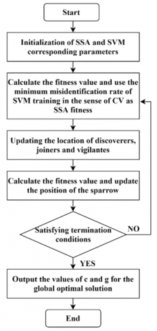
Figure 2 illustrates the fundamental process for the SSA-based optimisation of SVM's key parameters.
The specific procedural steps are delineated as:
Step 1: Initialisation of the sparrow flock's location and fitness values occurs, followed by the demarcation of the boundary values for the parameters under SSA's purview.
Step 2: Variables transcending the boundaries, established in Step 1, are discarded, and a fresh fitness value is computed.
Step 3: Discoverer locations undergo updates based on vigilante and joiner locations. Subsequently, the optimal fitness value is identified. In instances where superior fitness values are detected, locations are updated accordingly.
Step 4: Discoverer, joiner, and vigilante locations are subject to updates.
Step 5: The optimisation process culminates either when the fitness value reaches its zenith and further enhancements are unattainable, or when the iteration count achieves its predetermined limit. Failing that, a return to Step 2 is effected, instigating a new optimisation cycle.
Step 6: The optimal values of parameters c and g are outputted, signalling the conclusion of the global optimisation search process.
Figure 2. Workflow for SVM hyperparameters optimised through SSA
3.4 SVM face recognition optimised through SSA
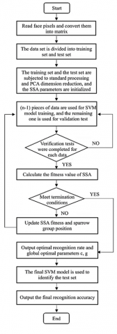
Optimising the accuracy of face recognition can be achieved by determining the optimal parameters, c and g, for SVM via SSA. Subsequent application of these parameters to SVM boosts face classification recognition accuracy. For robustness, SSA parameter configurations were set following multiple simulation tests: the population was set at 20, with a maximum iteration of 50, an alert threshold of 0.8, and a 20% allocation for discoverers. The specific methodology is depicted in Figure 3.
Figure 3. SVM face recognition process optimised through SSA
The specific implementation steps are as follows:
Step 1: Data extraction and labelling. Grayscale values of the facial representations in the dataset were extracted, forming an N×M matrix, where N represents the aggregate count of facial images, while M symbolises the dimensionality of individual image features. Concurrently, the dataset underwent labelling.
Step 2: Data partitioning. The dataset was bifurcated, with test_size established at 0.5, allocating half for testing and the remaining for training purposes.
Step 3: Normalisation of training data. The training dataset was normalised, leading to rule generation. These rules were subsequently applied to the test set during its normalisation process.
Step 4: PCA implementation. The PCA method was applied to reduce the dimensionality of the standardised training data. A regulation based on the training set was produced, subsequently applied to the test set's downsizing.
Step 5: Training data replication and parameter initialization. Post-PCA, the dataset underwent segmentation into n segments. The SVM's kernel function pathway was defined by the RBF kernel. Correspondingly, initial parameters for SSA were defined.
Step 6: Training and validation. Training data was stochastically subdivided into n segments. (n-1) segments were employed to train the SVM model, while the remainder served for SVM validation. This process iterated until every data segment underwent validation.
Step 7: Validation completion check. An assessment was conducted to ascertain if every data subset had been subjected to validation. If validation was complete, the next step ensued; otherwise, the process reverted to step 6.
Step 8: SSA fitness value determination. The apex recognition rate from all validations was designated as SSA's fitness value.
Step 9: Termination criteria check. An evaluation determined if the SSA's fitness value satisfied termination conditions. If met, the utmost recognition accuracy was presented as the final SVM training accuracy, accompanied by the revelation of the optimal values for c and g. Failing satisfaction, the process continued to step 10.
Step 10: Fitness value update and global search. Drawing from step 8, the fitness values of SSA and the respective positions of discoverer, joiner, and vigilante sparrows were updated. The methodology reverted to step 6, continuously seeking SVM parameter optimal solutions through SSA's global search.
Step 11: Global optimal position determination. Completion of all stages resulted in the identification of the global optimal position, yielding the final optimal parameters.
Step 12: Final model testing. With the acquisition of the optimal parameters, the final model was utilised to predict the test set, culminating in the computation of the final accuracy metric.
3.5 Experiment specific process and results
3.5.1 Experimental environment and data pre-processing
The experiment was conducted using an Inter i5-7300 2.50GHz system with a configuration of 8GB RAM, 64-bit OS, Win10. The development environment incorporated both Pycharm2021 and Anaconda3 with Python 3.7. Data were sourced from the ORL standard face database, which comprises 40 distinct faces, with each having 10 different poses, resulting in a total of 400 images of 112×92 pixels each.
Considering the extensive fluctuation observed in the pixel grey values, preprocessing was deemed necessary to make the data suitable for SVM training. The data were then normalized to facilitate subsequent PCA dimensionality reduction. Upon segmenting the dataset into training and test sets, normalization rules applied to the training set were extended to the test set. Dimensionality reduction using PCA was then performed on the pre-processed training set, with the training set rules again applied to the test set.
SSA parameter initialization was undertaken with the fitness value initialized, optimizing for a minimum c value of 0.1 and a maximum of 10, while for g, the range was established between 2-5 and 16. 20% of the total population size was set as the population size of discoverers. An environment safety threshold was established at 0.8; any value below was deemed safe, while values equal to or surpassing this threshold signified potential risks affecting the foraging behaviour of the population. The experiment was set with a maximum iteration of 50 and a population number of 20.
For the SVM, the RBF Gaussian kernel function was employed, with c and g parameters adopting values of 2 and (1/k) in the empirical case. k represents the number of dimensions determined by the PCA downscaling. A CV of 5 was employed, and according to data separation in the ORL dataset, a test size of 0.5 was used. That is, five random images of each individual were selected, constituting the training data set, while the residual five images were designated as the test data set.
3.5.2 Analysis of experimental results
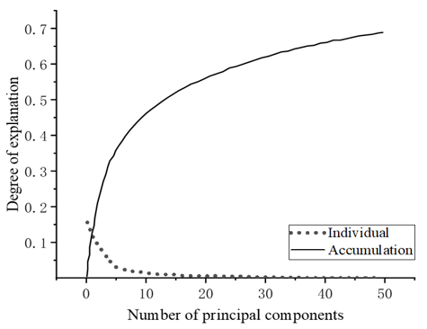
Post-dimensionality reduction by PCA, the degree to which the original data was explained in the specified dimensions was evaluated using the ORL face library. As illustrated in Figure 4, which represents the original data restored in the initial 50 dimensions, a declining trend was observed in the degree of explanation, settling at 18% for the first dimension but diminishing to less than 1% by the 50th dimension. However, the accumulated explanatory degree reached approximately 70% for these 50 dimensions.
Figure 4. Degree of original data restored in the first 50 dimensions
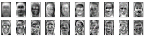
Figure 5. 20 feature faces extracted by PCA
Subsequent to this, the dataset was subjected to dimensionality reduction using PCA, scaling it down to 20 dimensions. The resultant feature faces are illustrated in Figure 5, affirming that these 20 characteristic facial representations encompass the salient features of the entire data set. Consequently, all 400 images from the ORL library could be reconstructed via linear combinations of these characteristic surfaces.
Upon analysing Figure 5, a notable observation is the minimal variation in the background of ORL library facial images post-grayscale processing. This uniformity manifests as a darker background in the feature faces extracted by PCA, with the exception of the facial outline. A closer scrutiny of the first 20 principal component feature faces reveals regions of higher grayscale values - particularly around the eyes, eyebrows, and lips. This indicates greater variance in the original images in these zones, denoting their significance in facial identification. It can thus be inferred that the feature faces procured via PCA have retained essential characteristics while dispensing superfluous information.
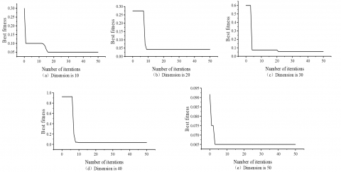
Further, the optimal fitness curves of the first 50 principal components post SSA optimization for SVM are depicted in Figure 6. The penalty parameter c and kernel function coefficients g of the SVM were fine-tuned using SSA, and the ensuing face recognition outcomes corresponding to the optimal global parameters are documented in Table 1. For comparative analysis, the recognition results when c and g were adopted as empirical values are provided in Table 2.
As depicted in Figure 6, convergence curves corresponding to principal components spanning from 10 to 50 dimensions were presented. It was observed that an optimal adaptation value can be ascertained within an iteration count of 50. A comparative analysis of Tables 1 and 2 revealed the superior performance of the SSA-optimized SVM. Specifically, the accuracy surpassed 90% when optimized, whereas the unoptimized variant consistently recorded accuracy levels below 90%, with its zenith at 85.5% and nadir at 73% in the 10th dimension. In stark contrast, SSA optimization delivered an impressive accuracy of 95%.
A deeper examination of recognition results across the first 50 dimensions elucidated that post-SSA optimization, not only was the recognition accuracy elevated, but the results also displayed greater stability. Conversely, the unoptimized SVM exhibited fluctuating recognition outcomes, particularly within the dimension range of 10 to 20, underscoring the instability inherent to its results. Such observations buttress the notion that parameters refined via SSA render enhanced guidance, thereby circumventing SVM's local optima. Consequently, the SVM model, when subjected to global optimal parameter identification through SSA, demonstrated exemplary performance.
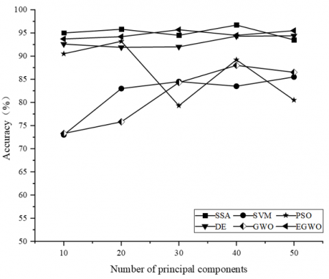
To further corroborate the efficacy of the methodology delineated in this study, the mean and standard deviation of recognition accuracy corresponding to algorithms such as KTWSVM and ABKTWSVM, as employed by Liu et al. [11], were juxtaposed against the classical SVM algorithms. This comparison is catalogued in Table 3. For ensuring equitable assessment, data spanning the first 50 dimensions were chosen. Additionally, optimization strategies such as PSO, DE, GWO, and EGWO [32] were incorporated into this experimental setup. Their respective recognition accuracy outcomes are chronicled in Table 4, and a graphical representation of accuracy trajectories across diverse optimization frameworks, juxtaposed with classical SVM algorithms, can be gleaned from Figure 7.
Table 1. Face image recognition results with SVM parameter optimisation through SSA
|
Dimensionality |
Optimised c |
Optimised g |
Accuracy /% |
|
10 |
2.2438 |
0.9281 |
95.0 |
|
20 |
0.8668 |
0.2100 |
95.8 |
|
30 |
1.7812 |
0.4606 |
94.5 |
|
40 |
1.2684 |
0.0700 |
96.7 |
|
50 |
1.1068 |
0.0408 |
93.5 |
Table 2. Face recognition results without SVM parameter optimisation through SSA
|
Dimensionality |
Experience Value c |
Experience Value g |
Accuracy /% |
|
10 |
2 |
1/10 |
73.0 |
|
20 |
2 |
1/20 |
83.0 |
|
30 |
2 |
1/30 |
84.5 |
|
40 |
2 |
1/40 |
83.5 |
|
50 |
2 |
1/50 |
85.5 |
Figure 6. Fitness convergence curve of the first 50 dimensions
Table 3. Comparison of average and standard deviation of recognition accuracy of different algorithms
|
Algorithm |
Average Value |
Standard Deviation |
|
PCA+SVM |
81.900 |
4.532 |
|
KTWSVM |
88.500 |
2.449 |
|
ABKTWSVM |
89.986 |
2.690 |
|
SSA+PCA+SVM |
95.100 |
1.094 |
Table 4. Accuracy of face recognition with different optimisation algorithms (%)
|
Dimensionality |
PSO |
DE 1 |
GWO |
EGWO 1 |
SSA |
|
10 |
90.5 |
92.6 |
73.3 |
93.7 |
95.0 |
|
20 |
93.2 |
91.9 |
75.8 |
94.2 |
95.8 |
|
30 |
79.3 |
92.0 |
84.3 |
95.7 |
94.5 |
|
40 |
89.2 |
94.3 |
88.0 |
94.5 |
96.7 |
|
50 |
80.5 |
94.4 |
86.5 |
95.5 |
93.5 |
1 The data in this column are derived from the literature [32].
Table 5. Comparison of parameter means and standard deviations for different optimisation algorithms
|
Algorithm |
Parameter c |
Parameter g |
||
|
Average |
SD2 |
Average |
SD2 |
|
|
PSO |
5.034 |
1.676 |
0.523 |
0.161 |
|
DE |
84.254 |
24.689 |
0.066 |
0.140 |
|
GWO |
6.799 |
2.422 |
0.233 |
0.285 |
|
EGWO |
20.729 |
24.415 |
0.159 |
0.120 |
|
SSA |
1.474 |
0.235 |
0.230 |
0.150 |
2 SD is expressed as an abbreviated form of standard deviation.
Figure 7. Recognition accuracy of different algorithms
As depicted in Table 3, significant variations in the recognition accuracy among different algorithms are observed. When subjected to SSA optimisation, an average SVM accuracy of 95.1% was achieved, contrasted against an average SVM accuracy of 81.9% without optimisation. The KTWSVM and ABKTWSVM, when compared, displayed average accuracies of 88.5% and 89.986% respectively. Additionally, the standard deviation of accuracy for the SSA was found to be 1.094, notably lower than its counterparts. These findings suggest that not only does SSA optimisation enhance the accuracy of SVM, but the resultant recognition outcomes are also more closely clustered around the mean, exhibiting reduced volatility and resilience against settling in local optima.
Upon examining both Table 4 and Figure 7, it was discerned that the SSA exhibited commendable performance even with a limited number of iterations, consistently registering recognition rates exceeding 90%. In contrast, PSO was noted to experience premature convergence, leading to a reduction in recognition rates as dimensionalities increased. GWO's performance was suboptimal, attributed to a minimal iteration count. While both EGWO and DE achieved overall accuracies surpassing 90%, with EGWO slightly outpacing the algorithms proposed in referenced literature [32] at certain dimensions, their accuracies (averaging 94.7% and 93% respectively) remained inferior to SSA's 95.1%. These outcomes imply not only the superiority of SSA in augmenting SVM performance but also its ability to ensure optimal recognition accuracy with minimal iterations.
Furthermore, in a study where images were randomly downsampled to 30 dimensions, 20 independent trials were conducted to assess algorithm stability using the mean and standard deviation of the penalty parameter c and the kernel function parameter g. Table 5 offers a comparative insight into these parameters for various optimisation algorithms.
From the data presented in Table 5, it was determined that the average value of parameter c optimised via SSA was considerably lower than that optimised by other algorithms, potentially minimising SVM's susceptibility to overfitting. Concurrently, the standard deviation associated with the c parameter for SSA was also observed to be smaller than other algorithms, indicative of a narrow fluctuation range and heightened stability. Although the g parameter for SSA exceeded that of EGWO and DE, the values for parameter c of EGWO and DE displayed significant volatility. In comparison, the parameters optimised by SSA appeared to offer more consistent guidance.
In efforts to augment the face recognition accuracy of SVM, an algorithm predicated on SSA-optimised SVM was introduced. Through rigorous evaluation, it was discerned that under the CV paradigm, an average accuracy rate of 95.1% was achieved upon employing SSA for SVM parameter optimisation. This level of accuracy surpassed that attained by other optimisation algorithms. Furthermore, superior advantages in terms of SVM performance and stability were observed when parameters were optimised using SSA. Future endeavours should seek to address the prolonged duration associated with PCA feature extraction. Additionally, refining the SSA algorithm to strike a harmonious balance between local and global searches, thereby enhancing its prowess in pinpointing optimal solutions, warrants exploration.
This work was supported by the Shaanxi Provincial Key Laboratory for Intelligent Processing of Big Data in Energy (Grant No.: IPBED11, IPBED1), partially funded by Yan'an University Doctoral Research Initiation Project (Grant No.: YDBK2018-39) and Yan'an University Graduate Education Innovation Program Project (Grant No.: YCX2021070, YCX2023032, YCX2023033), also supported by the Emergency Research Project on Epidemic Prevention and Control (Grant No.: ydfk007, ydfk062, ydfk060, ydfk064), the Special Research Project on Epidemic Prevention and Control and Economic and Social Development (Grant No.: YCX2022075, YCX2022079) of Yan'an University, and the "14th Five Year Plan Medium and Long Term Major Scientific Research Project" (Grant No.: 2021ZCQ015) of Yan'an University.
[1] Fatima, M., Ghauri, S.A., Mohammad, N.B., Adeel, H., Sarfraz, M. (2022). Machine learning for masked face recognition in COVID-19 pandemic situation. Mathematical Modelling of Engineering Problems, 9(1): 283-289. https://doi.org/10.18280/mmep.090135
[2] Huang, S.F., Tang, L.J. (2022). Overview of face recognition technology. China High Technology, 8: 10-11.
[3] Maulenov, K., Kudubayeva, S., Razakhova, B. (2023). Modern problems of face recognition systems and ways of solving them. Revue d'Intelligence Artificielle, 37(1): 209-214. https://doi.org/10.18280/ria.370126
[4] Kanawade, B., Surve, J., Khonde, S.R., Khedkar, S.P., Pansare, J.R., Patil, B., Pisal, S., Deshpande, A. (2023). Automated human recognition in surveillance systems: An ensemble learning approach for enhanced face recognition. Ingénierie des Systèmes d’Information, 28(4): 877-885. https://doi.org/10.18280/isi.280409
[5] Vapnik, V.N. (1999). An overview of statistical learning theory. IEEE Transactions on Neural Networks, 10(5): 988-999. https://doi.org/10.1109/72.788640
[6] Suykens, J.A., Vandewalle, J. (1999). Least squares support vector machine classifiers. Neural Processing Letters, 9: 293-300. https://doi.org/10.1023/A:1018628609742
[7] Wu, J., Yang, H. (2015). Linear regression-based efficient SVM learning for large-scale classification. IEEE Transactions on Neural Networks and Learning Systems, 26(10): 2357-2369. https://doi.org/10.1109/TNNLS.2014.2382123
[8] Zhu, C.Y., Zhang, C., Guan, J.H. (2023). An airspace traffic situation identification method based on improved support vector machine. Transportation Information and Safety, 41(2): 76-85. https://doi.org/10.3963/j.jssn.1674-4861.2023.02.008
[9] Liu, X.D., Chen, Z.Q. (2004). Research on face recognition technology. Computer Research and Development, 7: 1074-1080.
[10] Fu, H.H., Zhao, P.F., Hou, Y.W. (2018). Face recognition algorithm based on least squares support vector machine. Journal of Changchun Engineering College (Natural Science Edition), 19(1): 97-99.
[11] Liu, J.M., Zhang, J., Lei, J. (2020). Adaboost-based face recognition method for twinned support vector machines. Sensors and Microsystems, 39(7): 51-53, 57.
[12] Zhang, Y., Zhang, F., Guo, L. (2021). Face recognition based on principal component analysis and support vector machine algorithms. In 2021 40th Chinese Control Conference (CCC), pp. 7452-7456. https://doi.org/10.23919/CCC52363.2021.9550727
[13] Feng, Y.B., Lu, Y.Q., Zhong, W.B. (2021). Design and implementation of face recognition system based on CNN and SVM. Computer and Digital Engineering, 49(2): 378-382, 420.
[14] Sun, S.S. (2016). Ant colony algorithm optimized support vector machine for face recognition. Modern Electronic Technology, 39(21): 92-94, 98.
[15] Xue, J.K., Shen, B. (2020). A novel swarm intelligence optimization approach: Sparrow search algorithm. Systems Science & Control Engineering, 8(1): 22-34. https://doi.org/10.1080/21642583.2019.1708830
[16] Wu, Z.Q., Wang, B. (2021). An ensemble neural network based on variational mode decomposition and an improved sparrow search algorithm for wind and solar power forecasting. IEEE Access, 9: 166709-166719. https://doi.org/10.1109/ACCESS.2021.3136387
[17] Li, B.Y., Zhang, F., Peng, X. (2022). K-means+SSA-Elman network visible light indoor position perception algorithm. Applied Optics, 43(3): 453-459.
[18] Chen, X., Xiao, M.Q., Sun, Y. (2021). Fiber optic gyro fault diagnosis based on improved sparrow search algorithm and support vector machine. Journal of Air Force Engineering University (Natural Science Edition), 22(3): 33-40.
[19] Ma, C.P., Li, M.H., Kong, Q.L. (2021). Optimized support vector machine based on sparrow search algorithm for rolling bearing fault diagnosis. Science, Technology and Engineering, 21(10): 4025-4029.
[20] Yan, M., Xia, Y.H., Gu, J.L. (2023). Segmentation of ancient architectural color paintings based on multi-strategy improved sparrow search algorithm optimized SVM. Journal of Southwest Normal University (Natural Science Edition), 48(7): 80-88.
[21] Wang, H.F., Xing, H.Y., Chen, M. (2022). SSA-SVM based small signal detection method in sea clutter background. Journal of Electronic Measurement and Instrumentation, 36(4): 24-31.
[22] Yang, L., Wei, J., Xu, Z.F. (2022). Landslide displacement prediction based on smoothing a priori method-sparrow search algorithm-support vector machine regression model-taking Bazimen and Baishui River landslides in Three Gorges Reservoir Area as an example. Journal of Earth Science and Environment, 44(6): 1096-1110.
[23] Li, Y., Yang, H.T., Kong, Z. (2022). A review of pixel-level infrared and visible light image fusion methods. Computer Engineering and Applications, 58(14): 40-50.
[24] Guo, L., Zhou, W.J., Gao, S.W. (2021). Research on face recognition technology based on PCA algorithm. Modern Information Technology, 5(5): 108-112, 117.
[25] Geng, M., Zhang, H.C., Kang, L.Q. (2023). Prediction of bearing remaining life of process equipment based on principal component analysis and random forest regression model. Urban Rail Transit Research, 26(4): 12-16.
[26] Wang, Y.D., Lv, W.D., Hu, C.C. (2022). Research on face image recognition based on PCA, LDA and LR fusion algorithms. Science and Technology Innovation, 22: 72-75.
[27] Yan, L.J., Zhang, Y.H. (2022). Fast face recognition algorithm based on image gradient compensation. Computer System Application, 29(12): 194-201.
[28] Hu, H.Z., Qin, C., Guan, F., Zhang, H.B., An, S.J. (2021). Tool wear identification based on sparrow search algorithm optimization support vector machine. Science, Technology and Engineering, 21(25): 10755-10761.
[29] Xue, Y., Dou, D., Yang, J. (2020). Multi-fault diagnosis of rotating machinery based on deep convolution neural network and support vector machine. Measurement, 156: 1-7. https://doi.org/10.1016/j.measurement.2020.107571
[30] Feng, Z.L., Xiao, H.Q., Ren, W.F. (2023). Transformer fault diagnosis by seagull optimization support vector machine based on principal component analysis. China Test, 49(2): 99-105.
[31] Liao, Z.Y., Wang, Y.T., Xie, X.L. (2017). Support vector machine face recognition based on particle swarm optimization. Computer Engineering, 43(12): 248-254.
[32] Feng, J., Pei, D., Wang, W. (2019). Optimized support vector machine based on improved grey wolf algorithm for face recognition. Computer Engineering and Science, 41(6): 1057-1063.