Fahad M. Alshagathrh*![]() | Saleh Musleh
| Saleh Musleh![]() | Mahmood Alzubaidi
| Mahmood Alzubaidi![]() | Jens Schneider
| Jens Schneider![]() | Mowafa S. Househ
| Mowafa S. Househ![]()
© 2023 IIETA. This article is published by IIETA and is licensed under the CC BY 4.0 license (http://creativecommons.org/licenses/by/4.0/).
OPEN ACCESS
Introduction: Artificial Intelligence (AI) is widely used in medical studies to interpret imaging data and improve the efficiency of healthcare professionals. Nonalcoholic fatty liver disease (NAFLD) is a common liver abnormality associated with an increased risk of hepatic cirrhosis, hepatocellular carcinoma, and cardiovascular morbidity and mortality. This study explores the use of AI for automated detection of hepatic steatosis in ultrasound images. Background: Ultrasound is a non-invasive, cost-effective, and widely available method for hepatic steatosis screening. However, its accuracy depends on the operator's expertise, necessitating automated methods to enhance diagnostic accuracy. AI, particularly Convolutional Neural Network (CNN) models, can provide accurate and efficient analysis of ultrasound images, enabling automated detection, improving diagnostic accuracy, and facilitating real-time analysis. Problem Statement: This study aims to evaluate deep learning methods for binary classification of hepatic steatosis using ultrasound images. Methodology: Open-source data is used to prepare three groups (A, B, C) of ultrasound images in different sizes. Images are augmented using seven pre-processing approaches (resizing, flipping, rotating, zooming, contrasting, brightening, and wrapping) to increase image variations. Seven CNN classifiers (EfficientNet-B0, ResNet34, AlexNet, DenseNet121, ResNet18, ResNet50, and MobileNet_v2) are evaluated using stratified 10-fold cross-validation. Six metrics (accuracy, sensitivity, specificity, precision, F1 score, and MCC) are employed, and the best-performing fold epochs are selected. Experiments and Results: The study evaluates seven models, finding EfficientNet-B0, ResNet34, DenseNet121, and AlexNet to perform well in groups A and B. EfficientNet-B0 shows the best overall performance. It achieves high scores for all six metrics, with accuracy rates of 98.9%, 98.4%, and 96.3% in groups A, B, and C, respectively. Discussion and Conclusion: EfficientNet-B0, ResNet34, and DenseNet121 exhibit potential for classifying fatty liver ultrasound images. EfficientNet-B0 demonstrates the best average accuracy, specificity, and sensitivity, although more training data is needed for generalization. Complete and medium-sized images are preferred for classification. Further evaluation of other classifiers is necessary to determine the best model.
non-alcoholic fatty liver, hepatic steatosis, EfficientNet-B0, ResNet34, image classification, deep learning, binary classification, convolutional neural network, image transformations, ultrasound images
Artificial intelligence (AI) and its methodologies have become increasingly important in medicine with the emergence of Big Data. Although the concept of AI was first proposed in the 1950s [1], recent technological advancements have resulted in breakthroughs. AI refers to computer programs that attempt to replicate human cognitive functions such as learning and problem-solving. Machine learning (ML), developed as a subfield of AI, initially processed data to construct algorithms capable of detecting patterns of behavior from which predictive models could be built. Numerous studies in the field of medicine have utilized a variety of ML approaches, including support vector machines (SVMs), artificial neural networks (ANNs), and classification and regression trees [2]. However, over the past decade, technological advancements have resulted in the emergence of deep learning (DL) as a new machine learning (ML) model for developing multi-layered neural network algorithms. Techniques such as convolutional neural networks (CNN), a multilayer of ANNs that has proven to be extremely useful for image analysis [3, 4].
AI's potential to revolutionize healthcare is increasingly evident as it analyzes vast amounts of medical data [5]. In medicine, AI has been frequently used in fields that require the interpretation of imaging data, such as ultrasonography [6], radiology [7], dermatology [8], pathology [9], and ophthalmology [10]. The emergence of AI may address healthcare professionals' quest for increased efficacy and efficiency in clinical work. One area of medicine where AI has been applied is in diagnosing and monitoring nonalcoholic fatty liver disease (NAFLD), a common liver abnormality found in a substantial percentage of obese people [11]. NAFLD is described as fat build-up in more than 5% of liver cells, and it is linked to an increased risk of hepatic cirrhosis and hepatocellular carcinoma, as well as increased cardiovascular morbidity and death in afflicted individuals [12, 13].
The reference standard for direct liver steatosis measurement in hepatic tissue samples is liver biopsy [14]. However, the biopsy is an expensive and intrusive process with a significant risk of major consequences, such as discomfort, hemorrhage, and, in rare circumstances, death [14]. As a result, liver biopsy is not regarded as a straightforward or ideal method of assessing and monitoring the progression of common liver illnesses. Therefore, non-invasive liver imaging technologies such as computed tomography (CT), magnetic resonance imaging (MRI), and ultrasound (US) have received a lot of attention [15].
To diagnose NAFLD, many indexes have been suggested. For example, the controlled attenuation parameter (CAP) identifies hepatic steatosis with reasonable accuracy but fails to identify mild steatosis or quantify steatosis [16-18]. The fatty liver index (FLI), a blood-based diagnostic based on body mass index (BMI), waist circumference, gamma-glutamyl transferase, and triglycerides, has been proposed as a suitable marker for identifying people at risk of fatty liver disease [19]. The hepatorenal index (HRI) is a promising steatosis marker for US images that initially showed outstanding accuracy for the detection of any steatosis (5%) [20]. Because of its non-invasiveness, low cost, and widespread availability, US imaging may be the preferable method for screening hepatic steatosis.
Physicians typically use medical images to discover, describe, and monitor illnesses. Visual assessment can be incorrect and subjective. Instead of qualitative reasoning, AI can do a quantitative assessment by automatically detecting imaging data [21]. As a result, AI can assist clinicians in making more accurate and reproducible imaging diagnoses while significantly reducing effort.
While applying AI in numerous disciplines of medicine has demonstrated promising results, the technology has limitations. For example, the multistage nature of ML models can affect the accuracy of the outcome. Thus, it is critical to examine each module in the model to isolate the negative impact of targeted modules and enhance the outcome per-formance. In addition, other factors, such as the retroactive nature of many of the studies, the use of unsuitable databases with inherent bias, cost-effectiveness, health authority regulations, and ethical considerations, must be paid attention to.
Addressing the existing gap in the literature, this study aims to investigate the methodologies used to interpret, manage, and categorize US images for fatty liver disease, specifically focusing on hepatic steatosis. Despite the presence of prior research utilizing artificial intelligence (AI) for nonalcoholic fatty liver disease (NAFLD) [22], there is a notable absence of studies exploring the specific methodologies employed for the interpretation and classification of US images. Our research comprehensively explores and identifies the most effective methods for accurately classifying hepatic steatosis. The significance of this study lies in its contribution to the field by addressing this gap and providing valuable insights into the AI methods employed for the binary classification of hepatic steatosis.
In this Materials and Methods section, which is a crucial part of our study, provides a detailed description of the experimental design and methodology used to obtain the results presented in this paper. Here, we comprehensively describe the materials and methods used to analyze a dataset of images using various classifiers. The section includes the data description, image pre-processing techniques, various classifiers, a description of the stratified k-fold cross-validation technique, network training process, and methods used to evaluate the performance of the models, including accuracy, sensitivity, specificity, precision, F-1 score, and Matthews correlation coefficient (MCC). The purpose of this detailed account of our methodology is to allow readers to understand the experimental design and to reproduce the result presented in this paper.
2.1 Dataset description
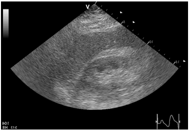
The dataset used in our study consists of 55 B-mode images with dimensions of 434 × 636 pixels, obtained from severely obese patients admitted for bariatric surgery at the Department of General, Transplant, and Liver Surgery, Medical University of Warsaw, Poland. The patients in the dataset are 55 severely obese individuals with a mean age of 40.1±9.1 and a mean BMI of 45.9±5.6. 20% of the patients are male. The ultrasound data was acquired using a GE Vivid E9 Ultrasound System with a sector probe operating at 2.5 MHz. The liver is considered fatty if the hepatic steatosis exceeds 5%. The dataset is publicly available and can be accessed via the Zenodo repository. However, the dataset does not provide specific information about the number of malignant and benign images or the clinical characteristics of the patients [23]. Figure 1 illustrates an example of the images included in the dataset.
Figure 1. A normal image liver image in (A) and an abnormal liver image in (B)
2.2 Images groups
The initial set (group A) was used to create two more sets of images of various sizes that may be used to both train and test the classification models. A qualified sonographer was employed to identify regions of interest (ROIs) in each image. The sonographer's role is to create images of the body's internal structures. This data can then be used to train and develop CNN algorithms for medical diagnosis, disease detection, and other applications. Therefore, sonographers must know anatomy, physiology, US physics, and instrumentation. Each ROI was then cropped in two steps, each with a different size. Fifty-five 180 × 180-pixel images (group B) and hundred and sixty-five 32 × 32-pixel images (group C) were cropped using ImageJ, an image processing application created at the National Institutes of Health and the Laboratory for Optical and Computational Instrumentation (LOCI, University of Wisconsin) [24]. The sizes of the images were selected because they were frequently used in similar studies that discussed AI in US for diagnosing NAFLD [22]. Figure 2 shows images from Group B and Group C.
Figure 2. 128 × 128 and 32 × 32 size images
2.3 Image pre-processing
Variations of an image can be generated using several transformations. Seven image pre-processing approaches were individually used on each image group (A, B, and C) to augment the images. We chose these approaches since they are the most utilized ones in similar studies [22]. Following the application of the process, the number of images in groups A and B increased to 440 and to 1,320 in group C. The seven methods utilized to pre-process the three image sizes are briefly described below.
2.3.1 Resizing
Resizing images is a crucial pre-processing step in computer vision. Downscaled images can improve efficiency and accuracy, as they contain less detail and enable faster training. Resizing also facilitates analysis and interpretation by standardizing image sizes for easier comparison. While full resolution images can increase computation time and reduce performance, downscaled images can be beneficial, particularly for large datasets or limited computing power. Overall, resizing images can enhance the effectiveness of machine learning models. [25]. We discuss the effect of resizing on the performance metrics of the deep learning models later in this study.
2.3.2 Flipping
Flipping is a common data augmentation technique used in computer vision tasks. Flipping an image involves reversing it along a horizontal or vertical axis. A horizontal flip is on the vertical axis, and a vertical flip is on the horizontal axis. Horizontal flip augmentation, utilized in this work, involves reversing all the rows and columns of image pixels horizontally. Horizontal flipping contributes to the model's ability to learn invariant features. Flipping can also help increase the model's robustness to noise and artifacts present in the images [26]. Figure 3 shows an image that has been flipped.
Figure 3. Flipped normal image
2.3.3 Rotating
Random rotation augmentation randomly rotates an entire image's pixels from 0 to 360 degrees. Minor image rotations can significantly alter a classifier’s performance, positively or adversely, without requiring extra data collection. Furthermore, introducing purposeful defects helps the model understand what an item typically looks like. The inclusion of random rotations in the training process allows the model to become more robust to variations in the orientation and alignment of fatty liver ultrasound images [27]. Figure 4 shows an image that has been rotated.
Figure 4. Rotated normal image
2.3.4 Zooming
Zoom augmentation is used to randomly zoom into an image at various levels and may add additional pixels to the image. Random zooming is a type of regularization approach used for training datasets. Random zooming increases training variability and reduces model overfitting [28]. Figure 5 shows an image created after randomly zooming in on part of an image.
Figure 5. Zoomed diseased image
2.3.5 Contrast enhancement
The distinction between light and dark pixels determines an image's contrast. While high-contrast images include vivid highlights and strong shadows, low-contrast images have a limited range of luminance. Contrast augmentation may create new images from old ones while preserving relative shapes and sizes of items in the images, which are commonly lost when using most traditional image augmentation techniques. The accuracy of deep learning models is increased by contrast enhancement, which highlights intensity variations in tissues and reveals patterns for differentiating between normal and fatty liver tissues [29]. Figure 6 shows an image after processing the contrast.
Figure 6. Contrasted diseased image
2.3.6 Brightening
The goal of brightness augmentation is to allow a model trained on diverse illumination conditions to generalize across images. Brightness boosts the image's overall brightness, whereas contrast modifies the contrast between the darkest and brightest colors. Brightening augmentation standardizes lighting conditions in a dataset, enhancing the model's exposure to real-life brightness variations and highlighting subtle grayscale differences, potentially aiding in fatty liver classification patterns [30]. Figure 7 shows an image with brightness modification.
Figure 7. Brightened normal image
Figure 8. Wrapped normal image
2.3.7 Wrapping
Image wrapping is used to increase the accuracy of image recognition models by adding geometric distortions to an image. An existing image is wrapped around a 3D object, like a cube or sphere, to produce a new image. The new image may then be fed to a model as input, enabling the model to gain knowledge from a broader range of data to boost its accuracy. The demand for massive datasets can be alleviated by using image-wrapping augmentation to provide synthetic data for training models [31]. Figure 8 is an example of a wrapped image.
2.4 Classifiers
Deep learning (DL) classifiers are a particular ML algorithm that categorizes data using many ANN layers. Deep learning classifiers are utilized for applications that need supervised learning, including object detection, image classification, and natural language processing. Deep learning classifiers can learn complicated patterns from enormous volumes of data and make predictions about unknown data [32]. Convolutional neural networks (CNNs) are DL neural networks that interpret visual information. Convolutional neural networks' primary applications are image recognition and classification. Convolutional neural networks analyze images and extract features by combining convolutional, pooling, and fully connected layers [33]. In this study, we applied seven different types of CNN classifiers to the three image sets. In the following, we describe the classifiers and provide a motivation for their inclusion in this study.
2.4.1 ResNet50
Microsoft Research created ResNet50, a deep CNN architecture presented in the 2015 ImageNet competition by Kaiming et al. [34]. ResNet50 is a 50-layer deep residual network containing 50 layers of neurons and residual links that not only allow the network to recycle features learned earlier in the network. It is a deep convolutional neural network that can effectively capture complex image features and hierarchical representations. The residual connections in ResNet50 address the “vanishing gradient” problem, making it easier to train deeper networks. ResNet50 has been trained on over one million images from the ImageNet dataset, enabling it to leverage pre-trained weights and transfer learning for various computer vision tasks. However, its computational complexity due to its depth and the large number of parameters can make training and inference slower, and it requires a considerable amount of memory, limiting its suitability for resource-constrained environments.
Nevertheless, ResNet50's high representational capacity and ability to leverage pre-trained weights make it a strong candidate for hepatic steatosis classification, where subtle visual cues may play a crucial role in accurate diagnosis. Its deep architecture can effectively capture intricate features in ultrasound images and extract discriminative features related to hepatic steatosis [35].
2.4.2 ResNet34
ResNet34 is a 34-layer neural network that has been trained on the ImageNet dataset, employing deep residual learning for various applications such as semantic segmentation, object detection, and image classification [34]. It strikes a balance between model complexity and computational efficiency, retaining the advantages of residual connections for effective gradient flow and facilitating the training of deeper models. Although it is less computationally demanding than ResNet50, ResNet34 still has a significant number of parameters, which may limit its deployment in resource-constrained environments. Additionally, its reduced depth compared to ResNet50 might lead to slightly lower performance on complex image classification tasks. However, ResNet34 remains a suitable choice for hepatic steatosis classification as it can capture meaningful features and leverage pre-trained weights, contributing to accurate ultrasound image classification.
2.4.3 ResNet18
ResNet18 is a lightweight variant of the ResNet architecture, making it computationally efficient and memory-friendly. It benefits from residual connections, enabling effective gradient propagation and training of deeper models. Like ResNet50 and ResNet34, ResNet18 has been trained on the ImageNet dataset, allowing for transfer learning [34]. However, the reduced depth of ResNet18 may limit its ability to capture highly intricate features compared to deeper architectures like ResNet50 and ResNet34. It may not perform as well as deeper models on complex image classification tasks. Nevertheless, ResNet18's lightweight nature and computational efficiency make it a potential candidate for hepatic steatosis classification, especially in resource-constrained environments. It can still capture essential image features related to hepatic steatosis and provide reliable results.
2.4.4 AlexNet
AlexNet, proposed by Krizhevsky et al. [36] is another CNN that gained significant attention in the field of computer vision. It won the ImageNet Large Scale Visual Recognition Challenge (ILSVRC) 2012. AlexNet has a relatively simple architecture compared to more recent models, making it computationally efficient and faster to train. It comprises five convolutional layers, three fully linked layers, and one final output layer. AlexNet has demonstrated good performance in various image classification tasks, including the ImageNet challenge. However, compared to more modern architectures, AlexNet may have limitations in capturing highly complex and intricate image features. It may also be prone to overfitting when applied to smaller datasets due to its large number of parameters. While AlexNet can be suitable for the hepatic steatosis classification task, considering its early success in image classification, it may be worth exploring newer models to potentially achieve higher accuracy, given the availability of more advanced architectures.
2.4.5 MobileNet_v2
MobileNet_v2 is a lightweight CNN geared toward mobile and embedded vision applications. It is an upgraded version of the original MobileNet architecture, designed to minimize computational complexity while preserving accuracy. MobileNet_v2 achieves this by reducing parameters and calculations in depth-wise separable convolutions, resulting in a more efficient model [37]. Its advantages include being specifically designed for mobile and resource-constrained devices, striking a good balance between model size and accuracy, and utilizing depth-wise separable convolutions to reduce parameters and computational requirements. It achieves relatively high accuracy while optimized for deployment on devices with limited computational power. However, compared to larger models, MobileNet_v2 may have limitations in capturing fine-grained details and intricate image features, and it may not perform as well as larger models on tasks requiring high precision or dealing with complex image variations. Nevertheless, MobileNet_v2 is suitable for the hepatic steatosis classification task, given the preference for low-cost and resource-efficient methods in ultrasound-based screening. Its optimized design and efficient inference make real-time analysis and deployment on mobile or edge devices practical.
2.4.6 DenseNet121
Huang et al. [38] created the CNN architecture known as DenseNet121 in 2017. A DL architecture of this kind uses numerous connections between layers to enhance information flow and minimize the number of parameters. Each layer in the 121-layer DenseNet121 design is linked to every other layer in a feed-forward method. This architecture has produced cutting-edge results for image classification applications on several datasets. DenseNet121 is a densely connected convolutional neural network that encourages feature reuse and facilitates gradient flow throughout the network. Its dense connectivity patterns allow for better information propagation and feature extraction, leading to improved accuracy. DenseNet121 has demonstrated strong performance on various image classification tasks and is widely used in the computer vision community. However, DenseNet121 has a relatively larger number of parameters compared to some other models, making it computationally more expensive. Training a DenseNet121 model from scratch may require a larger amount of data and computational resources. Nevertheless, DenseNet121 can be well-suited for the hepatic steatosis classification task, given its ability to capture intricate image features and achieve high accuracy. If a considerable amount of labeled training data is available, DenseNet121 can provide robust performance in identifying hepatic steatosis from ultrasound images.
2.4.7 EfficientNet-B0
Google A.I. developed the EfficientNet family of CNN architectures through network architecture search, aiming to optimize the trade-off between input resolution, network depth, and width. EfficientNet-B0, part of this family, enhances accuracy and efficiency while minimizing computational costs. It utilizes depth-wise separable convolutions, squeeze-and-excitation blocks, and compound scaling to capture diverse image features effectively. EfficientNet-B0 has demonstrated state-of-the-art performance in image classification benchmarks, maintaining a compact model size. However, compared to smaller models, it may have slightly higher computational requirements, and training from scratch may necessitate a larger labeled dataset. Nonetheless, it proved successful in the classification task, outperforming other models in terms of accuracy and evaluation metrics. Its balance of accuracy and efficiency makes it a strong candidate for automated analysis of ultrasound images for hepatic steatosis screening [39].
2.5 Stratified k-fold cross-validation
K-fold cross-validation can be used to combat the detrimental effects of small input data sets. By dividing the data into k folds and stratifying (or balancing) each fold according to the target variable, an ML model can be evaluated using the stratified k-fold cross-validation approach. This approach allows the model to use more significant amounts of data (k-1 folds) while still offering statistically significant validation on the left-out fold. As a result, k-fold cross-validation minimizes bias and variance in the model assessment process by ensuring that each fold is representative of the whole dataset [40]. Generalized Cross-Validation (GCV) is a useful technique for testing different combinations of parameter values and selecting the best results, especially when analyzing data with outliers and multicollinearity problems. Roozbeh et al. found that using GCV allowed them to simultaneously optimize multiple parameters in the prediction model, making the model more accurate and effective. Therefore, GCV can be a useful tool for improving the performance of a prediction model [41]. However, GCV and cross-validation (CV) are more general types of validation methods that do not consider the class distribution of the dataset. They may not be as effective for prediction purposes when dealing with imbalanced datasets, as they can lead to biased models that are overly focused on the majority class. In contrast, stratified cross-validation is particularly useful for prediction tasks when dealing with imbalanced datasets. K-fold cross-validation has several advantages over other model evaluation techniques, such as allowing the use of all the data for training and testing, reducing variance, and being more computationally efficient. To compare the performance of the proposed criteria with other criteria, we use metrics such as accuracy, precision, recall, and F1-score. Our results show that the proposed criteria outperformed the traditional k-fold cross-validation in terms of accuracy, precision, recall, and F1-score. This suggests that the proposed criteria are a competitive choice over other criteria for model evaluation and comparison.
2.6 Network training
For this study, we unify the values of different training parameters in all 21 experiments to compare the results among different image sizes and classifiers. The values were evaluated based on preliminary investigations, prior experiences, or published studies. We split the dataset into two parts. We use 20% for validation and 80% for training. In addition, we set the batch size to eight. Ten folds are used for cross-validation, and 20 epochs are used in each fold. The learning rate ranges between $1 \times 10^{-6}$ and $1 \times 10^{-3}$ for all the experiments, using learning rate scheduling. The learning rate and patch number were adjusted based on the model's performance during training. Monitoring performance metrics such as accuracy and loss during training is essential for making informed decisions.
This study utilizes Google Colaboratory ("Colab" for short). This web-based Jupyter interface provides a runtime for DL and free-of-charge access to a Graphics Processing Unit (GPU), such as Tesla K80 or Tesla T4, with 12 to 16 GB of dedicated video memory. Colab’s default virtual machines also provide pre-installed common deep learning and data science modules, specifically including FastAI, a high-level API for transfer learning. FastAI offers a convenient interface for building and training neural networks and accessing pre-trained models for image classification, tools for data augmentation, model selection, and hyperparameter tuning.
2.7 Model evaluation
Deep learning model assessments determine how well a DL model performs on a given dataset. This process entails measuring some metrics to see how effectively the model performs. In this study, we use six metrics to evaluate each model. The metrics' findings are based on picking the best overall fold epoch outcomes and averaging them.
In this study, the metric equations make use of several concepts, including the distinction between a "normal" (-Ve) image and an "abnormal" (+Ve) image, as determined by the biopsy results. There are only four possible outcomes for each image: true positive (TP), true negative (TN), false positive (FP), and false negative (FN). The cases are as follows: TP—the image is "abnormal," and the prediction is +Ve; TN—the image is "normal," and the prediction is -Ve; FP—the image is "normal," and the prediction is +Ve; and FN—the image is "abnormal," and the prediction is -Ve.
2.7.1 Accuracy
Accuracy measures how accurately a model can predict the correct outcome. It is calculated by dividing the number of correct predictions by the total number of predictions:
Accuracy $=(T P+T N) /(T P+F P+F N+T N)$
2.7.2 Sensitivity
Sensitivity measures how well a model can identify positive outcomes. It is calculated by dividing the number of true positives (TP; correctly identified positive outcomes) by the total number of actual positives (all positive outcomes):
Sensitivity $=T P /(T P+F N)$
2.7.3 Specificity
Specificity measures how well a model can identify negative outcomes. It is calculated by dividing the number of true negatives (TN; correctly identified negative outcomes) by the total number of actual negatives (all negative outcomes):
Specificity $=T N /(T N+F P)$
2.7.4 Precision
Precision measures how precise a model's predictions are. It is calculated by dividing the number of true positives (TP; correctly identified positive outcomes) by the total number of predicted positives (all predicted positive outcomes):
Precision $=T P /(T P+F P)$
2.7.5 F1 score
The F1 score is a measure that combines both Precision and Sensitivity into one metric. It is calculated as the harmonic mean of precision and recall, and ranges from 0 to 1, with 1 being perfect accuracy:
$\begin{gathered}\text { F1 Score }=2 *(\text { Recall } * \text { Precision }) /(\text { Recall }+ \text { Precision })\end{gathered}$
2.7.6 Matthews Correlation Coefficient (MCC)
MCC is a measure that combines accuracy, sensitivity, specificity, precision, and F1 score into one metric. It ranges from -1 to 1, with higher values indicating better performance:
$M C C=\frac{T P \times T N-F P \times F N}{\sqrt[2]{(T P+F P)(T P+F N)(T N+F P)(T N+F N)}}$
In this work, we developed a working technique, wherein three sets of various-sized images were created to determine which is better at diagnosing disease. Seven additional processing techniques were used on the images to increase quantity and training variety, lessen overfitting, and achieve other objectives. We also considered seven DL classifiers with encouraging classifying image results reported in scientific publications. A stratified k-fold cross-validation strategy was utilized, with 20 folds and 20 epochs, to prevent issues such as overfitting and data leaking and to make the best use of the data. Six metrics of the best epoch in each fold were averaged.
Table 1. Results for Group A
|
Model |
Average Accuracy |
Average Sensitivity |
Average Specificity |
Average Precision |
Average F1 Score |
Mean of MCC |
|
EfficientNet-B0 |
0.989 |
0.986 |
0.990 |
0.979 |
0.982 |
0.974 |
|
ResNet34 |
0.967 |
0.936 |
0.982 |
0.963 |
0.946 |
0.926 |
|
AlexNet |
0.948 |
0.868 |
0.985 |
0.966 |
0.909 |
0.880 |
|
Densnet121 |
0.945 |
0.936 |
0.949 |
0.897 |
0.914 |
0.876 |
|
ResNet18 |
0.939 |
0.861 |
0.975 |
0.944 |
0.896 |
0.859 |
|
ResNet50 |
0.910 |
0.868 |
0.930 |
0.860 |
0.860 |
0.860 |
|
MobileNet_v2 |
0.806 |
0.732 |
0.839 |
0.682 |
0.700 |
0.564 |
Table 2. Results for Group B
|
Model |
Average Accuracy |
Average Sensitivity |
Average Specificity |
Average Precision |
Average F1 Score |
Mean of MCC |
|
EfficientNet-B0 |
0.984 |
0.996 |
0.979 |
0.956 |
0.976 |
0.965 |
|
ResNet34 |
0.926 |
0.918 |
0.930 |
0.864 |
0.888 |
0.836 |
|
ResNet18 |
0.919 |
0.907 |
0.925 |
0.848 |
0.874 |
0.818 |
|
DensNet121 |
0.904 |
0.882 |
0.915 |
0.828 |
0.853 |
0.785 |
|
AlexNet |
0.846 |
0.704 |
0.911 |
0.785 |
0.738 |
0.635 |
|
ResNet50 |
0.844 |
0.771 |
0.877 |
0.756 |
0.755 |
0.650 |
|
MobileNet_v2 |
0.764 |
0.454 |
0.907 |
0.695 |
0.532 |
0.413 |
Table 3. Results for Group C
|
Model |
Average Accuracy |
Average Sensitivity |
Average Specificity |
Average Precision |
Average F1 Score |
Mean of MCC |
|
EfficientNet-B0 |
0.9634 |
0.9220 |
0.9820 |
0.9548 |
0.9317 |
0.9126 |
|
Densnet121 |
0.7223 |
0.1390 |
0.9836 |
0.7619 |
0.2265 |
0.2347 |
|
MobileNet_v2 |
0.7200 |
0.1988 |
0.9536 |
0.6830 |
0.2983 |
0.2447 |
|
ResNet18 |
0.7147 |
0.2159 |
0.9383 |
0.6434 |
0.2963 |
0.2217 |
|
ResNet34 |
0.7000 |
0.0951 |
0.9710 |
nan |
0.1510 |
0.1448 |
|
ResNet50 |
0.6992 |
0.1622 |
0.9399 |
0.5374 |
0.2400 |
0.1575 |
|
AlexNet |
0.6958 |
0.0756 |
0.9738 |
nan |
0.1294 |
0.1178 |
Table 4. Results of the EfficientNet-B0 classifier
|
Image Size |
Average Accuracy |
Average Sensitivity |
Average Specificity |
Average Precision |
Average F1 Score |
Mean of MCC |
|
Group A |
0.989 |
0.986 |
0.990 |
0.979 |
0.982 |
0.974 |
|
Group B |
0.984 |
0.996 |
0.979 |
0.956 |
0.976 |
0.965 |
|
Group C |
0.963 |
0.922 |
0.982 |
0.955 |
0.932 |
0.913 |
Table 5. Results of the ResNet34
|
Image Size |
Average Accuracy |
Average Sensitivity |
Average Specificity |
Average Precision |
Average F1 Score |
Mean of MCC |
|
Group A |
0.967 |
0.936 |
0.982 |
0.963 |
0.946 |
0.926 |
|
Group B |
0.926 |
0.918 |
0.930 |
0.864 |
0.888 |
0.836 |
|
Group C |
0.700 |
0.095 |
0.971 |
NaN |
0.151 |
0.145 |
Table 6. Results of the AlexNet classifier
|
Image Size |
Average Accuracy |
Average Sensitivity |
Average Specificity |
Average Precision |
Average F1 Score |
Mean of MCC |
|
Group A. |
0.948 |
0.868 |
0.985 |
0.966 |
0.909 |
0.880 |
|
Group B |
0.846 |
0.704 |
0.911 |
0.785 |
0.738 |
0.635 |
|
Group C |
0.696 |
0.076 |
0.974 |
NaN |
0.129 |
0.118 |
Table 7. Results of the Densnet121 classifier
|
Image Size |
Average Accuracy |
Average Sensitivity |
Average Specificity |
Average Precision |
Average F1 Score |
Mean of MCC |
|
Group A |
0.945 |
0.936 |
0.949 |
0.897 |
0.914 |
0.876 |
|
Group B |
0.904 |
0.882 |
0.915 |
0.828 |
0.853 |
0.785 |
|
Group C |
0.722 |
0.139 |
0.984 |
0.762 |
0.226 |
0.235 |
Table 8. Results of the Mobilnet_v2 classifier
|
Image Size |
Average Accuracy |
Average Sensitivity |
Average Specificity |
Average Precision |
Average F1 Score |
Mean of MCC |
|
Group A |
0.806 |
0.732 |
0.839 |
0.682 |
0.700 |
0.564 |
|
Group B |
0.764 |
0.454 |
0.907 |
0.695 |
0.532 |
0.413 |
|
Group C |
0.720 |
0.199 |
0.954 |
0.683 |
0.298 |
0.245 |
Table 9. Results of the ResNet18
|
Image Size |
Average Accuracy |
Average Sensitivity |
Average Specificity |
Average Precision |
Average F1 Score |
Mean of MCC |
|
Group A |
0.939 |
0.861 |
0.975 |
0.944 |
0.896 |
0.859 |
|
Group B |
0.919 |
0.907 |
0.925 |
0.848 |
0.874 |
0.818 |
|
Group C |
0.715 |
0.216 |
0.938 |
0.643 |
0.296 |
0.222 |
Table 10. Results of the ResNet50
|
Image Size |
Average Accuracy |
Average Sensitivity |
Average Specificity |
Average Precision |
Average F1 Score |
Mean of MCC |
|
Group A |
0.910 |
0.868 |
0.930 |
0.860 |
0.860 |
0.860 |
|
Group B |
0.844 |
0.771 |
0.877 |
0.756 |
0.755 |
0.650 |
|
Group C |
0.699 |
0.162 |
0.940 |
0.537 |
0.240 |
0.158 |
Table 1 shows the results of the seven classifiers on the full images. The accuracy, sensitivity, specificity, precision, F1 score, and MCC of the EfficientNet-B0, ResNet34, Densnet121, and AlexNet models are all very high. These results indicate that the models perform well and can accurately classify digital ultrasound images. In addition, our data augmentation approach allows us to train generalizing models with smaller datasets, which if of high importance for many medical applications. These models outperformed traditional image analysis and classification techniques, such as manual interpretation by medical professionals or rule-based algorithms. The implications of these findings are significant, as they suggest that DL classifiers can provide accurate and efficient diagnoses for various diseases using digital ultrasound images. This could improve patient outcomes by enabling earlier detection and treatment of diseases. However, considering other factors, such as the model's interpretability, robustness, and computational efficiency, is crucial when selecting a model for a classification task.
Table 2 shows the results of the seven classifiers on the 128 × 128-pixel images. AlexNet and the other classifiers show a varying decrease in performance compared to their results on the full images. However, the accuracy, sensitivity, specificity, precision, F1 score, and MCC are still very high for EfficientNet-B0, ResNet34, and ResNet18, which indicates that the models still perform well and can accurately classify digital ultrasound images. This suggests that DL classifiers can potentially be used for disease diagnosis even with lower-resolution images, which can be beneficial when high-resolution images are not available or feasible, especially considering the higher computational requirements to train and predict using large images. However, the robustness of these models can be affected by variations in image quality, such as differences in lighting or image artifacts, which can lead to misclassifications. This can concern medical professionals who need to understand the reasoning behind a diagnosis to make informed treatment decisions. it is important to note that these results are specific to the dataset and classification task used in the study. The performance of these models may vary depending on the type of disease or imaging modality being analyzed, and further research is needed to understand the potential of DL classifiers in disease diagnosis fully.
Table 3 shows the results of the seven classifiers on the 32 × 32-pixel images. The accuracy, sensitivity, specificity, precision, F1 score, and MCC are very high for EfficientNet-B0, indicating that the model still performs well and can accurately classify binary ultrasound images. However, all the other classifiers show a varying decrease in performance compared to their results on the other two groups of images. Since most of the results are unacceptable, there is a need to focus more on the details when image sizes are small. However, it is important to consider the trade-off between image resolution and computational efficiency when selecting a model for a classification task. Additionally, these models' interpretability, robustness, and computational efficiency should also be considered when selecting a model for a classification task.
Table 4 shows the results of the EfficientNet-B0 classifier on the three groups of images. The accuracy of the EfficientNet-B0 model was 0.989 for group A, meaning it correctly identified 98.9% of the images it was tested on. The same can be said for groups B and C, whose results were 0.984 and 0.963, respectively. The average sensitivity of the Efficient-Net-B0 model on group A image was 0.986, which means that it correctly identified 98.6% of the positive cases (i.e., those with a disease). Also the same can be said for groups B and C, whose results were 0.996 and 0.922, respectively. The specificity of the EfficientNet-B0 model on group A images was 0.990, which means that it correctly identified 99% of the negative cases (i.e., those without a disease). The same can be said for groups B and C, whose results were 0.979 and 0.982, respectively. The precision of the EfficientNet-B0 model on group A images was 0.979, which means that out of all the cases it predicted as positive, 97.9% were positive. Again, the same can be said for groups B and C, whose results were 0.956 and 0.955, respectively. The F1 score measures the model's accuracy and precision and indicates how well it can distinguish between positive and negative cases. The EfficientNet-B0 model's F1 score for group A, B, and C images were 0.982, 0.976, and 0.932, respectively. Finally, Matthew’s Correlation Coefficient (MCC) for the Efficient-Net-B0 model on group A images measures the model's ability to classify both positive and negative cases correctly and indicates how well it can distinguish between them, which was 0.974. Groups B and C had similar results, with 0.965 and 0.913, respectively. As demonstrated later in this study, EfficientNet-B0 delivers better inference on all image groups than the other classifiers but is slower in training, which may influence subsequent deployment.
Table 5 shows the results of the ResNet34 classifier on the three groups of images. The average accuracy, sensitivity, and specificity of groups A and B scored high. On the other hand, the values for average precision and average F1 Score for group B decrease compared to group A, which indicates a reduction in the classifier's ability to distinguish different classes in smaller image sizes. By contrast, all the metrics scored very low for group C images. This fact is evidence that the ResNet34 classifier cannot binarily classify very small-size ultrasound images with the described model parameters. This verity is more evident due to the NaN value achieved for precision. NaN is not a valid value for accuracy and indicates an error in the data or an issue with the classifier.
Although Densnet121, ResNet18, ResNet50, and AlexNet all had similar results for the group A and group B images, they were less efficient than EfficientNet-B0 and Res-Net34. Except for EfficientNet-B0 and ResNet34, all classifiers performed poorly on group C images. Tables 6, 7, 8, 9, and 10 include the metrics' results for the three image groups for AlexNet, Densnet121, MobileNet_v2, Densnet18, and ResNet50, respectively.
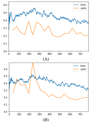
A learning curve is a graphical representation of a model's performance over time. The curves in Figures 9–11 were created by graphing the model's training and validation performance measures, such as accuracy and loss, against the number of training epochs. These metrics were collected during the k-fold cross-validation process, which separated the dataset into k subsets. To produce the learning curves, the average training and validation performance metrics over the k folds were computed and shown for each epoch. These curves give useful information about the model's performance as well as potential overfitting or underfitting concerns during training. Curve may be used to identify regions of a model that are underperforming and to decide whether model adjustments are required. A learning curve may also be used to compare various models, determine which performs best, and determine how effectively a model generalizes to previously unknown data [42]. In this study, the learning curves show that most classifiers cannot easily learn from the training dataset of group C images. Figure 9A shows AlexNet was an underfit model for analyzing group C images. The flat line indicates that the model could not learn the training dataset easily. After increasing the number of epochs, the model failed to transition from underfitting to overfitting, which indicates that this model should be rejected for this application. Notice that with group C images AlexNet results in a NaN result, showing the weakness of the classifier with this set of images. The same behavior can be seen with most classifiers. Figure 9B illustrates that even EfficientNet-B0 exhibits a similar pattern, indicating that extremely tiny images may require additional arrangements, such as adding regularization or tuning the hyperparameter, to remove underfitting.
In contrast, EfficientNet-B0 fits well with the full images in Figure 10A. In addition, Densnet121 shows good fitting in Figure 10B despite the noise and fluctuations, which indicate less stability compared to EfficientNet-B0.
When analyzing learning curves, an unrepresentative validation dataset is a concern. Validation loss with noisy movements around the training loss or lower than the training loss suggests that the validation dataset does not give enough information to evaluate the model's generalization ability. Figure 11 shows examples of curves that indicate an unrepre-sentative validation dataset.
Figure 9. Learning Curve for: (A) the ninth fold of AlexNet and (B) the seventh fold of Efficient-Net-B0 on 32x32 sized images
Figure 10. Learning Curve for: (A) the fourth fold of EfficientNet-B0 and (B) the eighth fold of Densnet121 on full-sized images
Figure 11. Learning Curve for: (A) the fifth fold of ResNet34 and (B) the eighth fold of ResNet18 on 128 × 128 pixel images
Overall, the learning curves in Figures 9-11 provide useful insights into the performance of different classifiers on different-sized images. The patterns observed in these curves can be used to identify regions of the model that are underperforming and to determine whether model adjustments are required. Additionally, these curves can be used to compare different models' performance and determine which model performs best on a given classification task.
The studies in Table 11 all use the same images as a dataset but employ different A.I. classifiers, which have varying levels of complexity, and achieve varying levels of accuracy. EfficientNet-B0 achieved an accuracy of 98.90%, the highest among all the studies used for the dataset, suggesting that this algorithm is highly effective for image classification tasks. Overall, the more complex A.I. classifiers achieve higher accuracies than simpler ones. It is also worth noting that even though some A.I. classifiers have higher accuracies than others, they may not be suitable for specific tasks due to their computational complexity, cost, required training time, or other factors. Therefore, it is essential to consider all aspects when selecting which A.I. classifier to use for a given task or dataset. The fact that the studies in the table achieved high levels of accuracy with a small dataset is impressive and suggests that A.I. classifiers can be a valuable tool for medical image analysis. However, it is important to note that the results of these studies should be validated on larger datasets and in clinical settings before being used in practice.
Table 11. Accuracy summary for different models
|
Reference Number |
Author |
A.I. Classifier |
Accuracy |
|
[23] |
Byra et al. |
support vector machine (SVM) |
96.3% |
|
[43] |
Zamanian et al. |
SVM |
98.64% |
|
[44] |
Mohammad & Almekkawy |
Fourier Convolutional Neural Networks (FCNN) ((6 layers)) |
84.40% |
|
[45] |
Mohammad & Almekkawy |
Inception-ResNet-v2 |
98.50% |
|
[46] |
Simion et al. |
CNN (4 convolutional layers) |
87.49% |
|
[47] |
Che |
multi-scale two-dimensional mid-fusion residual neural network (ResNet) |
91.31% |
|
|
Proposed Method |
EfficientNet-B0 |
98.90% |
Table 12. Comparison with Support Vector Machine classifier results on the same dataset
|
Reference Number |
Author |
Cross-Validation |
Feature Extraction Method |
Classifier |
Accuracy |
Sensitivity |
Specificity |
|
[23] |
Byra et al. |
5-fold Leave-one-out |
Inception-ResNet-v2 |
SVM |
96.3% |
100% |
88.2% |
|
[43] |
Zamanian et al. |
10-fold |
Inception-ResNetV2, GoogleNet, AlexNet, ResNet101 |
SVM |
98.64% |
97.20% |
100% |
|
|
Proposed Method |
Stratified 10-fold |
EfficientNet-B0 |
EfficientNet-B0 |
98.90% |
98.6% |
99.0% |
Table 13. Summary of our experiments. All results in %. A: Full images; B: 128 × 128 images; C: 32 × 32 images
|
EfficientNet-B0 |
ResNet34 |
AlexNet |
DensNet121 |
ResNet18 |
ResNet50 |
MobileNet_v2 |
|||||||||||||||
|
|
A |
B |
C |
A |
B |
C |
A |
B |
C |
A |
B |
C |
A |
B |
C |
A |
B |
C |
A |
B |
C |
|
Accuracy |
98.9 |
98.4 |
96.3 |
96.7 |
92.6 |
70.0 |
94.8 |
84.6 |
69.6 |
94.5 |
90.4 |
72.2 |
93.9 |
91.9 |
71.5 |
91.0 |
84.4 |
69.9 |
80.6 |
76.4 |
72.0 |
|
Sensitivity |
98.6 |
99.6 |
92.2 |
93.6 |
91.8 |
9.5 |
86.8 |
70.4 |
7.6 |
93.6 |
88.2 |
13.9 |
86.1 |
90.7 |
21.6 |
86.8 |
77.1 |
16.2 |
73.2 |
45.4 |
19.9 |
|
Specifi-city |
99.0 |
97.9 |
98.2 |
98.2 |
93.0 |
97.1 |
98.5 |
91.1 |
97.4 |
94.9 |
91.5 |
98.4 |
97.5 |
92.5 |
93.8 |
93.0 |
87.7 |
94.0 |
83.9 |
90.7 |
95.4 |
|
Precision |
97.9 |
95.6 |
95.5 |
96.3 |
86.4 |
nan |
96.6 |
78.5 |
nan |
89.7 |
82.8 |
76.2 |
94.4 |
84.8 |
64.3 |
86.0 |
75.6 |
53.7 |
68.2 |
69.5 |
68.3 |
|
F1 |
98.2 |
97.6 |
93.2 |
94.6 |
88.8 |
15.1 |
90.9 |
73.8 |
12.9 |
9.14 |
85.3 |
22.6 |
89.6 |
87.4 |
29.6 |
86.0 |
75.5 |
24.0 |
70.0 |
53.2 |
29.8 |
|
Mean of mcc |
97.4 |
96.5 |
91.3 |
92.6 |
83.6 |
14.5 |
88.0 |
63.5 |
11.8 |
87.6 |
78.5 |
23.5 |
85.9 |
81.8 |
22.2 |
86.0 |
65.0 |
15.8 |
56.4 |
41.3 |
24.5 |
Finally, and in the context of fatty liver classification, the authors chose Support Vector Machines (SVM) as a comparison point to demonstrate the superiority of deep learning techniques, specifically the EfficientNet-B0 model. However, it is important to note that SVM has its own advantages, such as computational efficiency and a strong theoretical foundation. The SVM is a popular machine learning algorithm used for classification and regression analysis. It works by finding the best hyperplane that separates the data into different classes, maximizing the margin between the two classes. SVM has been widely used in various fields, including image classification, text classification, and bioinformatics. While the comparison with SVM provides a useful benchmark, it is not the only possible comparison point. Other machine learning algorithms, such as decision trees, random forests, and neural networks, could also be used for comparison. The choice of comparison point may depend on the specific characteristics of the dataset and the task at hand. When comparing the EfficientNet-B0 model with an SVM classifier in terms of accuracy, sensitivity, and specificity, the authors found that the EfficientNet-B0 model surpassed the SVM classifier, as indicated in Table 12. However, it is important to consider that the outcome may be influenced if the studies being compared used different datasets, pre-processing methodologies, model architectures, and hyper-parameters. We also share at the end all the results from all the experiments in Table 13 for a comprehensive look at the work.
There are various limitations to this study that should be noted. To begin, the results may be limited in their generalizability because the image dataset was created using open-source data, which may not be representative of the larger population. Additionally, because the study concentrated on the binary diagnosis of hepatic steatosis using ultrasound images, the findings may not be applicable to other types of liver disorders or imaging modalities. Second, potential bias may have been introduced during image collection and selection, as the study did not provide information on this process. To mitigate this issue, the study employed seven distinct image pre-processing methods to augment the dataset. This approach aimed to reduce the impact of any biases or artifacts introduced during the image collection and selection process. Additionally, the study utilized various metrics to evaluate the performance of the models, which further aided in mitigating the impact of any biases or artifacts in the dataset. Finally, by comparing the loss curves of different models, researchers could identify the most effective model with the lowest loss value. This comparison helped ensure that the model accurately detected hepatic steatosis in ultrasound images without being influenced by any biases or artifacts in the dataset. Third, while the study employed seven distinct image pre-processing methods to augment the dataset, some of these methods may have introduced bias or artifacts into the images, which may have influenced the results. Each image pre-processing technique should be examined independently to see how much of a positive or negative influence it has on classification results. Fourth, the choice of metrics may have impacted the evaluation of the models' performance, as various metrics may provide different findings. More training data is also required to generalize the model's output and lessen the risk of underfitting. Furthermore, while EfficientNet-B0 was discovered to be the best accurate mod-el, its computing efficiency should be taken into account for practical applications. Lastly, future research should look at different classifiers and EfficientNet family members to find the best model in terms of accuracy and computing efficiency.
Several methods were used to pre-process the NAFLD US images before utilizing stratified cross-validation with various CNN classifiers. As a result, EfficientNet-B0 had the highest average accuracy, specificity, and sensitivity of all the classifiers. This might be related to the Network Architecture Search behind the EfficientNet family that searches for the best performing architecture given a computational budget. EfficientNet-B0 combines CNNs and transfer learning to discover image patterns, the Squeeze-Excitation activation, which is a mechanism that recalibrates channel-wise feature responses, and a network's capacity.
More training data is required to generalize models' outputs further. In addition, despite the image augmentation and fold cross-validation processes implemented to ensure maximum benefit of the data set, additional validation data is required to guarantee that models are not underfitting. Finally, this study discovered that tiny images are challenging to classify effectively; hence full and medium-sized images are preferable. Based on the findings of this investigation, it is possible to infer that EfficientNet-B0, ResNet34, and DensNet121 have promising potential for fatty liver U.S. image classification tasks.
In the future, each image pre-processing technique should be examined independently to see how much of a positive or negative influence it has on classification results. Collaborating with other research groups and institutions could prove fruitful for acquiring additional datasets. Furthermore, exploring alternative imaging modalities or integrating other clinical data, such as blood tests or medical histories, could further enhance the accuracy and generalizability of our model in the future. Other classifiers, such as CNN or classic ML, must also be tested to determine the optimum accuracy and computing efficiency model. Newer and more advanced architectures such as ResNet152, and Inception-v4 can be investigated in future. Other members of the EfficientNet family such as EfficientNet-B7 can be examined as well. One potential benefit of using other members of the EfficientNet family is that they are designed to balance model size and accuracy, which could result in better performance on our task. Additionally, these models have good generalization capabilities, meaning they can perform well on a wide range of tasks and datasets. However, one challenge we may face is the increased computational cost of using larger models, which may limit our ability to train and evaluate these models on our current hardware. Another challenge is the potential for overfitting when using very large models, which we will need to address by carefully optimizing our training procedures and possibly incorporating regularization techniques. In addition, when many images are available, an image classification system that can classify stages of the whole disease, rather than the present binary classification, should be used. The shift from binary classification to classifying disease stages has significant implications for model development and real-world applications. Classifying disease stages helps understand progression, identify early warning signs, and improve patient outcomes. However, this presents challenges in data collection and labeling, as multiple stages of the disease need to be collected and labeled. Additionally, adapting models to individual patient profiles is necessary due to disease progression variations among individuals. Finally, when assessing various methods, including CV, G.C.V., and others, it is advisable to compare their performance on a validation set or through other channels. This can be done by evaluating their prediction accuracy, computational efficiency, and interpretability. One approach is to train each method on a training set and then assess their performance on a separate validation set. Another approach is to analyze the results of experiments or simulations, or conduct a literature review to compare the prediction accuracy, computational efficiency, and interpretability of different methods. Ultimately, the most suitable approach will depend on the specific application and the available resources.
[1] Turing, A.M. (2009). Computing Machinery and Intelligence. In: Epstein, R., Roberts, G., Beber, G. (eds) Parsing the Turing Test. Springer, Dordrecht. https://doi.org/10.1007/978-1-4020-6710-5_3
[2] Kaul, V., Enslin, S., Gross, S.A. (2020). History of artificial intelligence in medicine. Gastrointestinal Endoscopy, 92(4): 807-812. https://doi.org/10.1016/j.gie.2020.06.040
[3] Le Berre, C., Sandborn, W.J., Aridhi, S., Devignes, M.D., Fournier, L., Smaïl-Tabbone, M., Danese, S., Peyrin-Biroulet, L. (2020). Application of artificial intelligence to gastroenterology and hepatology. Gastroenterology, 158(1): 76-94. https://doi.org/10.1053/j.gastro.2019.08.058
[4] Yadav, S.S., Jadhav, S.M. (2019). Deep convolutional neural network based medical image classification for disease diagnosis. Journal of Big Data, 6(1): 1-18. https://doi.org/10.1186/s40537-019-0276-2
[5] LeCun, Y., Bengio, Y., Hinton, G. (2015). Deep learning. Nature, 521(7553): 436-444. https://doi.org/10.1038/nature14539
[6] Huang, Q., Zhang, F., Li, X. (2018). Machine learning in ultrasound computer-aided diagnostic systems: A survey. BioMed Research International, 2018: 5137904. https://doi.org/10.1155/2018/5137904
[7] Hosny, A., Parmar, C., Quackenbush, J., Schwartz, L.H., Aerts, H.J. (2018). Artificial intelligence in radiology. Nature Reviews Cancer, 18(8): 500-510. https://doi.org/10.1038/s41568-018-0016-5
[8] Esteva, A., Kuprel, B., Novoa, R.A., Ko, J., Swetter, S.M., Blau, H.M., Thrun, S. (2017). Dermatologist-level classification of skin cancer with deep neural networks. Nature, 542(7639): 115-118. https://doi.org/10.1038/nature21056
[9] Wong, S.T. (2018). Is pathology prepared for the adoption of artificial intelligence? Cancer cytopathology, 126(6): 373-375. https://doi.org/10.1002/cncy.21994
[10] Gulshan, V., Peng, L., Coram, M., Stumpe, M.C., Wu, D., Narayanaswamy, A., Webster, D.R. (2016). Development and validation of a deep learning algorithm for detection of diabetic retinopathy in retinal fundus photographs. JAMA, 316(22): 2402-2410. https://doi.org/10.1001/jama.2016.17216
[11] Beeman, S.C., Garbow, J.R. (2018). Imaging and Metabolism. Springer, New York.
[12] Adams, L.A., Harmsen, S., Sauver, J.L.S., Charatcharoenwitthaya, P., Enders, F.B., Therneau, T., Angulo, P. (2010). Nonalcoholic fatty liver disease increases risk of death among patients with diabetes: A community-based cohort study. The American Journal of Gastroenterology, 105(7): 1567-1573. https://doi.org/10.1038/ajg.2010.18
[13] Adams, L.A., Anstee, Q.M., Tilg, H., Targher, G. (2017). Non-alcoholic fatty liver disease and its relationship with cardiovascular disease and other extrahepatic diseases. Gut, 66(6): 1138-1153. http://doi.org/10.1136/gutjnl-2017-313884
[14] Tapper, E.B., Lok, A.S.F. (2017). Use of liver imaging and biopsy in clinical practice. New England Journal of Medicine, 377(8): 756-768. https://doi.org/10.1056/NEJMra1610570
[15] Lăpădat, A.M., Jianu, I.R., Ungureanu, B.S., Florescu, L.M., Gheonea, D.I., Sovaila, S., Gheonea, I.A. (2017). Non-invasive imaging techniques in assessing non-alcoholic fatty liver disease: A current status of available methods. Journal of Medicine and Life, 10(1): 19-26.
[16] Petroff, D., Blank, V., Newsome, P.N., et al. (2021). Assessment of hepatic steatosis by controlled attenuation parameter using the M and XL probes: An individual patient data meta-analysis. The Lancet Gastroenterology & Hepatology, 6(3): 185-198. https://doi.org/10.1016/S2468-1253(20)30357-5
[17] Sasso, M., Beaugrand, M., De Ledinghen, V., Douvin, C., Marcellin, P., Poupon, R., Sandrin, L., Miette, V. (2010). Controlled attenuation parameter (CAP): A novel VCTE™ guided ultrasonic attenuation measurement for the evaluation of hepatic steatosis: Preliminary study and validation in a cohort of patients with chronic liver disease from various causes. Ultrasound in Medicine & Biology, 36(11): 1825-1835. https://doi.org/10.1016/j.ultrasmedbio.2010.07.005
[18] Thiele, M., Rausch, V., Fluhr, G., et al. (2018). Controlled attenuation parameter and alcoholic hepatic steatosis: Diagnostic accuracy and role of alcohol detoxification. Journal of Hepatology, 68(5): 1025-1032. https://doi.org/10.1016/j.jhep.2017.12.029
[19] Bedogni, G., Bellentani, S., Miglioli, L., Masutti, F., Passalacqua, M., Castiglione, A., Tiribelli, C. (2006). The Fatty Liver Index: A simple and accurate predictor of hepatic steatosis in the general population. BMC Gastroenterology, 6(1): 1-7. https://doi.org/10.1186/1471-230X-6-33
[20] Webb, M., Yeshua, H., Zelber-Sagi, S., Santo, E., Brazowski, E., Halpern, Z., Oren, R. (2009). Diagnostic value of a computerized hepatorenal index for sonographic quantification of liver steatosis. American Journal of Roentgenology, 192(4): 909-914. https://doi.org/10.2214/AJR.07.4016
[21] Ambinder, E.P. (2005). A history of the shift toward full computerization of medicine. Journal of Oncology Practice, 1(2): 54-56. https://doi.org/10.1200/jop.2005.1.2.54
[22] Alshagathrh, F.M., Househ, M.S. (2022). Artificial intelligence for detecting and quantifying fatty liver in ultrasound images: A systematic review. Bioengineering, 9(12): 748. https://doi.org/10.3390/bioengineering9120748
[23] Byra, M., Styczynski, G., Szmigielski, C., Kalinowski, P., Michałowski, Ł., Paluszkiewicz, R., Ziarkiewicz-Wróblewska, B., Zieniewicz, K., Sobieraj, P., Nowicki, A. (2018). Transfer learning with deep convolutional neural network for liver steatosis assessment in ultrasound images. International Journal of Computer Assisted Radiology and Surgery, 13: 1895-1903. https://doi.org/10.1007/s11548-018-1843-2
[24] Schneider, C.A., Rasband, W.S., Eliceiri, K.W. (2012). NIH Image to ImageJ: 25 years of image analysis. Nature Methods, 9(7): 671-675. https://doi.org/10.1038/nmeth.2089
[25] Saponara, S., Elhanashi, A. (2021). Impact of image resizing on deep learning detectors for training time and model performance. In International Conference on Applications in Electronics Pervading Industry, Environment and Society (pp. 10-17). Cham: Springer International Publishing.
[26] Brinkmann, R. (2008). The Art and Science of Digital Compositing: Techniques for Visual Effects, Animation and Motion Graphics. Morgan Kaufmann.
[27] Engstrom, L., Tran, B., Tsipras, D., Schmidt, L., Madry, A. (2018). A rotation and a translation suffice: Fooling CNNs with simple transformations. ICLR 2019 Conference.
[28] Rahat, M., Hasan, M., Hasan, M.M., Islam, M.T., Rahman, M.S., Islam, A.K., Rahman, M.M. (2021). Deep CNN-based mango insect classification. In: Uddin, M.S., Bansal, J.C. (eds) Computer Vision and Machine Learning in Agriculture. Algorithms for Intelligent Systems. Springer, Singapore. https://doi.org/10.1007/978-981-33-6424-0_5
[29] Merchant, A., Syed, T., Khan, B., Munir, R. (2018). Appearance-based data augmentation for image datasets using contrast preserving sampling. In 2018 24th International Conference on Pattern Recognition (ICPR), Beijing, China, pp. 1235-1240. https://doi.org/10.1109/ICPR.2018.8545762
[30] Brownlee, J. (2019). Deep Learning for Computer vision: Image Classification, Object Detection, and Face Recognition in Python. Machine Learning Mastery.
[31] Vilas, J.L., Carazo, J.M., Sorzano, C.O.S. (2022). Emerging themes in CryoEM-Single particle analysis image processing. Chemical Reviews, 122(17): 13915-13951. https://doi.org/10.1021/acs.chemrev.1c00850
[32] Esteva, A., Robicquet, A., Ramsundar, B., Kuleshov, V., DePristo, M., Chou, K., Cui, C., Corrado, G., Thrun, S., Dean, J. (2019). A guide to deep learning in healthcare. Nature Medicine, 25(1): 24-29. https://doi.org/10.1038/s41591-018-0316-z
[33] Dhruv, P., Naskar, S. (2020). Image classification using convolutional neural network (CNN) and recurrent neural network (RNN): A review. In: Swain, D., Pattnaik, P., Gupta, P. (eds) Machine Learning and Information Processing. Advances in Intelligent Systems and Computing, vol 1101. Springer, Singapore. https://doi.org/10.1007/978-981-15-1884-3_34
[34] He, K., Zhang, X., Ren, S., Sun, J. (2016). Deep residual learning for image recognition. In Proceedings of the IEEE Conference on Computer Vision and Pattern Recognition, pp. 770-778.
[35] Vaishnnave, M.P., Devi, K.S., Srinivasan, P. (2019). A study on deep learning models for satellite imagery. International Journal of Applied Engineering Research, 14(4): 881-887.
[36] Krizhevsky, A., Sutskever, I., Hinton, G.E. (2012). Imagenet classification with deep convolutional neural networks. Advances in Neural Information Processing Systems, 25.
[37] Sandler, M., Howard, A., Zhu, M., Zhmoginov, A., Chen, L.C. (2018). Mobilenetv2: Inverted residuals and linear bottlenecks. In Proceedings of the IEEE Conference on Computer Vision and Pattern Recognition, pp. 4510-4520.
[38] Huang, G., Liu, Z., Van Der Maaten, L., Weinberger, K.Q. (2017). Densely connected convolutional networks. In Proceedings of the IEEE Conference on Computer Vision and Pattern Recognition, pp. 4700-4708.
[39] Ali, K., Shaikh, Z.A., Khan, A.A., Laghari, A.A. (2022). Multiclass skin cancer classification using EfficientNets–a first step towards preventing skin cancer. Neuroscience Informatics, 2(4): 100034. https://doi.org/10.1016/j.neuri.2021.100034
[40] Purushotham, S., Tripathy, B.K. (2011). Evaluation of classifier models using stratified tenfold cross validation techniques. In: Krishna, P.V., Babu, M.R., Ariwa, E. (eds) Global Trends in Information Systems and Software Applications. ObCom 2011. Communications in Computer and Information Science, vol 270. Springer, Berlin, Heidelberg. https://doi.org/10.1007/978-3-642-29216-3_74
[41] Roozbeh, M., Arashi, M., Hamzah, N.A. (2020). Generalized cross-validation for simultaneous optimization of tuning parameters in ridge regression. Iranian Journal of Science and Technology, Transactions A: Science, 44: 473-485. https://doi.org/10.1007/s40995-020-00851-1
[42] Quinonero-Candela, J., Rasmussen, C.E., Sinz, F., Bousquet, O., Schölkopf, B. (2005). Evaluating predictive uncertainty challenge. In: Quiñonero-Candela, J., Dagan, I., Magnini, B., d’Alché-Buc, F. (eds) Machine Learning Challenges. Evaluating Predictive Uncertainty, Visual Object Classification, and Recognising Tectual Entailment. MLCW 2005. Lecture Notes in Computer Science(), vol 3944. Springer, Berlin, Heidelberg. https://doi.org/10.1007/11736790_1
[43] Zamanian, H., Mostaar, A., Azadeh, P., Ahmadi, M. (2021). Implementation of combinational deep learning algorithm for non-alcoholic fatty liver classification in ultrasound images. Journal of Biomedical Physics & Engineering, 11(1): 73-84. https://doi.org/10.31661/jbpe.v0i0.2009-1180
[44] Mohammad, U.F., Almekkawy, M. (2021). A substitution of convolutional layers by FFT layers-a low computational cost version. In 2021 IEEE International Ultrasonics Symposium (IUS), Xi'an, China, pp. 1-3. https://doi.org/10.1109/IUS52206.2021.9593687
[45] Mohammad, U.F., Almekkawy, M. (2021). Automated detection of liver steatosis in ultrasound images using convolutional neural networks. In 2021 IEEE International Ultrasonics Symposium (IUS), Xi'an, China, pp. 1-4. https://doi.org/10.1109/IUS52206.2021.9593420
[46] Simion, G., Caleanu, C., Barbu, P.A. (2021). Ultrasound liver steatosis diagnosis using deep convolutional neural networks. In 2021 IEEE 27th International Symposium for Design and Technology in Electronic Packaging (SIITME), Timisoara, Romania, pp. 326-329. https://doi.org/10.1109/SIITME53254.2021.9663701
[47] Che, H. (2021). Improved nonalcoholic fatty liver disease diagnosis from ultrasound data based on deep learning. Doctoral dissertation, Rutgers the State University of New Jersey, School of Graduate Studies.