Sathya Preiya Vadamalai Muthu*![]() | Ambeth Kumar Visvam Devadoss
| Ambeth Kumar Visvam Devadoss![]()
© 2023 IIETA. This article is published by IIETA and is licensed under the CC BY 4.0 license (http://creativecommons.org/licenses/by/4.0/).
OPEN ACCESS
Glaucoma, a major ocular disease, often culminates in irreversible blindness if undiagnosed. Characterized by optic nerve fiber degeneration, it instigates structural changes to the optic nerve, thus precipitating vision loss. Despite being symptomless, early detection is imperative to prevent further visual impairment. The disease's inception is attributed to increased intraocular pressure, a condition influenced by blood pressure. Notably, the eye and heart share parallel characteristics, making glaucoma an early indicator of potential cardiac conditions. Increased blood pressure frequently accompanies Diabetes mellitus - a common complication exacerbating cardiac health and fostering the development of cardiovascular diseases. Leveraging computational technologies allows for the early-stage identification of glaucoma. The utilization of deep learning approaches and pruning techniques has yielded significant outcomes in detecting glaucoma-related abnormalities accurately. Pruning, a strategy implemented to eliminate redundant parameters while preserving optimal performance, is particularly beneficial. This study introduces a Genetically Optimized Neural Network (GONN) incorporating wavelet transformation for the detection of glaucoma, thereby assisting in diabetes and heart disease risk identification. Experimental results demonstrate that the GONN method outperforms conventional methods such as Artificial Neural Networks (ANN), Naïve Bayes, multilayer perceptron, ensemble methods, K-Nearest Neighbor (KNN), and decision trees. Notably, the GONN technique achieves an impressive accuracy of 95%, an F1 score of 92%, and an Area Under the Curve (AUC) of 98.92%. This study's findings underscore the potential of the GONN technique in accurately identifying glaucoma, thereby aiding in early diabetes and heart disease risk prediction. The results demonstrate that the GONN approach is a viable tool for clinical practice, with potential implications for improved patient outcomes and healthcare efficiency.
deep learning, glaucoma detection, genetic algorithm, network pruning, convolution, Fuzzy C-Means
Glaucoma is of the important common diseases of the eye and results in blindness. Glaucoma degenerate the optic nerve fibers and the optic nerve structural shape changes slowly [1]. The modification in the outline of the nerve cause the failure of vision. Glaucoma is a symptomless disease associated with vision loss that needs to be diagnosed at an earlier stage and subsequent ocular treatment prevents the visual damage [2]. Glaucoma happens with higher intraocular pressure (IOP) in the eyes and slowly damages the eye vision. The ocular hypertension caused to people with consistent IOP and does not damage the optic nerve. Glaucoma is of different kinds, namely open-angle, close-angle, congenital and normal tension. Normal tension glaucoma influences the vision field. The angle defines the distance between the iris and the cornea [3]. When the distance is large, it is considered open-angle glaucoma. When the distance between the iris and the cornea is small, it is termed as close-angle glaucoma. Open-angle glaucoma is caused more frequently than close-angle glaucoma. Close-angle glaucoma caused more pain and affects the eye vision [4].
Cupping of the Optic disc and changes in the neuroretinal rim layer in the color fundus image indicate the presence of Glaucoma. Glaucoma is classified into two primary categories based on the drainage angle: open-angle glaucoma and narrow-angle glaucoma. An open-angle glaucoma is a prevalent form of the condition where the aqueous humor can access the drainage angle. Narrow-angle Glaucoma is caused when the drainage angle is blocked, leading to the accumulation of the aqueous humor. Major risk factors for open-angle Glaucoma include high IOP, family history of the subject and optic nerve cupping.
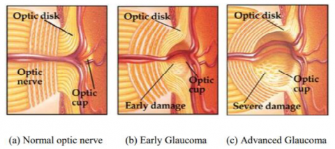
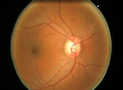
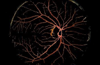
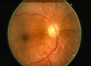
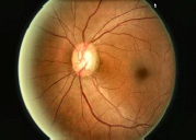
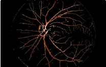
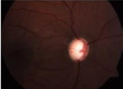
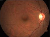
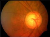
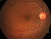
Figure 1. Progressive glaucoma
When observed through the pupil, the optic nerve's appearance has been characterized by the cupping of the optic nerve. The cup appears to be larger with the loss of the nerve fibers arising from increased IOP. In the healthy condition shown in Figure 1(a), the cup appears to be small as many nerve fibers travel through it. However, as shown in Figure 1(b) and Figure 1(c), as glaucoma progresses from an early to advanced stage, the cup progressively enlarges with increased damage to the optic nerve [5]. The amount of cupping is referred to as the CDR. The extent of nerve fibers can be quantified with CDR.
In a healthy eye, the CDR is less than 0.5. This numerical representation denotes the extent to which the optic cup occupies half of the optic disc's diameter, known as the ONH (optic nerve head). Glaucoma affected eyes have more cupping towards the vertical direction than the horizontal [6]. Shifting in the position of a blood vessel in the optic disc region along with cupping is also an indication of Glaucoma. In the advanced stage, the nerve fibers are damaged and the optic disc region is fully cupped leading to loss of vision. Additionally, macular degeneration, a degenerative eye disease affecting the macula responsible for sharp visual acuity, can also be present [7]. By utilizing the appropriate image processing algorithm, it is possible to obtain accurate and automated measurements of both the optic disc and optic cup diameters from a fundus image.
The presence of elevated blood sugar levels in individuals with diabetes plays a role in the emergence of systemic degenerative conditions, namely diabetic retinopathy, glaucoma, and cardiovascular diseases. These conditions are characterized by a shared factor of high blood pressure. Glaucoma and cardiac disorders result from the dysfunction of blood vessels, leading to diminished blood flow, inadequate oxygenation, and insufficient nutrient delivery to both the optic nerve and the heart.
Ischemia, which refers to an inadequate blood supply, plays a role in the development of both glaucoma and cardiac diseases. Ischemic damage and elevated oxidative stress are notable contributors to the progression of these conditions. Diabetic autonomic neuropathy affects the regulation of blood flow in several organs, including the eyes and heart. This neuropathy causes damage to the nerves responsible for controlling internal organs, resulting in distractions in heart rate, blood pressure, vision, and bladder function. This shared attribute between glaucoma and cardiac risk emphasizes their association.
In a Glaucoma screening program, patients usually undergo a manual examination by an ophthalmologist. The screening techniques employed for Glaucoma include Tonometry, Pachymetry, Gonioscopy, Perimetry, and Ophthalmoscopy. Ophthalmoscopy, among these techniques, plays a vital role in Glaucoma screening. To help ophthalmologists handle a larger number of patients without compromising the quality of examination, an alternative screening method is suggested as a replacement for the manual procedure. The new screening technique involves the computer-aided diagnosis of the retinal disorder. It enhances quality and effectiveness [8].
Computer-aided method of Glaucoma detection supports in screening on a huge scale and is based on the retinal fundus image analysis [9]. The screening procedure initiates by discerning patients who exhibit no Glaucoma-related irregularities, and solely those instances that the system identifies as potentially indicating Glaucoma necessitate subsequent evaluation by an ophthalmologist. This screening methodology proficiently alleviates the burden on healthcare providers, augmenting the effectiveness of broad-scale screening. Moreover, this approach serves as a means to tackle the challenge of inadequate availability of proficient personnel [10].
Image segmentation is an essential part of image processing that partitions the image into its constituent with features such as grey level, spectrum, texture and color. Image segmentation is to partition the image into disjoint regions with attributes such as intensity and tone. Through image segmentation, each pixel in an image is assigned a specific label based on shared visual characteristics among pixels with similar labels [11]. Segmenting complex images poses a significant challenge in image processing.
The second approach depends on predefined criteria upon which the image gets segmented. In a decision-oriented application, image segmentation accurately classifies the pixels of the picture. It partitions an input image into multiple distinct regions where there is a significant similarity among pixels within each region and a noticeable contrast between adjacent regions. It is employed in a variety of fields, including pattern recognition, image processing, and healthcare [12]. Multiple techniques are available for segmenting images for extracting the reliable features, such as threshold-based methods, edge-based methods, cluster-based methods, and neural network-based methods.
Unsupervised learning problems, particularly clustering, hold substantial significance. Clustering is a technique employed to divide data into a number of groups. The incorporation of bio-inspired approaches has a huge impact on performance improvement [13]. This research places emphasis on the detection of Glaucoma, as it has been identified as a significant contributor to cardiovascular disease. This necessitates the early-stage detection of the Glaucoma. The incidence of diabetes is higher nowadays, and diabetes has diverse risk factors. The drive to investigate the identification of glaucoma and its association with the risk of cardiovascular disease in individuals with diabetes mellitus has led researchers from diverse disciplines to conduct comprehensive studies in this specific domain. Given that elevated intraocular pressure is known to cause damage to the optic nerve, and considering the focus of this research on diabetes mellitus, which is associated with increased blood pressure, it becomes evident that the abnormalities observed in glaucoma serve as a significant indicator of cardiovascular disease.
The main goal of this research is to employ the Genetically Optimized Neural Network (GONN) to classify glaucoma fundus images, thereby identifying abnormalities that act as the indicator of the risk of cardiovascular disease. By incorporating wavelet transformation and employing a bio-inspired genetic algorithm, the system captures intricate image details, resulting in a notable enhancement in performance. The structure of the article is as follows: Section 2 presents the related work, Section 3 describes the proposed methodology, Section 4 discusses the results, and Section 5 concludes the article.
Studies have primarily focused on investigating various invasive and non-invasive techniques for detecting and classifying glaucoma. Additionally, researchers have devoted their efforts in exploring the association between glaucoma and cardiovascular disease, thereby advancing the current knowledge in this research domain.
Glaucoma detection was a demanding process that needs knowledge and practice. Convolutional Neural Networks (CNN) schemes were introduced by Gómez-Valverde et al. [14] to provide the influence of relevant factors. The performance of the CNN-based system surpassed that of human evaluators when incorporating integrated images from patients' clinical histories [14]. The glaucoma recognition technique termed Gray Wolf Optimized Neural Network (GWO-NN) was introduced by Jerith and Kumar [15] to identify the presence or absence of disease in patient. In their study, An et al. [16] employed input photographs to accomplish transfer learning on the CNN that is in the convolutional neural network. A grayscale fundus picture of the optic disc was used.
Glaucoma has been recognized as a significant cause of blindness. The early detection prevented the patients from permanent blindness. Fundus photography revolutionized the ophthalmology area and visualized the optic disc structure. An automated diagnostic system was introduced by Gour and Khanna [17] depending on the fundus images for glaucoma disease detection.
In their study, Rehman et al. [18] introduced a multi-parametric approach for detecting and localizing the optic disc in retinal fundus images. The method leveraged region-based statistical and textural features to accomplish this task. To select discriminative features, the mutual information criterion was employed alongside Support Vector Machine, Random Forest (RF), AdaBoost, and RusBoost algorithms. They used phylogenetic diversity indices in retinal pictures to offer an autonomous glaucoma diagnosis method known as the deep learning approach with the investigation of texture features. An image was acquired from databases through training a convolutional neural network for optical disc segmentation. After conducting the feature extraction procedure from the RGB channels and grey levels, it was imperative to carry out the elimination of blood vessels. The retrieved qualities were based on phylogenetic diversity indices that measured textural properties. An extensive range of machine learning and deep learning techniques have been developed to proficiently detect and diagnose instances of glaucoma.
Shanmugam et al. [19] used phylogenetic diversity indices in retinal pictures to offer an autonomous glaucoma diagnosis method known as deep learning approach with investigation of texture features. By training a convolutional neural network specifically for optical disc segmentation, an image was obtained from databases. After conducting the feature extraction procedure from the RGB channels and grey levels, it was imperative to carry out the elimination of blood vessels. The retrieved qualities were based on phylogenetic diversity indices that measured textural properties. Various machine learning and deep learning techniques have been developed to accurately identify glaucoma with high effectiveness. Existing approaches face difficulty in learning that is rectified using segmentation and pruning in the proposed approach.
The system describes a skin cancer detection model that achieves high accuracy by combining various deep learning algorithms and machine learning algorithms. The model incorporates a GF filter for the elimination of noise, utilizes local binary patterns and Inception V3 for feature extraction, and employs LSTM for classification purposes. The model was validated on a dataset of 1000 images and cross-validated on additional images, showing promising results that might deliver a convenient tool for oncologists [20]. Fast random forest (FRF) algorithm is employed to train a supervised machine learning model to identify and classify melanoma defects in skin lesion images The FRF algorithm was used to highlight anomalous areas of the skin that follow the Allen-Spitz criteria for melanoma. The results show that the FRF algorithm achieved a level of precision that could make it a convenient tool to aid dermatopathologists in the challenging analysis of malignant melanoma [21].
Within this research paper, an innovative CNN architecture is introduced specifically for the recognition of multispectral images. This architecture demonstrates a reduced parameter count in comparison to renowned designs like ResNet and DenseNet. Remarkably, the proposed architecture exhibits superior performance over a similar network trained on RGB images and effectively mitigates the uncertainty associated with class predictions. To validate its efficacy, the study thoroughly assesses the accuracy of the network's predictions against the corresponding images [22].
This paper presents a method for predicting human gaze patterns in videos by utilizing a deep neural network (DNN). The proposed method undergoes training on an extensive dataset comprising eye-tracking data and video frames. It is able to accurately predict gaze patterns on new video frames. The approach is evaluated on several benchmark datasets and achieves state-of-the-art performance, demonstrating its potential applications in areas such as video compression, video summarization, and content analysis [23].
3.1 Glaucoma analysis using deep learning approach
FCM segmentation in the study is motivated by its suitability for image segmentation, specifically in the context of glaucoma fundus images. The region of interest in glaucoma fundus images pertains to the deformation of the structure located behind the optic nerve, commonly known as the cupping ratio. This method is appropriate for the identification and extraction of key features within the images and facilitates subsequent analysis and classification tasks.
Additionally, the utilization of wavelet transformation and genetic algorithm is used for network pruning and classification of the glaucoma fundus images. These methods are considered suitable for achieving the research goals as they facilitate feature pruning by eliminating less significant contributions for subsequent steps. Consequently, they allow for a reduction in network complexity while enhancing the efficiency and accuracy of classification tasks. To accomplish feature pruning, the application of Minkowski Sammon mapping is employed as it effectively captures the intricate 3D structural details present within the fundus image. The wavelet transformation aids in extracting relevant features from the images, while the genetic algorithm optimizes the network structure by iteratively selecting and refining the most informative features.
Overall, the chosen methods contribute to the research goals by enabling effective image segmentation, network pruning and classification of glaucoma fundus images.
In FCM segmentation data points can gradually join clusters through the use of fuzzy cluster analysis, which uses degrees between [0,1]. The ability to specify that the data points might fit more than one cluster is made possible by this. FCM still attempts to divide the data set while using an objective function that must be minimized. Values ranging from 0 to 1 are assigned to the elements in the membership matrix U. However, Eq. (1) states that the total of a data point's degrees of belongingness to entire clusters is permanently equivalent to the value 1.
$\sum_{\mathrm{i}=1}^{\mathrm{c}} \mathrm{u}_{\mathrm{ij}}=1, \forall \mathrm{j}=1,2, \ldots . \mathrm{n}$ (1)
Eq. (2) is the generalized form of the objective function which is used for FCM.
$J\left(U, c_1, c_2, \ldots \ldots, c_c\right)=\sum_{i=1}^c J_i=\sum_{i=1}^c \sum_{j=1}^n u_{i j}^m d_{i j}^2$ (2)
The value of $u_{i j}$ ranges between 0 and 1 , where $u_{-} i j$ represents the membership degree of data point $\mathrm{j}$ in fuzzy group i. The Euclidean distance, denoted as $d_{i j}=\left\|c_i-x_j\right\|$, measures the distance between the cluster center $c_i$ of fuzzy group $i$ and the data point $x_j$. Additionally, $m$, which is a weighting component, takes on values between 1 and infinity.
Essential situations to attain its minimum are given in Eq. (3).
$c_i=\frac{\sum_{j=1}^n \quad u_{i j}^m \quad x_j}{\sum_{j=1}^n \quad u_{i j}^m}$ (3)
and
$\mathrm{u}_{\mathrm{ij}}=\frac{1}{\sum_{\mathrm{k}=1}^{\mathrm{c}}\left(\frac{\mathrm{d}_{\mathrm{ij}}}{\mathrm{d}_{\mathrm{kj}}}\right)^{2 /(\mathrm{m}-1)}}$ (4)
The algorithm iteratively goes through the first two requirements until no more progress is made. The following stages are used by FCM in batch mode operation to identify the cluster centres and the membership matrix U.
Algorithm 1. FCM for Segmentation
Step 1.Initialization of U and checking the constraint in Eq. (1).
Step 2.Use Eq. (2). to determine the c fuzzy cluster centres.
Step 3.Use Eq. (3). to compute the goal function. Stop if the improvement over the previous iteration is either below a specific threshold or it is below a given tolerance value.
Step 4.Create a new U by applying Eq. (4). Achieve Step 2.
Drawing inspiration from biological neural networks, artificial neural networks (ANNs) are intricate structures that operate in a highly parallel manner, collaborating harmoniously to address an extensive range of research domains. These structures consist of a large number of small processing elements termed neurons or nodes connected by connection strengths called synapses or weights. Both the number of neurons as well as values of weights can be varied with the help of some rules to find a solution to a problem.
Artificial Neural Networks have more than one layer. The layers positioned between the input and output layers are commonly referred to as the "hidden layers". These hidden layers in the artificial neural networks are also known as multi-layer artificial neural networks. The signals stemming from the input layer are transmitted to the successive hidden layers, persisting in this progression until reaching the ultimate layer, recognized as the output layer. The signals are not passed in the reverse direction from the output layer towards the input. Due to this property of a network, these networks are termed Multi-Layer Feedforward Artificial Neural Networks [24].
The FCM-based approaches are refined by introducing spatial limitations into the goal functionality of FCM. These approaches are used for intensity inhomogeneity correction and partial volume segmentation. Refined and upgraded FCM classification techniques have been employed to expedite the picture segmentation process and to address the intensity inhomogeneity during segmentation. Similar to the other methods, the multi-threshold segmentation assessment was the criterion for the categorization and identification of the illness. The results achieved by this proposed method are better compared to the previously described methods. Table 1 below compares the accuracy of the proposed technique.
Table 1. Efficiency of segmentation
|
S. No |
Accuracy Parameter |
Efficiency |
|
|
Multi-thresholding Segmentation |
FCM Segmentation |
||
|
1 |
Sensitivity |
83 |
98.71 |
|
2 |
Specificity |
61 |
99.64 |
3.2 Convolutional layer
The convolutional layer applies convolutional operations to the input using multiple filters, which are then subjected to an activation function represented by ψ in Eq. (5).
$\begin{gathered}\forall \mathrm{n} \in\left[1,2, \ldots, \mathrm{n}_{\mathrm{C}}^{[\mathrm{ll}]}\right]: \\ \operatorname{conv}\left(\mathrm{a}^{[1-1]}, \mathrm{K}^{(\mathrm{n})}\right)_{\mathrm{x}, \mathrm{y}}=\Psi^{[1]}\left(\sum_{\mathrm{i}=1}^{\mathrm{n}_{\mathrm{H}}^{[\mathrm{n}-1]}} \sum_{\mathrm{j}=1}^{\mathrm{n}_{\mathrm{W}}^{[l-1]}} \sum_{\mathrm{k}=1}^{\mathrm{n}_{\mathrm{C}}^{[l-1]}} \mathrm{K}_{\mathrm{i}, \mathrm{j}, \mathrm{k}}^{(\mathrm{n})} \mathrm{a}_{\mathrm{x}+\mathrm{i}-1, \mathrm{y}+\mathrm{j}-1, \mathrm{k}}^{[l-1]}+\mathrm{b}_{\mathrm{n}}^{[1]}\right) \\ \operatorname{dim}\left(\operatorname{conv}\left(\mathrm{a}^{[1-1]}, \mathrm{K}^{(\mathrm{n})}\right)\right)=\left(\mathrm{n}_{\mathrm{H}}^{[1]}, \mathrm{n}_{\mathrm{W}}^{[l]}\right)\end{gathered}$ (5)
Thus by Eq. (6):
$\begin{gathered}\mathrm{a}^{[1]}=\left[\psi^{[1]}\left(\operatorname{conv}\left(\mathrm{a}^{[1-1]}, \mathrm{K}^{(1)}\right)\right), \psi^{[1]}\left(\operatorname{conv}\left(\mathrm{a}^{[1-1]}, \mathrm{K}^{(2)}\right)\right), \ldots, \psi^{[1]}\left(\operatorname{conv}\left(\mathrm{a}^{[1-1]}, \mathrm{K}^{\left(\mathrm{n}_{\mathrm{C}}^{[1)}\right)}\right)\right)\right] \\ \operatorname{dim}\left(\mathrm{a}^{[1]}\right)=\left(\mathrm{n}_{\mathrm{H}}^{[1]}, \mathrm{n}_{\mathrm{W}}^{[1]}, \mathrm{n}_{\mathrm{C}}^{[1]}\right)\end{gathered}$ (6)
With Eq. (7):
$\begin{aligned} \mathrm{n}_{\mathrm{H} / \mathrm{w}}^{[1]}= & {\left[\frac{\mathrm{n}_{\mathrm{H} / \mathrm{w}}^{(1-1)}+2 \mathrm{p}^{\prime l}-\mathrm{f}^{\mathrm{ll}}}{\mathrm{s}^{\mathrm{ll}}}+1\right] ; \mathrm{s}>0 } \\ = & \mathrm{n}_{\mathrm{H} / \mathrm{w}}^{[1-1]}+2 \mathrm{p}^{[1]}-\mathrm{f}^{[1]} ; \mathrm{s}=0 \\ & \mathrm{n}_{\mathrm{C}}^{[1]}=\text { filters count }\end{aligned}$ (7)
Learned parameters of $\mathrm{l}^{\text {th }}$ layer are:
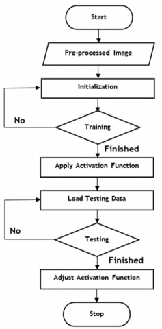
Figure 2. Overall process of training and testing
3.3 Pooling layer
As mentioned earlier, the pooling layer performs down sampling on the input's characteristics, as described in Eqs. (8). and (9), with the objective of reducing the number of channels.
$\begin{gathered}a_{x, y, z}^{[l]}=\operatorname{pool}\left(a^{[1-1]}\right)_{x, y, z} \\ =\phi^{[l]}\left(\left(a_{x+i-1, y+j-1, z}^{[l-1]}\right)_{(i, j) \in\left[1,2, \ldots, f^{[l]}\right]^2}\right) \\ \operatorname{dim}\left(a^{[l]}\right)=\left(n_H^{[l]}, n_W^{\left[l_1\right)}, n_C^{[l]}\right)\end{gathered}$ (8)
$\begin{gathered}n_{H / W}^{[l]}=\left[\frac{n_{H / W}^{[l-1]}+2 p^{[l]}-f^{[l]}}{s^{[l]}}+1\right] ; S>0 \\ =n_{H / W}^{[l-1]}+2 p^{[l]}-f^{[l]} ; s=0 \\ n_C^{[l]}=n_C^{[l-1]}\end{gathered}$ (9)
For the pooling layer, there are no parameters to learn.
For the pooling layer, there are no parameters to learn. Figure 2 represents the overall processing of training the given glaucoma image to identify the abnormalities and testing for identifying the cardiac risk prediction of the provided images.
The glaucoma images are transformed using wavelet transformation. Then the gradual genetic search is applied to the images for making the image segmentation. The pruning of the images is done for the perfect segmentation to yield the expected output. During the training phase, the activation function is employed on 70% of the images to discern between abnormal and normal ones. To assess the performance of the trained model, the remaining 30% of the images are utilized, and the activation function is adjusted correspondingly.
3.4 Fully connected layer
The fully connected layer consists of a reduced quantity of neurons, each of which can only output one vector at a time. Taking into account that the jth node of the ith layer is provided by Eq. (10).
$z_j^{[i]}=\sum_{l=1}^{n_{i-1}} w_{j, l}^{[i]} a_l^{[i-1]}+b_j^{[i]}\rightarrow a_j^{[i]}=\psi^{[i]}\left(z_j^{[i]}\right)$ (10)
$\mathrm{a}^{[\mathrm{i}-1]}$ represents the pooling layer also referred to as the convolution layer resulting with the dimensions $\left(n_{\mathrm{H}}^{[\mathrm{i}-1]}, \mathrm{n}_{\mathrm{W}}^{[\mathrm{i}-1]}, \mathrm{n}_{\mathrm{C}}^{[\mathrm{i}-1]}\right)$. To incorporate it into the fully connected layer, the tensor undergoes a flattening process, resulting in a vector of dimensions: $\left(\mathrm{n}_{\mathrm{H}}^{[\mathrm{i}-1]} \times \mathrm{n}_{\mathrm{W}}^{[\mathrm{i}-1]} \times \mathrm{n}_{\mathrm{C}}^{[\mathrm{i}-1]}, 1\right)$, thus by Eq. (11):
$n_{i-1}=n_H^{[i-1]} \times n_W^{[i-1]} \times n_C^{[i-1]}$ (11)
The acquired parameters of the $l^{t h}$ layer consist of bias and weight.
Pruning neural networks is crucial for lowering deep neural networks' extremely high compute costs. By employing custom-designed rules and a predetermined pruning ratio (PR), traditional network pruning approaches decrease the network, but because they do not take into account the variety of channels between different layers, the resulting reduced model is not optimal.
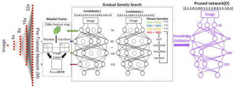
This study proposes a multi-stage genetic optimization approach for network pruning, which is characterized as a genetically modified wavelet search method. An essential concept is to encrypt each channel of the relevant network and segment it into diverse search regions aligned with the functional convolutional layers, progressing from specific to abstract. To identify the most representative and distinguishing channels at each layer and consistently refine the system, it employs a fitness function that utilizes aggregated wavelet channels while also pruning them. Figure 3 provides an introduction to the genetic technique for neural networks.
Figure 3. Enhancing network pruning with genetic wavelet transform
Table 2. Comparison of pre-processing and segmentation
|
Pre-Processing |
Segmentation |
|
|
Glaucoma Positive |
Glaucoma Negative |
|
The occurrences and features in the given image are merged, and the resulting data is fed into the input layer for predictive analytics. To preprocess the data, a Gaussian kernel map reduction model is employed. Subsequently, the Minkowski sammon mapping with the steepest descent is utilized to identify significant characteristics and eliminate irrelevant elements. The regression function is then used to look at output classes and similarity values after that. When labelling data, it uses a binary step activation function to label each class of data separately. The output layer is where categorization results are obtained. To achieve accurate classification results with a lower error rate, the GONN algorithm is used.
This section discusses the result acquired from the classification of glaucoma images; the results were compared with existing techniques. The oct eye scan is considered in this research where 70% is utilized in testing and 30% is utilized in training. The results were investigated in terms of Accuracy, F1-Score, Cohen Kappa Score, and MSE. The results were compared with existing techniques namely ANN, Naïve Bayes, Multi-Layer Perceptron, Ensemble Method, K-Nearest Neighbour, and Decision Tree. The pre-processing and segmentation of the images are performed using a Gaussian filter and FCM (Fuzzy C-Means) techniques, respectively. Table 2. Illustrates the pre-processed image where the unwanted noise and other information are removed. The fine edges and needed regions are highlighted using segmentation that utilizes the FCM technique. To reduce noise and blur specific areas of an image, a low-pass filter known as the Gaussian filter is employed. The effectiveness of the low-pass function may then be modified by adjusting the filter's width.
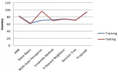
Figure 4. Graphical representation of accuracy
Accuracy is one of the parameters for assessing classification techniques. Any categorization effort must include an accuracy evaluation for assessing the effectiveness of the proposed model. The achieved accuracy of the proposed technique is presented in Table 3, while Figure 4 visually illustrates the results. The accuracy is estimated using Eq. (12).
Accuracy $=\frac{T_P+T_N}{T_P+T_N+F_P+F_N}$ (12)
The proposed approach demonstrated improved classification accuracy for both training and testing, as indicated in Table 3 and Table 4. This model has acquired 94.43% in training accuracy and 93.79% in testing accuracy, which is greater than the other models that have been examined. Figure 4 depicts the correlation between the accuracy of various algorithm types during both the training and testing phases.
Table 3. Training and testing of accuracy
|
Algorithm |
Training |
Testing |
|
ANN |
83.2 |
81.57 |
|
Naïve Bayes |
62.53 |
60.71 |
|
Multi-Layer Perceptron |
71.03 |
96.19 |
|
Ensemble Method |
72.14 |
69.38 |
|
K-Nearest Neighbour |
74.92 |
73.87 |
|
Decision Tree |
71.43 |
70.69 |
|
GONN |
94.43 |
93.79 |
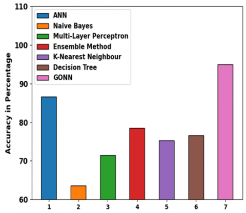
Table 4. Comparison of accuracy
|
Algorithm |
Accuracy |
|
ANN |
86.67 |
|
Naïve Bayes |
63.64 |
|
Multi-Layer Perceptron |
71.43 |
|
Ensemble Method |
78.57 |
|
K-Nearest Neighbour |
75.32 |
|
Decision Tree |
76.62 |
|
GONN |
95 |
Figure 5. Comparison of accuracy
Figure 5 illustrates the accuracy of the proposed and existing techniques. The proposed genetically optimized neural network (GONN) attains 95% accuracy that is 8.33% higher than ANN, 31.36% higher than NB, 23.57% higher than MLP, 16.43% higher than EM, 19.68% higher than KNN, and 18.38% higher than DT. The average of the squared errors, or the average squared variance among the anticipated values and the real value, is what an estimator or measures (of a method for calculating an unobserved quantity). The MSE acquired from existing and proposed techniques is given in Table 4 and illustrated in Figure 5. The MSE is given in Eq. (13).
$\mathrm{MSE}=\frac{1}{\mathrm{n}} \sum_{\mathrm{i}=1}^{\mathrm{n}}\left(\mathrm{Y}_{\mathrm{i}}-\widehat{\mathrm{Y}}_{\mathrm{i}}\right)^2$ (13)
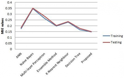
where, the count of data points is given in n, observed and forecasted values are indicated as $Y_i$ observed and forecasted values are indicated as $Y_i$ and $\widehat{Y}_i$, respectively. The observations in Table 5 shows which model have acquired better MSE values. The proposed GONN method has obtained a lower value than the other methods.
Table 5. Training and testing of MSE
|
Algorithm |
Training |
Testing |
|
ANN |
0.176 |
0.184 |
|
Naïve Bayes |
0.347 |
0.351 |
|
Multi-Layer Perceptron |
0.263 |
0.281 |
|
Ensemble Method |
0.197 |
0.201 |
|
K-Nearest Neighbour |
0.231 |
0.237 |
|
Decision Tree |
0.167 |
0.177 |
|
GONN |
0.148 |
0.151 |
Figure 6. Graphical representation of MSE
Figure 6 depicts the graphical representation of the relationship between training and testing of MSE of the different types of algorithms. Table 6 represents the comparison of MSE with the existing algorithms.
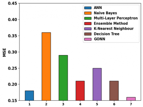
Table 6. Comparison of MSE
|
Algorithm |
MSE |
|
ANN |
0.18 |
|
Naïve Bayes |
0.36 |
|
Multi-Layer Perceptron |
0.29 |
|
Ensemble Method |
0.21 |
|
K-Nearest Neighbour |
0.25 |
|
Decision Tree |
0.21 |
|
GONN |
0.16 |
From the observation from Figure 7, the acquired MSE for GONN is minimum than the other existing techniques whereby the minimum accuracy indicates the effectiveness of the proposed technique. F1-Score is the estimation of mean values of classifies and it is statistics of single value. It is computed by Eq. (14).
$\mathrm{F} 1-\mathrm{Score}=\frac{\mathrm{TP}}{\mathrm{TP}+\frac{1}{2}(\mathrm{FP}+\mathrm{FN})}$ (14)
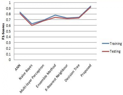
Table 7 presents the F1-Scores, indicating that the proposed model has achieved a higher F1-Score compared to alternative methods. The graph in Figure 8 represents the relationship between the training and testing of the F1 Score of the different types of algorithms.
Figure 7. Comparison of MSE
Table 7. Training and testing of F1-Score
|
Algorithm |
Training |
Testing |
|
ANN |
0.83 |
0.81 |
|
Naïve Bayes |
0.63 |
0.60 |
|
Multi-Layer Perceptron |
0.69 |
0.68 |
|
Ensemble Method |
0.78 |
0.74 |
|
K-Nearest Neighbour |
0.73 |
0.72 |
|
Decision Tree |
0.74 |
0.73 |
|
GONN |
0.94 |
0.92 |
Figure 8. Graphical representation of F1-Score
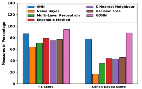
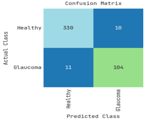
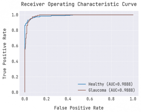
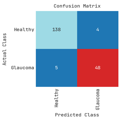
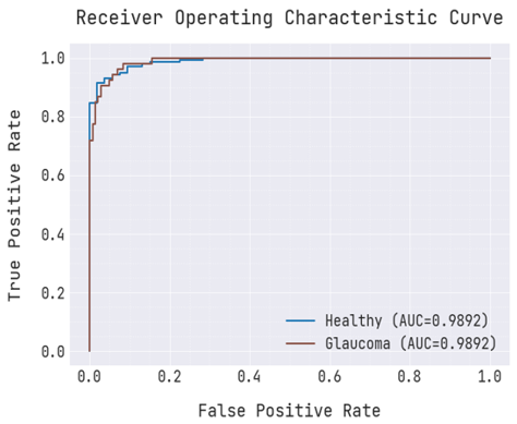
After closely examining Figure 9, it becomes apparent that the proposed methodology demonstrates favorable outcomes in both F1-Score and Cohen Kappa Score. In this research, by evaluating all the approaches such as ANN, Naïve Bayes, Multi-layer Perceptron, Ensemble Method, K-Nearest Neighbour, and Decision Tree, the proposed model has attained enhanced results in both the training and testing stages. The trade-off between sensitivity and specificity is indicated by the receiver operating characteristic curve (ROC curve). The classifier performance is investigated using a matrix called the Confusion matrix. Figure 10, depicts the ROC curve and Confusion matrix of the GONN technique. Glaucoma mostly occurs in the patient with diabetes and the severity of glaucoma may lead to heart-related issues. The retina vasculature, or configuration of blood vessels in the back of the eye, is directly related to heart health. This implies that conditions affecting the eyes might have a direct impact on heart and blood vessel health. This research focuses on the identification of glaucoma and the proposed approach attains effective accuracy. Table 8 represents the comparison of F1-Score and Cohen Kappa Score with the existing algorithms.
Table 8. Comparison of F1-Score and Cohen kappa statistics
|
Algorithm |
F1 Score |
Cohen Kappa Score |
|
ANN |
0.87 |
0.78 |
|
Naïve Bayes |
0.64 |
0.17 |
|
Multi-Layer Perceptron |
0.71 |
0.35 |
|
Ensemble Method |
0.79 |
0.44 |
|
K-Nearest Neighbour |
0.75 |
0.43 |
|
Decision Tree |
0.77 |
0.46 |
|
GONN |
0.9414 |
0.8827 |
Figure 9. Comparison of F1-Score and Cohen kappa statistics
a. Confusion Matrix-Training
b. ROC Curve -Training
c. Confusion Matrix-Testing
d. ROC Curve – Testing
Figure 10. Confusion matrix and ROC curve
The proposed approach incorporates pruning into deep learning techniques, specifically utilizing genetic algorithm (GA) and wavelet transformation to prune network channels. This post-processing technique effectively removes unnecessary parameters from neural networks while minimizing performance impact. Glaucoma detection using computational technologies at an early stage is crucial for diagnosis and management. The study reveals that glaucoma abnormalities are associated with an elevated risk of cardiovascular disease, as supported by the ground truth data. The findings of this study highlight the significance of glaucoma diagnosis in identifying potential cardiac problems and the risk of diabetes, ultimately impacting cardiovascular disease management. By addressing the challenges of achieving uniform training in deep neural networks, the proposed approach offers a solution to overcome this obstacle. The proposed approach, referred to as GONN (Genetically optimized Neural Network), outperforms existing methodologies with an impressive accuracy of 95%. In future work, the approach can be extended by incorporating additional deep learning techniques and integrating cardiovascular disease-related medical data. This future extension would enable more accurate predictions of cardiovascular disease occurrence among individuals classified as having abnormal glaucoma.
[1] Sarhan, A., Rokne, J., Alhajj, R. (2019). Glaucoma detection using image processing techniques: A literature review. Computerized Medical Imaging and Graphics, 78: 101657. https://doi.org/10.1016/j.compmedimag.2019.101657
[2] Barros, D., Moura, J.C., Freire, C.R., Taleb, A.C., Valentim, R.A., Morais, P.S. (2020). Machine learning applied to retinal image processing for glaucoma detection: review and perspective. Biomedical Engineering Online, 19(1): 1-21. https://doi.org/10.1186/s12938-020-00767-2
[3] Khunger, M., Choudhury, T., Satapathy, S.C., Ting, K.C. (2019). Automated detection of glaucoma using image processing techniques. Emerging Technologies in Data Mining and Information Security: Proceedings of IEMIS 2018, 3: 323-335. https://doi.org/10.1007/978-981-13-1501-5_28
[4] Tamilvizhi, T., Surendran, R., Anbazhagan, K., Rajkumar, K. (2022). Quantum behaved particle swarm optimization-based deep transfer learning model for sugarcane leaf disease detection and classification. Mathematical Problems in Engineering, 2022. https://doi.org/10.1155/2022/3452413
[5] Soorya, M., Issac, A., Dutta, M.K. (2018). An automated and robust image processing algorithm for glaucoma diagnosis from fundus images using novel blood vessel tracking and bend point detection. International Journal of Medical Informatics, 110: 52-70. https://doi.org/10.1016/j.ijmedinf.2017.11.015
[6] Shanthamalar, J.J., Ramani, R.G. (2021). A novel approach for glaucoma disease identification through optic nerve head feature extraction and random tree classification. International Journal of Computing and Digital Systems, 10: 675-688. http://dx.doi.org/10.12785/ijcds/100164
[7] Sahu, S., Singh, H.V., Kumar, B., Singh, A.K., Kumar, P. (2019). Image processing based automated glaucoma detection techniques and role of de-noising: a technical survey. Handbook of Multimedia Information Security: Techniques and Applications, 359-375. https://doi.org/10.1007/978-3-030-15887-3_16
[8] Soltani, A., Battikh, T., Jabri, I., Lakhoua, N. (2018). A new expert system based on fuzzy logic and image processing algorithms for early glaucoma diagnosis. Biomedical Signal Processing and Control, 40: 366-377. https://doi.org/10.1016/j.bspc.2017.10.009
[9] Ogudo, K.A., Surendran, R., Khalaf, O.I. (2023). Optimal artificial intelligence based automated skin lesion detection and classification model. Computer Systems Science & Engineering, 44(1): 693-707. https://doi.org/10.32604/csse.2023.024154
[10] Deperlioglu, O., Kose, U., Gupta, D., Khanna, A., Giampaolo, F., Fortino, G. (2022). Explainable framework for Glaucoma diagnosis by image processing and convolutional neural network synergy: analysis with doctor evaluation. Future Generation Computer Systems, 129: 152-169. https://doi.org/10.1016/j.future.2021.11.018
[11] Thanarajan, T., Alotaibi, Y., Rajendran, S., Nagappan, K. (2023). Improved wolf swarm optimization with deep-learning-based movement analysis and self-regulated human activity recognition. AIMS Mathematics, 8(5): 12520-12539.
[12] Ghani, F., Sattar, U., Narmeen, M., Wazir Khan, H., Mehmood, A. (2021). A methodology for glaucoma disease detection using deep learning techniques. International Journal of Computing and Digital System, 11(1): 401-411. https://dx.doi.org/10.12785/ijcds/110133
[13] Jeevika Tharini, V., Vijayarani, S. (2020). Bio-inspired High-Utility Item Framework based Particle Swarm Optimization Tree Algorithms for Mining High Utility Itemset. In Advances in Computational Intelligence and Informatics: Proceedings of ICACII 2019, Hyderabad, India, pp. 265-276. https://doi.org/10.1007/978-981-15-3338-9_31
[14] Gómez-Valverde, J.J., Antón, A., Fatti, G., Liefers, B., Herranz, A., Santos, A., Ledesma-Carbayo, M.J. (2019). Automatic glaucoma classification using color fundus images based on convolutional neural networks and transfer learning. Biomedical Optics Express, 10(2): 892-913. https://doi.org/10.1364/BOE.10.000892
[15] Jerith, G.G., Kumar, P.N. (2020). Recognition of Glaucoma by means of gray wolf optimized neural network. Multimedia Tools and Applications, 79(15-16): 10341-10361. https://doi.org/10.1007/s11042-019-7224-1
[16] An, G., Omodaka, K., Hashimoto, K., Tsuda, S., Shiga, Y., Takada, N., Nakazawa, T. (2019). Glaucoma diagnosis with machine learning based on optical coherence tomography and color fundus images. Journal of Healthcare Engineering. https://doi.org/10.1155/2019/4061313
[17] Gour, N., Khanna, P. (2021). Multi-class multi-label ophthalmological disease detection using transfer learning based convolutional neural network. Biomedical Signal Processing and Control, 66: 102329. https://doi.org/10.1016/j.bspc.2020.102329
[18] Rehman, Z.U., Naqvi, S.S., Khan, T.M., Arsalan, M., Khan, M.A., Khalil, M.A. (2019). Multi-parametric optic disc segmentation using superpixel based feature classification. Expert Systems with Applications, 120: 461-473. https://doi.org/10.1016/j.eswa.2018.12.008
[19] Shanmugam, G., Thanarajan, T., Rajendran, S., Murugaraj, S.S. (2023). Student psychology based optimized routing algorithm for big data clustering in IoT with MapReduce framework. Journal of Intelligent & Fuzzy Systems, 44(2): 2051-2063. https://doi.org/10.3233/JIFS-221391
[20] Cazzato, G., Massaro, A., Colagrande, A., Lettini, T., Cicco, S., Parente, P., Nacchiero, E., Lospalluti, L., Cascardi, E., Giudice, G., Ingravallo, G., Resta, L., Maiorano, E., Vacca, A. (2022). Dermatopathology of malignant melanoma in the era of artificial intelligence: A single institutional experience. Diagnostics, Basel, Switzerland, 12(8): 1972. https://doi.org/10.3390/diagnostics12081972
[21] Liu, L., Awwad, E.M., Ali, Y.A., Al-Razgan, M., Maarouf, A., Abualigah, L., Hoshyar, A.N. (2023). Multi-dataset Hyper-CNN for hyperspectral image segmentation of remote sensing images. Processes, 11(2): 435. https://doi.org/10.3390/pr11020435
[22] Rajagopal, S., Thanarajan, T., Alotaibi, Y., Alghamdi, S. (2023). Brain tumor: Hybrid feature extraction based on UNet and 3DCNN. Computer Systems Science & Engineering, 45(2): 2093-2109. https://doi.org/10.32604/csse.2023.032488
[23] Alharbi, M., Rajagopal, S.K., Rajendran, S., Alshahrani, M. (2023). Plant disease classification based on ConvLSTM U-Net with fully connected convolutional layers. Traitement du Signal, 40(1): 157-166. https://doi.org/10.18280/ts.400114
[24] Vinícius dos Santos Ferreira, M., Oseas de Carvalho Filho, A., Dalília de Sousa, A., Corrêa Silva, A., Gattass, M. (2018). Convolutional neural network and texture descriptor-based automatic detection and diagnosis of glaucoma. Expert Systems with Applications, 110: 250-263. https://doi.org/10.1016/j.eswa.2018.06.010