Xingyu Ding*![]() | Wenjun Hu
| Wenjun Hu![]()
© 2023 IIETA. This article is published by IIETA and is licensed under the CC BY 4.0 license (http://creativecommons.org/licenses/by/4.0/).
OPEN ACCESS
Geological disasters, characterized by their destructive nature, pose significant threats to both human life and ecological environments. The advent of remote sensing technology has rendered hyperspectral remote sensing images an integral data source in monitoring and predicting these phenomena. However, it is noted that minor variations and detailed nuances within the images are often overlooked by traditional computer vision and deep learning techniques. Furthermore, data imbalances during the training of deep learning models have been identified as a potential hindrance to optimal performance. Recognizing these issues and the inherent unpredictability of geological disasters, an innovative approach has been developed. This approach encapsulates an optical flow-based method for enhancing the edges of geological remote sensing images, an improved geological disaster monitoring model leveraging the Isolation Forest algorithm, and an efficient implementation strategy. The suggested methods present numerous advantages, including the acceleration of computations to augment real-time monitoring of geological disasters, an enhanced capacity for handling extensive data, an improved system stability and fault tolerance, and the preservation of fundamental strengths such as linear computational complexity, unsupervised learning, and non-parametric methodologies. By synthesizing these methodological improvements and advantages, a swift, efficient, and flexible strategy for enhancing the Isolation Forest model is put forth. This research supports the development of geological disaster monitoring and early warning systems grounded in computer vision and deep learning, presenting substantial technical aid for related tasks.
machine vision, deep learning, geological disaster monitoring, geological disaster early warning
This study investigates the escalating threat of geological disasters including landslides, mudslides, and ground subsidence, which result in profound human and economic losses [1-6]. The urgency of predicting and monitoring these hazards to mitigate their impact is underscored by a consistent rise in both the annual direct economic loss and the number of fatalities attributable to these geological calamities [7, 8]. The dawn of computer vision and deep learning technologies carries potential for improving the efficiency of monitoring and warning systems tailored to these geological disasters [9, 10]. However, the existing methodologies employing these technologies exhibit significant limitations that curb progress in this critical domain.
Firstly, an evident deficiency lies in the current handling of geological remote sensing imagery by conventional computer vision and deep learning methods [11-13]. These methods tend to overlook subtle changes and detailed information within the images. However, the initiation of geological disasters often hinges on these subtle surface variations and underlying risk factors, necessitating the extraction of such intricate details for effective prediction and monitoring [14]. Unfortunately, contemporary computer vision techniques and deep learning models display restricted abilities in capturing these nuances, thereby constraining the precision of predictions and detections pertaining to geological disasters [15].
Secondly, the challenges posed by data imbalance during the training phase of deep learning models have a detrimental effect on their performance [16-19]. Geological disasters are inherently unpredictable and random, resulting in an imbalanced distribution of positive and negative samples. This disparity often leads to a bias in model training, with models typically favoring more abundant samples over those that are less frequent [20, 21]. This bias compromises the accuracy of geological disaster prediction, subsequently weakening the trustworthiness of monitoring and warning systems. Addressing this issue necessitates the development of more appropriate data processing methodologies and models.
To address these challenges, this manuscript proposes an edge enhancement method for geological remote sensing image regions predicated on optical flow fields, along with an optimized geological disaster monitoring model rooted in the Isolation Forest algorithm. The second chapter delineates the basic principle of the edge enhancement method [11-13]. Utilizing the characteristics of the optical flow field, this method effectively extracts subtle changes and detailed information within images, thereby improving the accuracy of geological disaster prediction and monitoring. The third chapter introduces the improved geological disaster monitoring model based on Isolation Forest [16-19]. By enhancing the Isolation Forest algorithm, the issue of data imbalance is effectively managed, thereby augmenting the model's performance in geological disaster prediction and monitoring.
The findings of this study bear significant theoretical and practical implications. It is anticipated that these insights will provide valuable support for technological advancement and application in the field of geological disaster monitoring and warning, thereby aiding in the reduction of the impact of geological disasters on human lives and economic development.
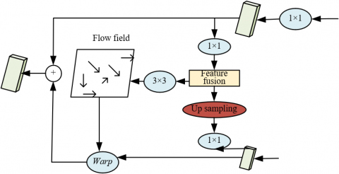
In geological disaster monitoring and early warning systems, precise detection and prediction of the boundaries of geological disaster areas are crucial. Yet, traditional computer vision methods and deep learning models often display roughness in boundary segmentation when processing geological remote sensing images. By incorporating semantic flow and edge enhancement modules, it is feasible to boost the intra-class consistency and inter-class distinctiveness of boundary pixels, thereby refining boundary precision. Edge features hold significant value in geological disaster monitoring and early warning tasks, as they can aid models in better distinguishing different types of geological disaster areas. An edge enhancement module can be built to indirectly strengthen edge features, thereby improving the model's discriminative capabilities when processing geological remote sensing images. Additionally, a geological remote sensing image region edge enhancement method based on optical flow fields can learn rich semantic flow information from feature maps of different resolutions. This aids in dynamically obtaining pixel positional relationships within the feature map, enhancing the information transfer between feature layers, and thereby improving model performance in geological disaster monitoring and early warning tasks. The architecture of the edge enhancement module is depicted in Figure 1.
The edge enhancement module for geological remote sensing images is built under the application scenario of geological disaster monitoring and early warning systems based on computer vision and deep learning research and development. Traditional bilinear interpolation upsampling methods can only deal with fixed and pre-declared feature map pixel position misalignments. However, the edge enhancement module improved by the flow alignment module can dynamically adjust the positional relationship of feature map pixels, thereby better resolving feature map pixel position misalignment issues. Since geological remote sensing images often contain complex terrain, geomorphology, and geological disaster features, the flow-aligned, edge-enhanced module can learn rich semantic flow information between feature maps of different resolutions, giving the model a stronger adaptability and better performance in complex geological remote sensing image scenarios. In semantic segmentation tasks, the recovery of smaller spatial resolution and semantically stronger feature maps is crucial. The flow-aligned, edge-enhanced module can effectively retain the information of apparent and semantic features by upsampling and skip-connection methods, thereby improving the recognition accuracy of geological remote sensing image boundaries. The dynamic positional relationship of feature map pixels is considered further in the upsampling process to enhance the model's discriminative capabilities when processing geological remote sensing images. The architecture of the flow alignment module is depicted in Figure 2.
Figure 1. Edge enhancement module
Figure 2. Flow alignment module
The input of the constructed edge enhancement module is two adjacent geological disaster sequence remote sensing image feature blocks D1 and D2 at different hierarchies, with sizes represented by H1×W1×V1 and H2×W2×V2, respectively, where H1 is greater than H2, and W1 is greater than W2. The results of 1×1 convolution operations on D1 and D2 are represented by $\bar{D}_1$ and $\bar{D}_2$. The result of performing bilinear interpolation on $\bar{D}_2$ is represented by $\bar{D}_2^1$. The flow field ∆y-1 is obtained after the concatenation and 3×3 convolution operations of $\bar{D}_2^1$ and $\bar{D}_1$. After obtaining ∆y-1, the pixel value at position (u,k) in the high-resolution feature map $\bar{D}_2^{11}$, obtained from the low-resolution feature map D2, is solved. This step requires mapping (u,k) to a specific location O in D2. The positional change from (u,k) to O is determined by the flow field ∆y-1.
$O=\frac{(u, k)+\Delta\,_{y-1}\,\,\,\,(u, k)}{2}$ (1)
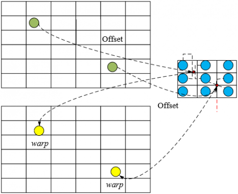
Based on the differentiable bilinear sampling mechanism in spatial transformation networks, compute the pixel value c at position (u,k) in $\bar{D}_2^{11}$ at the corresponding O position.
$C_u^v=\sum_b^H \sum_l^W I_{b l}^v M A X\left(0,1-\left|z_u^a-l\right|\right) M A X\left(0,1-\left|t_u^a-b\right|\right)$ (2)
From the above formula, it is known that the adopted interpolation mechanism is to perform linear interpolation calculations on the values at the upper left, upper right, lower left, and lower right four different positions of O, thereby achieving an update on its pixel values.
Assume that the pixel value solution for the $v$-th channel at the pixel position ($z^y_u$,$t^y_u$) in $\bar{D}_2^{11}$ is represented by $C_u^v$, the height and width of the corresponding feature map in the $z$-th channel of D2 are represented by H and W, and the pixel value of the pixel position $(b, l)$ in the v-th channel of D2 is represented by $I_{b l}^v$. The pixel position ($z^y_u$,$t^y_u$) of the high-resolution feature map to be solved is mapped to the pixel position ($z_u^a$,$t_u^a$) in the low-resolution image D2 through the flow field ∆y-1 transformation. As can be known from the above formula, when the result of $\left|t^a_u-b\right|$ or $\left|z^a_u-l\right|$ is greater than 1, $I_{b l}^v M A X() M A X()=0$, it can be considered that the pixel value of the target position in the geological disaster area is determined by the four closest pixel points to ($z_u^a$,$t_u^a$). At the same time, when the values of $\left|t^a_u-b\right|$ and $\left|z^a_u-l\right|$ are relatively small, $I_{b l}^v$ will obtain a larger weight coefficient. Based on the derivation of the above formula with respect to $I_{b l}^v$, $z_u^a$, and $t_u^a$, it is shown that the constructed edge enhancement module can adjust and correct parameters through continuous learning during the training process.
$\frac{\partial \,C_u^v}{\partial \,I_{b l}^v}=\sum_b^H \sum_l^W M A X\left(0,1-\left|z_u^a-l\right|\right) M A X\left(0,1-\left|t_u^a-b\right|\right)$ (3)
$\frac{\partial \,C_u^v}{\partial \,I_{b l}^v}=\sum_b^H \sum_l^W I_{b l}^v \operatorname{MAX}\left(0,1-\left|t_u^a-b\right|\right) \begin{cases}0, d & \left|l-z_u^a\right| \geq 1 \\ 1, d & l \geq z_u^a \\ -1, & \text { IF } \quad l<z_u\end{cases}$ (4)
In the application scenario of the research and development of a geological disaster monitoring and early warning system based on computer vision and deep learning, the improved flow alignment module can make the features after upsampling more consistent in the same object representation. This helps to improve the model's ability to discriminate different types of geological disaster areas in geological disaster monitoring and early warning tasks. By learning the relationship between adjacent feature maps to form a semantic flow, dynamically upsampling the feature maps with smaller spatial dimensions and stronger semantic expression capabilities, the obtained high-resolution features are more structurally tidy, thereby improving the recognition accuracy of geological remote sensing image edges. Compared with using only bilinear upsampling operations, the improved flow alignment module can obtain richer semantic information. This allows the model to have stronger semantic segmentation capabilities when processing geological remote sensing images, thereby achieving better performance in geological disaster monitoring and early warning tasks. These advantages make the improved flow alignment module have a higher application value in geological disaster monitoring and early warning tasks.
Current hyperspectral image geological disaster monitoring algorithms often present high computational complexity or suboptimal monitoring outcomes in practical application. The Isolation Forest algorithm, possessing linear computational complexity, yields satisfactory results when used for continuous data geological disaster monitoring tasks. However, its performance in detecting local anomalies is not ideal, with substantial false alarms and missed detections for local anomaly samples. Improvements to existing algorithms are required to enhance efficiency in handling vast remote sensing image data for geological disaster monitoring tasks.
This study, based on relative quality theory, directionally improves the original Isolation Forest algorithm. The enhanced detection sensitivity towards local geological disaster area targets, reduced risks of false alarms and missed detections, are among the improvements made. The improved Isolation Forest algorithm exhibits strong adaptability, able to deal with geological disaster monitoring tasks of various types and complexities.
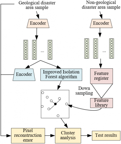
In the original Isolation Forest algorithm, the "path length" index primarily assesses global anomalies and falls short in detecting performance for local anomaly pixels. By replacing "path length" with "local relative quality", sensitivity towards local anomaly pixels is improved. The original Isolation Forest algorithm's detection performance is insufficient when dealing with local anomalies, with problems of false alarms and missed detections. The proposed improvement is expected to resolve these issues and enhance monitoring accuracy. The introduction of the concept of "local relative quality" allows the original algorithm to more accurately detect local anomaly pixels, thereby improving the accuracy of geological disaster monitoring while retaining the advantages of the original algorithm, such as linear computational complexity, unsupervised and non-parametric learning. Figure 3 shows the process of geological disaster monitoring by the proposed method.
Figure 3. Geological disaster monitoring process
Next, the definition of the relative quality anomaly score for local geological disaster area target monitoring is provided. Let's assume the Isolation Tree is represented by $Y_u$ and the relative quality of pixel z is represented by $Z L_u(z)$. It is assumed that z in the Isolation Tree $Y_u$ is represented by $Y_u(z)$ and $Y_u(z)$ in the Isolation Tree $T Y_u$ has a direct parent node represented by $\tilde{Y}_u(z)$. The number of pixels in the node is represented by $l(\cdot)$, the normalization factor by q, and the comparison of the number of pixels $l\left(\tilde{Y}_u(z)\right)$ in the leaf node where z is located with the number of pixels $l\left(Y_u(z)\right)$ in its direct parent node can yield $Z L_u(z)$:
$Z L_u(z)=\frac{l\left(\tilde{Y}_u(z)\right)}{l\left(Y_u(z)\right) \times q}$ (5)
From the above formula, it can be seen that $Z L_u(\cdot)$ is greater than 0 and less than 1. The closer the value of $Z L_u(z)$ is to 1, the higher the anomaly degree of z in its neighborhood and the higher the possibility of being a geological disaster area. The following formula gives the relative quality calculation formula for z in a forest containing y isolated trees:
$E L(z)=\frac{1}{y} \sum_{u=1}^y Z L_u(z)$ (6)
By traversing all the pixels in the geological remote sensing image based on the improved model, an anomaly degree ranking based on the local measurement of the geological disaster area target can be obtained. According to the definition of the geological disaster area target, the abnormal pixels representing the geological disaster area target should be a very small number in the whole image.
Based on this, given a geological remote sensing image containing b pixels, the abnormal score of pixel z in a forest containing y isolated trees can be calculated through the following formula:
$A_E(z, b)=1-2^{-E L(z) / v(b)}$ (7)
where, the average height of the isolated tree is represented by $c(n) v(b)$.
In order to improve the efficiency of the improved model, this study discusses the time complexity and space complexity of the Isolation Forest algorithm. Assuming that y isolated trees are required in the model training stage, each isolated tree needs q geological disaster sequence remote sensing image samples for training. The number of recursive splits is represented by $\log _2 q$, and the asymptotic time complexity of the original algorithm is represented by $Y_{T R}(q)$. The calculation,
$Y_{T R}(q)=P\left(y \cdot q \cdot \log _2 q\right)$ (8)
For a given geological disaster sequence remote sensing image containing b pixels, the asymptotic time complexity $Y_{T E}(b)$ of the original algorithm in the testing stage can be calculated by the following formula:
$Y_{T E}(b)=P\left(y \cdot b \cdot \log _2 q\right)$ (9)
The time complexity $T I(b)$ of the algorithm is provided by the following formula:
$T I(b)=P\left(y(b+q) \log _2 q\right)$ (10)
Correspondingly, the space complexity $S P(b)$ of the algorithm can be calculated by the following formula:
$S P(b)=P(y \cdot q)$ (11)
The number of pixels in the hyperspectral image and the number of pixels in the training set directly influence the time complexity of the Isolation Forest model. In geological disaster monitoring tasks, the challenge of processing a vast amount of remote sensing image data is faced. Deploying the Isolation Forest model on a large-scale distributed system can effectively utilize parallel computing resources, accelerating the computational process, and enhancing the real-time nature of geological disaster monitoring.
Furthermore, this study constructs and trains a geological disaster monitoring model, taking geological remote sensing images as an example. Assume the image height, i.e., pixel row number, is represented by G, the image width, i.e., pixel column number, by Q, and the total number of bands, i.e., pixel feature dimensions, by F. The normalized (0,1) geological remote sensing image data cube is represented by the following formula:
$Z \in \mathfrak{R}^{G \times Q \times F}$ (12)
Assume the height of the local geological disaster area target region in the image, i.e., the number of target area pixel rows, is represented by G', the width of the target area in the image, i.e., the number of target area pixel columns, by Q', and G'=G/j1, q'=q/j1. The total number of bands in the geological remote sensing image is represented by F. Divide the geological remote sensing image cube equally into j1×j1 target areas, with the kth target area denoted as:
$Z_{S U}^k \in \mathfrak{R}^{G^{\prime} \times Q^{\prime} \times F}$ (13)
Assume that the total number of pixels in the target area image is represented by B'=G'×Q', and the total number of image bands by F. Before using the improved model for geological disaster area target monitoring, each target area geological remote sensing image cube is unfolded into:
$Z_{S U}^k \in \mathfrak{R}^{B^{\prime} \times F}$ (14)
The B' pixels of this target area image can be considered as B' vectors. Hence, all pixel samples from the kth target area can be represented by the following formula:
$Z_{S U}^k=\left\{z_u\right\}_{u=1}^{B^{\prime}} \in \mathfrak{R}^F$ (15)
By partitioning the initial large field-of-view hyperspectral remote sensing image into several target areas, and unfolding the three-dimensional data cube form of hyperspectral images in each target area into a matrix, computational complexity is reduced, the speed of model training and prediction is improved, and an efficient pixel anomaly degree evaluation is facilitated using the improved Isolation Forest model. By dividing the large field-of-view hyperspectral remote sensing image into target areas and unfolding the hyperspectral images into matrices, each pixel can be effectively evaluated for its anomaly degree using the improved Isolation Forest model, enabling rapid geological disaster monitoring.
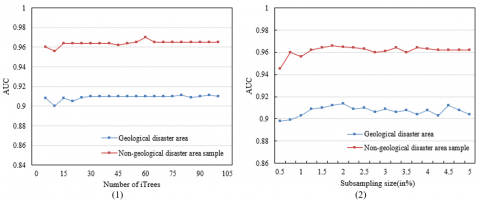
The experimental results and analysis of this study commences with an examination of the relationship between the quantity of isolated trees and the Area Under Curve (AUC) value of geological disaster monitoring results, as depicted in Figure 4. An observation from the figure reveals that as the number of isolated trees escalates from zero to fifteen, a slight reduction in AUC value is observed in both disaster-stricken and non-disaster-stricken areas. This suggests that within this range, an increase in the number of isolated trees bears a minimal effect on the AUC value of geological disaster monitoring results.
Figure 4. The influence of the number of isolated trees and the number of samples required for isolated tree training on the AUC value of monitoring results
Further analysis, when the number of isolated trees rises from fifteen to thirty, points to the disaster-stricken area's AUC value reverting to 0.908, while the AUC value of the non-disaster-stricken area slightly increases. This observation suggests that within this range, an increase in the number of isolated trees has a marginal impact on the AUC value in the disaster-stricken area but a somewhat positive effect on the AUC value in the non-disaster-stricken area.
As the isolated tree count increases from thirty to ninety, the AUC value of the disaster-stricken area experiences minor fluctuations, but the overall trend is ascendant, while the non-disaster-stricken area's AUC value remains relatively stable. This pattern suggests that within this range, an increase in the number of isolated trees has a positive impact on the disaster-stricken area's AUC value, but only a minor effect on the non-disaster-stricken area's AUC value.
An analysis of the relationship between the sample size required for isolated tree training and the AUC value of geological disaster monitoring results is also offered. It is noted that with the increase in the sample size required for isolated tree training, the AUC value of the disaster-stricken area fluctuates considerably. However, the overall trend shows an initial rise followed by a decrease. The AUC value for the disaster-stricken area reaches its peak, approximately 0.912, when the sample size is 0.03B.
For the non-disaster-stricken area, the AUC value also fluctuates with the increase in the sample size required for isolated tree training, but the overall trend remains relatively stable. The AUC value for the non-disaster-stricken area reaches its peak, approximately 0.966, when the sample size is 0.03B. Thus, 0.03B is chosen as the default sample size required for isolated tree training.
Table 1 presents a comparison of AUC values for geological disaster area classification using different algorithms. From the data presented, it is noted that the AUC values of the method used in this study outperform other algorithms for all types of geological disasters including landslides, debris flows, ground subsidence, ground fissures, and floods. This suggests the superior performance of the method used in this study in the task of geological disaster area classification.
In the case of landslides, debris flows, and ground fissures, the CNN algorithm performs well, but not as well for ground subsidence and floods. The SVM algorithm excels in ground subsidence and ground fissures but falls short in debris flows and floods. RF performs well in ground subsidence but is the weakest for debris flows. U-Net performs well for floods but poorly for ground subsidence and ground fissures. By comparing the method used in this study before and after regional edge enhancement, it is observed that AUC values for all types of geological disasters improve, suggesting the effectiveness of regional edge enhancement in improving the accuracy of geological disaster classification.
The table data presented in Table 2 provides an analytical viewpoint on the performance of different algorithms based on the AUC (Area Under the Curve) value in geological disaster zone localization tasks. Notably, the method introduced in this study displays a higher AUC value than other algorithms across landslide, debris flow, land subsidence, ground fissure, and flood geological disaster types. This indicates a superior performance of this method in geological disaster zone localization tasks. The RF (Random Forest) algorithm performs well in terms of landslides, ground fissures, and flooding, yet underperforms in detecting debris flows and land subsidence. The CNN (Convolutional Neural Networks) excels at identifying ground fissures but shows weaker performance in detecting landslides, debris flows, and land subsidence. SVM (Support Vector Machines) performs adequately in flooding scenarios, but underperforms in detecting landslides, debris flows, land subsidence, and ground fissures. U-Net performs well in debris flows and ground fissures, but underperforms in detecting landslides, land subsidence, and flooding. A comparison between the region-edge enhancement method and this study's method yields a similar conclusion - the AUC value of this method improved across all geological disaster types, thereby validating the effectiveness of region-edge enhancement in improving the accuracy of geological disaster zone localization.
Table 1. Comparison of AUC values for geological disaster area classification
|
Different algorithms |
Landslide |
Mudslide or Debris flow |
Ground subsidence |
Ground fissures |
Floods |
|
CNN |
0.945 |
0.985 |
0.891 |
0.936 |
0.954 |
|
SVM |
0.953 |
0.926 |
0.951 |
0.955 |
0.933 |
|
RF |
0.941 |
0.851 |
0.964 |
0.913 |
0.915 |
|
U-Net |
0.942 |
0.916 |
0.926 |
0.934 |
0.967 |
|
The previous method |
0.941 |
0.942 |
0.951 |
0.937 |
0.952 |
|
The method in this study |
0.958 |
0.988 |
0.978 |
0.961 |
0.975 |
|
Different algorithms |
Landslide |
Mudslide or Debris flow |
Ground subsidence |
Ground fissures |
Floods |
|
CNN |
0.895 |
0.864 |
0.846 |
0.943 |
0.862 |
|
SVM |
0.861 |
0.826 |
0.825 |
0.829 |
0.944 |
|
RF |
0.941 |
0.943 |
0.848 |
0.901 |
0.933 |
|
U-Net |
0.933 |
0.962 |
0.882 |
0.942 |
0.937 |
|
The previous method |
0.954 |
0.976 |
0.964 |
0.943 |
0.928 |
|
The method in this study |
0.968 |
0.978 |
0.978 |
0.951 |
0.955 |
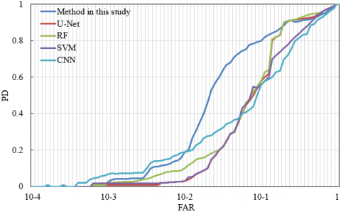
Figure 5. Standard 2D ROC (D, F) curves for different geological disaster monitoring algorithms
The standard 2D ROC (Receiver Operating Characteristic) curve of different geological disaster monitoring algorithms in Figure 5 shows the FAR (False Alarm Rate) and DR (Detection Rate) data. It is ideal to find an algorithm with a high detection rate (close to 1) and a low false alarm rate (close to 0). On the ROC curve, algorithms that are closer to the upper-left corner have superior performance. The detection rate of the method in this study gradually increases with a lower false alarm rate and significantly improves when FAR exceeds 0.6. This method generally performs well under low false alarm rate and high detection rate conditions. The detection rate of U-Net is relatively stable with a low false alarm rate and gradually increases as FAR grows, showing prominent improvement when FAR exceeds 0.6. Overall, U-Net performs well under high false alarm rate and high detection rate conditions. As the false alarm rate increases, the detection rate of RF gradually improves and becomes relatively stable when FAR exceeds 0.6. In general, RF performs adequately under moderate false alarm rate and detection rate conditions. The detection rate of SVM remains at a lower level when the false alarm rate is low, however, it significantly improves when FAR increases to 0.6. CNN has a gradually increasing detection rate under lower false alarm rate conditions, but the improvement is not significant when FAR exceeds 0.6. Overall, this method performs adequately under low false alarm rate and moderate detection rate conditions. A comprehensive analysis indicates that the method in this study exhibits the best performance under conditions of low false alarm rate and high detection rate, rendering it suitable for geological disaster monitoring applications.
Table 3. Performance comparison of different geological disaster monitoring algorithms
|
Metrics |
Method in this study |
U-Net |
RF |
SVM |
CNN |
|
Accuracy |
0.9013 |
0.8651 |
0.8235 |
0.5424 |
0.8152 |
|
Precision |
0.3845 |
0.3267 |
0.0784 |
0.0003 |
0.0018 |
|
Recall |
0.0756 |
0.1285 |
0.0465 |
0.0002 |
0.0008 |
|
F1 score |
1.2364 |
1.1582 |
0.8562 |
0.8512 |
0.8125 |
|
IoU |
5.1298 |
2.2352 |
1.7518 |
1.7582 |
2.2034 |
According to the accuracy, precision, recall, F1 score, and IoU (Intersection over Union) data of different geological disaster monitoring algorithms shown in Table 3, the performance of each algorithm can be analyzed. As can be seen from the table, the method proposed in this paper has a higher accuracy (0.9013), precision, and recall, but the F1 score (1.2364) and IoU (5.1298) indicators are relatively high. This indicates that this method performs well in terms of overall prediction accuracy, but the accuracy and coverage of detecting geological disasters need to be improved. U-Net has a higher accuracy (0.8651), precision, and recall, but the F1 score (1.1582) and IoU (2.2352) indicators are relatively low. This shows that U-Net performs well in terms of overall prediction accuracy, but there is a greater room for improvement in the accuracy and coverage of detecting geological disasters. RF has a lower accuracy (0.8235), precision, and recall, and the F1 score (0.8562) and IoU (1.7518) indicators are relatively low. This indicates that RF does not perform well in terms of overall prediction accuracy and the accuracy and coverage of detecting geological disasters. SVM has the lowest accuracy (0.5424), extremely low precision and recall, and the F1 score (0.8512) and IoU (1.7582) indicators are also relatively low. This indicates that SVM performs poorly in terms of overall prediction accuracy and the accuracy and coverage of detecting geological disasters. CNN has a lower accuracy (0.8152), extremely low precision and recall, but the F1 score (0.8125) and IoU (2.2034) indicators are relatively low. This shows that CNN needs improvement in terms of overall prediction accuracy and the accuracy and coverage of detecting geological disasters. In summary, the method proposed in this paper is relatively good in terms of accuracy, F1 score, and IoU indicators, indicating that it has better performance in overall prediction accuracy.
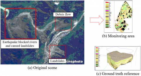
Figure 6. Monitoring example
In the geological disaster monitoring example given in Figure 6, it can be seen that the geological disaster monitoring achieves better results by enhancing the regional edges of these images. This verifies that the proposed method of regional edge enhancement for geological remote sensing images based on optical flow fields captures motion information in images by calculating optical flow fields, thereby better highlighting the edges of geological disaster areas. The improved geological disaster monitoring model based on the Isolation Forest algorithm is used to identify geological disaster areas in these enhanced images. The Isolation Forest algorithm itself has high anomaly detection performance, and this paper improves it to adapt to the scenario of geological disaster monitoring. In the experiments, this improved Isolation Forest model shows higher accuracy and stability. This further verifies that the proposed method is highly effective in improving edge clarity, detection accuracy, and computation speed. This provides strong support for geological disaster monitoring in practical applications.
This study investigates the development of a geological disaster monitoring and early warning system based on computer vision and deep learning. A regional edge enhancement method for geological remote sensing images based on optical flow fields, an improved geological disaster monitoring model based on the Isolation Forest algorithm, and a rapid implementation approach are proposed. The optical flow field-based regional edge enhancement method effectively extracts subtle changes and detailed information in images, thereby improving the accuracy of geological disaster monitoring and early warning. The improved geological disaster monitoring model based on Isolation Forest addresses data imbalance issues by optimizing the algorithm, effectively solving the data imbalance problem and enhancing the model's performance in geological disaster monitoring and early warning.
The following conclusions can be drawn from the experimental results:
This research was supported by the Hunan Provincial Natural Science Foundation of China (Grant No.: 2023JJ50339), and The Natural Science Foundation of Hunan Province, China (Grant No.: 2023JJ30212).
[1] Wu, Z., Deng, M., Chen, G., Liu, Y., Zhang, Q., Guo, L. (2023). Developing a geological disaster monitoring system based on electrical prospecting. Measurement Science and Technology, 34(4): 045902. https://doi.org/10.1088/1361-6501/aca990
[2] Fan, Z., Cao, Y., Zheng, B., Wu, B., Li, F. (2022). Geological disaster emergency decision support system based on location-based service. In 2022 International Conference on Computer Engineering and Artificial Intelligence (ICCEAI), Shijiazhuang, China, pp. 191-194. https://doi.org/10.1109/ICCEAI55464.2022.00048
[3] Zhang, J., Li, B., Chen, J., Cai, C., Li, X. (2022). Geological disaster monitoring technology along transmission line based on InSAR. In 2022 2nd International Conference on Electrical Engineering and Control Science (IC2ECS), Nanjing, China, pp. 64-67. https://doi.org/10.1109/IC2ECS57645.2022.10088150
[4] La, R.F., Liu, H., Bai, P.F., Zhang, Z.X., La, R., Han, L., Bai, P., Zhang, Z. (2022). Demand forecast of geological disaster rescue equipment based on "Scenario-Task". Geotechnical and Geological Engineering, 40(4): 2267-2290. https://doi.org/10.1007/s10706-021-02025-1
[5] Zhang, D., Feng, D. (2022). Mine geological disaster risk assessment and management based on multisensor information fusion. Mobile Information Systems, 2022: 1757026. https://doi.org/10.1155/2022/1757026
[6] Liu, Y., Zhang, J. (2022). An IoT-based intelligent geological disaster application using open-source software framework. Scientific Programming, 2022: 9285258. https://doi.org/10.1155/2022/9285258
[7] Sun, G., Sun, F., Xu, R., Guo, F., Wei, X. (2022). Application of triggered inclination monitoring microsystem base on double MEMS accelerometers in geological disaster monitoring. In 2022 International Conference on Artificial Intelligence in Everything (AIE), Lefkosa, Cyprus, pp. 117-112. https://doi.org/10.1109/AIE57029.2022.00029
[8] La, R., Lv, T., Bai, P., Zhang, Z. (2022). Research on collaborative and optimal deployment and decision making among major geological disaster rescue subjects. Geotechnical and Geological Engineering, 40(1): 57-71. https://doi.org/10.1007/s10706-021-01883-z
[9] Zhang, D., Wei, Y., Xiao, C., Wang, J., Wang, J. (2021). A multi-level dynamic database model of geological disaster emergency remote sensing monitoring. In 2021 28th International Conference on Geoinformatics, Nanchang, China, pp. 1-4. https://doi.org/10.1109/IEEECONF54055.2021.9687657
[10] Liu, G., Wang, C., Li, G., Guo, W., Zhang, Z. (2019). Application research on the remote sensing technology in geological disaster prevention and control of existing railway. Journal of Railway Engineering Society, 36(6): 23-27.
[11] Liu, Y., Wu, L. (2016). Geological disaster recognition on optical remote sensing images using deep learning. Procedia Computer Science, 91: 566-575. https://doi.org/10.1016/j.procs.2016.07.144
[12] Ren, Y., Liu, Y. (2016). Geological disaster detection from remote sensing image based on experts' knowledge and image features. In 2016 IEEE International Geoscience and Remote Sensing Symposium (IGARSS), Beijing, China, pp. 677-680. https://doi.org/10.1109/IGARSS.2016.7729170
[13] Wang, J., Wang, H., Li, Y., Chen, H. (2014). Image Fusion and Evaluation of Geological Disaster Based on Remote Sensing. International Journal of Online Engineering, 10(4): 28-34.
[14] Lei, T., Zhang, Y., Wang, X., Li, L., Pang, Z., Zhang, X., Kan, G. (2017). The application of unmanned aerial vehicle remote sensing for monitoring secondary geological disasters after earthquakes. In Ninth International Conference on Digital Image Processing (ICDIP 2017), Hong Kang, China, pp. 736-742. https://doi.org/10.1117/12.2281909
[15] Wang, F.T., Wang, S.X., Zhou, Y., Wang, L.T., Yan, F.L., Li, W. J., Liu, X.F. (2016). High resolution remote sensing monitoring and assessment of secondary geological disasters triggered by the Lushan earthquake. Spectroscopy and Spectral Analysis, 36(1): 181-185.
[16] Hu, J.P., Wu, W.B., Tan, Q.L. (2012). Application of unmanned aerial vehicle remote sensing for geological disaster reconnaissance along transportation lines: A case study. Applied Mechanics and Materials, 226: 2376-2379. https://doi.org/10.4028/www.scientific.net/AMM.226-228.2376
[17] Jiang, H., Su, Y., Jiao, Q., Zhang, J., Lixia, G., Luo, Y. (2014). Typical geologic disaster surveying in Wenchuan 8.0 earthquake zone using high resolution ground LiDAR and UAV remote sensing. In Lidar Remote Sensing for Environmental Monitoring XIV, Beijing, China, pp. 213-218. https://doi.org/10.1117/12.2073976
[18] Liu, Y., Ren, Y., Hu, L., Liu, Z. (2012). Study on highway geological disasters knowledge base for remote sensing images interpretation. In 2012 IEEE International Geoscience and Remote Sensing Symposium, Munich, Germany, pp. 6126-6129. https://doi.org/10.1109/IGARSS.2012.6352208
[19] Zheng, Z., Ren, J. (2011). Application of three-dimensional remote sensing technology in the interpretation for Yangbi County's geological disasters. In 2011 International Conference on Remote Sensing, Environment and Transportation Engineering, Nanjing, China, pp. 2956-2959. https://doi.org/10.1109/RSETE.2011.5964934
[20] Lu, A.X., Wang, L.H., Jia, Z.Y., Yu, L.Q., Ran, D.F. (2007, July). Investigation and evaluation of geological hazards using remote sensing in the Tibetan part of national highway 214. In 2007 IEEE International Geoscience and Remote Sensing Symposium, Barcelona, Spain, pp. 2979-2982. https://doi.org/10.1109/IGARSS.2007.4423470
[21] Ma, X.J., Zhang, S.L., Feng, Z.K., Fu, S.X., He, H.Q., Yang, Z.A. (2005). Positive landform remote sensing image: An application to the geologic disaster evaluation of Tu-Shang Highway in Inner Mongolia. Journal of Beijing Forestry University, 27(S2): 81-83.