Mohd Zaidi Mohd Tumari![]() | Mohd Ashraf Ahmad*
| Mohd Ashraf Ahmad*![]() | Mohd Helmi Suid
| Mohd Helmi Suid![]() | Mohd Riduwan Ghazali
| Mohd Riduwan Ghazali![]() | Shahrizal Saat
| Shahrizal Saat
© 2023 IIETA. This article is published by IIETA and is licensed under the CC BY 4.0 license (http://creativecommons.org/licenses/by/4.0/).
OPEN ACCESS
Traditional control system development for liquid slosh problems often relies on model-based approaches, which are challenging to implement in practice due to the chaotic and complex nature of fluid motion in containers. In response, this study introduces a data-driven fractional-order PID (FOPID) controller designed using the Marine Predators Algorithm (MPA) for suppressing liquid slosh. The MPA serves as a data-driven tuning tool to optimize the FOPID controller parameters based on a fitness function comprising the total norms of tracking error, slosh angle, and control input. A motor-driven liquid container undergoing horizontal motion is employed as a mathematical model to validate the proposed data-driven control methodology. The effectiveness of the MPA-based FOPID controller tuning approach is assessed through the convergence curve of the average fitness function, statistical results, Wilcoxon's rank test, and the ability to track the cart's horizontal position while minimizing the slosh angle and control input energy. The proposed data-driven tuning tool demonstrates superior performance compared to other recent metaheuristic optimization algorithms across the majority of evaluation criteria.
data-driven control, fractional order PID, liquid slosh control, marine Predators algorithm, metaheuristic optimization
Recently, the studies on the liquid slosh problem have become popular topics among researchers due to the urgency to suppress the liquid slosh in various applications. For example, in industrial fluid packaging, the residual vibration induced by the intermittent motion profile of the liquid can limit the machine’s operating speed, thus, reducing productivity [1, 2]. Meanwhile, an unsteady internal liquid movement in the large aerospace structures can modify the behaviour of the system by producing an extra excitation load at the internal wall [3]. This problem may influence the system stability margins. Furthermore, the internal sloshing forces produced by the partially filled liquid tank can damage the tank walls structure and also influence the seakeeping behaviour of the on-board ship [4]. Additionally, in the metal industries, the pouring work of the molten metal is usually conducted by the human operator which tends to cause the metal sloshing and consequently can cause the molten metal spill out from the ladle [5]. Moreover, the stability of the tank trucks during the overturning has significantly decreased due to the sloshing force produced by the movement of the liquid in the tank. This liquid slosh can increase the roll moment and can cause the rollover of the tank trucks [6]. Therefore, the liquid slosh suppression in aforementioned industries is vital to ensure the safety during the system’s operation because the effect from the partially-filled liquid slosh can generate extra forces and moments in which the overall system’s performance can be degraded significantly. Unfortunately, suppressing the liquid slosh in the container is challenging due to chaotic motion and turbulent behavior of the liquid slosh. Therefore, it is essential to develop an effective control method in ensuring the minimal liquid slosh effect and improving the performance of the system.
There is a growing body of literature that developed an effective method for solving the liquid slosh problem. The most popular methods in suppressing the liquid slosh can be divided into two main methods, which are passive method and active method. For passive methods, there is no requirement for actuator and measurement of liquid slosh. It solely involves the modification of mechanical parts to reduce the liquid slosh in the container. For instance, the porous media has been used inside the rectangular tank as a tuned liquid damper (TLD) to suppress the fluid oscillation [7]. They have shown that the porous media has successfully reduced the liquid sloshing with the presence of impulsive and harmonic excitations. Another passive method was proposed in the study [8] which introduced the vertical baffles in suppressing parametric sloshing in the clean tank. The vertical baffles with uniformly distributed holes are placed inside the tank and create vortexes that change the natural frequency of the fluid system, thus, helping in dissipating the fluid energy. Regrettably, these passive methods require a lot of time to construct because of the complex design, bulky and heavy structure. Meanwhile, an active method seems to be a good choice since it does not involve complex mechanical modification directly. An active method involved the actuation of the container to suppress the liquid slosh during the system operation. The control strategies for the active method can be divided into two types, which are feed-forward control and feed-back control. For the first type, there is no involvement of the liquid slosh measurement by the sensor since this technique provides the prescribed motion to the actuator in reducing the residual slosh of the liquid. This includes the command shaping techniques which generates a command from the convolution between the reference and a multi-sine wave function [9]. Another feed-forward control was introduced by Alshaya and Alshayji [10] which proposed an equidistant multistep input command for eliminating the liquid slosh. They have modeled the liquid sloshing based on finite element method (FEM) to numerically predict the elevation of the free-surface liquid level. The last example of the feed-forward control is combined command smoothing and input shaping architecture which was introduced by Zang et al. [11]. They have proposed the command smoothing which consists of low-pass and multi-notch filters to eliminate the slosh for the third and higher mode frequency, while the input shaping is responsible to reduce the slosh for the first mode frequency. Unfortunately, there is a drawback of these feed-forward control methods which is lack of robustness when dealing with external disturbances that happen in the system. Alternatively, the feed-back control which has more robustness in dealing with external disturbances, has gained more attention among researchers in suppressing the liquid slosh inside the container. Various attempts have been made in controlling the liquid slosh by using the feed-back control method. These studies include, H-infinity controller [12], adaptive robust wavelet control [13], and sliding mode controller [14].
In aforementioned feed-back control literature, they only focused on the model-based approach for controller design which requires an accurate mathematical model of liquid slosh problem. Unfortunately, the modeling of the liquid slosh involved a very complicated mathematical model due to turbulent behavior of the liquid inside the container. As an alternative, a data-driven control method can also be applied in solving the liquid slosh problem since this data-driven control method does not require an exact mathematical model of the system. The only procedure to implement the data-driven control method is by fully utilizing the measurement of input and output data of the actual system [15]. Over the past few decades, the proportional-integral-derivative (PID) controller has been widely used as a data-driven control method thanks to its ability to provide a robust performance with simple structure and low execution effort [16]. However, solely using the standard structure of PID controllers may degrade the system performance especially for highly nonlinear systems. Therefore, many researchers have proposed a variety of PID controllers to provide a more precise and robust control system. One of the most popular PID variant is a fractional order PID (FOPID) controller which introduces two additional controller gains i.e., fractional exponential terms of integral λ and derivative μ [17]. Despite the FOPID controller being able to enhance the system’s overall performance in various applications [18], the tuning process of FOPID parameters is more difficult and requires a lot of time. Thus, there is a high demand to tune the FOPID parameters by implementing variety optimization algorithms. For example, Mok and Ahmad [19] have proposed a modified smoothed function algorithm (MSFA) to tune the FOPID controller of the automatic voltage regulator (AVR) system. The MSFA has successfully produced superior results compared to other methods. Moreover, the fractional order particle swarm optimization (FOPSO) has been used as a tuning tool for the FOPID controller of magnetic levitation plants [20]. The proposed FOPSO-FOPID controller has outperformed other tuning tools such as genetic algorithm (GA) and PSO in terms of time response specification and bode plot. Lastly, the study [21] has suggested an artificial bee colony (ABC) as a tuning tool for the FOPID controller of brushless DC (BLDC) motor. The ABC optimization algorithm has obtained better results as compared to GA and modified GA in terms of time domain characteristics, performance indices, and control effort. Meanwhile, a marine predators algorithm (MPA) [22] which inspired by the ocean predators in finding the food, has been widely used as a data-driven tuning tool for various control applications such as tuning the controller of the wind plant [23], fine-tuned PID controller of static synchronous compensator [24] and tuning the PID controller of IEEE-39 bus system [25]. MPA has also been implemented to tune FOPID controllers such as in smart grid power systems [26]. They have shown that the MPA is an effective tuning method for the FOPID controller by outperforming other variants of the PID controller. Interestingly, research to date has not yet implemented the MPA to fine-tune the FOPID controller for the liquid slosh suppression system. Thus, it is worth choosing the MPA for this study.
The purpose of this paper is to introduce the data-driven tuning tool for the FOPID controller of liquid slosh control system based on marine predators algorithm (MPA). MPA is responsible to tune ten parameters of two dedicated FOPID controllers of liquid slosh suppression system in order to track the input of the cart position and in reducing the slosh level of the partially-filled liquid. In this study, a small motor-driven liquid container moving in a horizontal direction which is taken from the study [27] is considered as a basis for the nonlinear liquid slosh model. Here, the effectiveness of the MPA-FOPID controller is assessed by evaluating the performance criteria in regards to the convergence curve of the average fitness function, the statistical analysis of the fitness function, the total norm of tracking error, total norm of slosh angle, and the total norm of control input, as well as Wilcoxon’s rank test. Then, the comparative findings between the MPA-FOPID controller and other metaheuristic optimization based controllers viz. grey wolf optimizer (GWO)-FOPID, sine cosine algorithm (SCA)-FOPID, slime mould algorithm (SMA)-FOPID, and multi-verse optimizer (MVO)-FOPID controllers are conducted to show superiority of the proposed method. In addition, the MPA-FOPID controller performance criteria are also benchmarked with the previously published simultaneous perturbation stochastic approximation (SPSA)-PID controller [27].
This paper is organized as follows. The explanation of the problem formulation of data-driven FOPID controller for liquid slosh control is specified in Section 2. Section 3 is then reviewed on MPA and the application of MPA based method for data-driven FOPID controller design. The results and analysis are presented in Section 4. Lastly, the conclusion regarding the research is concluded in Section 5.
In this section, the mathematical model of the liquid slosh is firstly described. Then, the closed-loop block diagram of the liquid slosh control system with the FOPID controller is provided. Last but not least, the problem formulation of the data-driven FOPID controller for liquid slosh control is explained at the end of this section.
Figure 1. Liquid slosh model in horizontal movement
Figure 2. The pendulum concept for liquid slosh model
In this study, the nonlinear liquid slosh model from the study [27] is considered. The reason for choosing this model is because of the practicality and less complexity compared to Navier-Stokes equations that involved extremely complex fundamental fluid dynamics. Note here, there is no modification and improvement towards this mathematical model since in this study the main objective is to tune the FOPID controller gains by using the data-driven control method, in which the liquid slosh model is treated as a ‘black box’ model. It means that the FOPID controller tuning solely depends on the input and output data (instead of the liquid slosh system model).
The liquid slosh model is derived based on Figure 1 in which the cart is performing a movement in the horizontal axis at the same time producing a slosh. Then, the spring-mass-damper and a pendulum concept as shown in Figure 2, is used to model the liquid slosh where l refers to length, the slosh mass is being denoted by m and the θ represents the slosh angle.
Firstly, the horizontal displacement of slosh mass Y and vertical displacement of slosh mass Z in Figure 2 can be derived as
$Y=l \sin \theta+y$, (1)
and
$Z=l-l \cos \theta$, (2)
respectively. In Eq. (1), y is a displacement of a rigid tank or cart. Then, the pendulum produces the kinetic energy which defined as
$T=\frac{1}{2} M(\dot{y})^2+\frac{1}{2} m(\dot{Y})^2+\frac{1}{2} m(\dot{Z})^2$. (3)
Meanwhile, the potential energy of the pendulum is given as follows
$V=-m g l \cos \theta$. (4)
The difference between kinetic energy in Eq. (3) and potential energy in Eq. (4) is taken into account to derive the Lagrangian of the liquid slosh as follows
L=T-V. (5)
Lastly, the dynamic equations of the nonlinear liquid slosh system are derived by taking the Euler-Lagrange equations in y and θ, that are stated as follows
$M \ddot{y}+m l \cos \theta \ddot{\theta}-m l \dot{\theta}^2 \sin \theta=u$, (6)
$m l \cos \theta \ddot{y}+m l^2 \ddot{\theta}+d \dot{\theta}+m g l \sin \theta=0$, (7)
where, d represents the damping coefficient, the gravity is being denoted by g, u represents the force applied for translational motion and the mass of the tank and liquid is being represented by M. The liquid slosh parameter values are tabulated in Table 1 by referring to research [27].
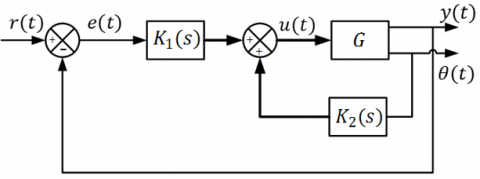
Meanwhile, Figure 3 illustrates the closed-loop block diagram of the liquid slosh control system. Note here, the liquid slosh problem is a single-input-multi-output (SIMO) system. According to Figure 3, the reference being denoted by r(t), the control input being denoted by u(t), and e(t) represents an error. There are two outputs of the system which consists of cart position y(t) and slosh angle θ(t). Meanwhile, the motor-driven liquid tank system is being represented by G. The symbols $K_1(s)$ and $K_2(s)$ represent the FOPID controllers that are responsible to control the cart position and slosh angle, respectively. The FOPID controllers are defined as follows
$K_1(s)=K_{P_1}+K_{I_1} s^{-\lambda_1}+K_{D_1} s^{\mu_1}$, (8)
$K_2(s)=K_{P_2}+K_{I_2} s^{-\lambda_2}+K_{D_2} s^{\mu_2}$, (9)
In Eq. (8) and Eq. (9), $K_{P_1}$ and $K_{P_2}$ are the proportional gains, $K_{I_1}$ and $K_{I_2}$ are the integral gains, $K_{D_1}$ and $K_{D_2}$ are the derivative gains, $\lambda_1$ and $\lambda_2$ are the exponent of integral terms, and $\mu_1$ and $\mu_2$ are the exponent of differential terms.
Figure 3. Closed-loop block diagram of the liquid slosh control system
Table 1. The parameter values for liquid slosh system [27]
|
Parameter |
Value |
Unit |
|
m |
1.32 |
kg |
|
M |
6.0 |
kg |
|
g |
9.81 |
ms-2 |
|
d |
3.0490×10⁻⁴ |
kgm2/s |
|
l |
0.052126 |
m |
As stated in the previous section, this research aims to track the desired reference of cart position and subsequently reduce the liquid slosh level. Thus, the fitness function for the liquid slosh control system as shown in Figure 3 can be presented by
$J\left(\boldsymbol{K}_{\boldsymbol{P}}, \boldsymbol{K}_{\boldsymbol{I}}, \boldsymbol{K}_{\boldsymbol{D}}, \boldsymbol{\lambda}, \boldsymbol{\mu}\right)=w_1 \hat{e}+w_2 \hat{\theta}+w_3 \hat{u}$, (10)
where,
$\hat{e}=\int_0^{t_f}(r(t)-y(t))^2 d t$, (11)
$\hat{\theta}=\int_0^{t_f} \theta(t)^2 d t$, (12)
$\hat{u}=\int_0^{t_f} u(t)^2 d t$. (13)
In (10), $w_1, w_2$ and $w_3$ are the weighting coefficients as per determined by the system's designer. The FOPID controller parameters i.e. $\boldsymbol{K_P}, \boldsymbol{K_I}, \boldsymbol{K}_{\boldsymbol{D}}, \boldsymbol{\lambda}$ and $\boldsymbol{\mu}$ are defined as $\boldsymbol{K_P}:=$ $\left[K_{P_1}, K_{P_2}\right], \boldsymbol{K}_{\boldsymbol{I}}:=\left[K_{I_1}, K_{I_2}\right], \boldsymbol{K}_{\boldsymbol{D}}:=\left[K_{D_1}, K_{D_2}\right], \lambda:=\left[\lambda_1, \lambda_2\right]$, and $\boldsymbol{\mu}:=\left[\mu_1, \mu_2\right]$. Note that, the right side of Eq. (10) is referred to total norm of tracking error $\hat{e}$, total norm of slosh angle $\hat{\theta}$ and total norm of control input $\hat{u}$. Here, the values for weighting coefficients are selected based on undertaken preliminary investigations, such that a well-balanced minimization between tracking error, slosh angle and control input energy is obtained.
Problem 2.1. Find the FOPID controllers parameters $\boldsymbol{K_P}, \boldsymbol{K_I}, \boldsymbol{K_D}, \boldsymbol{\lambda}, \boldsymbol{\mu}$ according to the closed-loop control system in Figure 3, such that the fitness function $J\left(\boldsymbol{K_P}, \boldsymbol{K_I}, \boldsymbol{K}_{\boldsymbol{D}}, \boldsymbol{\lambda}, \boldsymbol{\mu}\right)$ in Eq. (10) is minimized based on measurement input and output data $(u(t), y(t), \theta(t))$.
In this section, the discussion on a data-driven FOPID controller by using the proposed MPA is explained. Firstly, the review on MPA is presented. Then, the procedure in applying the MPA as a tool in tuning the data-driven FOPID controller of the liquid slosh problem is discussed in detail.
3.1 A review on MPA
The marine predators algorithm (MPA) [22], is principally motivated by the foraging strategy of the ocean predators. The main motivation of MPA is to be well-balanced between Brownian walk and Levy walk.
The MPA procedure starts with the randomly distribute the initial solution of each agents within given search space in solving the optimization problem as follows
$\arg \min _{X_i(1), X_i(2) \ldots} f_i\left(X_i(k)\right)$ (14)
for iterations $k=1,2, \ldots, k_{\max }$. In Eq. (14), $X_i$ represents the position vector of agent $i, f_i$ represents the fitness function of agent $i$, and the maximum number of iterations is being denoted by $k_{\max }$. The prey and predators are the agents which can defined by two matrices which are the prey matrix $P$ in Eq. (15) and elite matrix $E$ consisting the best predator in Eq. (16), respectively, as follows
$P=\left[\begin{array}{cccc}X_{1,1} & X_{1,2} & \cdots & X_{1, d} \\ X_{2,1} & X_{2,2} & \cdots & X_{2, d} \\ \vdots & \vdots & \vdots & \vdots \\ X_{n, 1} & X_{n, 2} & \cdots & X_{n, d}\end{array}\right]$, (15)
$E=\left[\begin{array}{cccc}X_{1,1}^{\prime} & X_{1,2}^{\prime} & \cdots & X_{1, d}^{\prime} \\ X_{2,1}^{\prime} & X_{2,2}^{\prime} & \cdots & X_{2, d}^{\prime} \\ \vdots & \vdots & \vdots & \vdots \\ X_{n, 1}^{\prime} & X_{n, 2}^{\prime} & \cdots & X_{n, d}^{\prime}\end{array}\right]$. (16)
In Eq. (15) and Eq. (16), n represents the total number of agents, and the number of dimensions is being denoted by d. In (15), $X_{i, j}$ represents the j-th dimension of i-th prey or agent $X_i$ in Eq. (14). In Eq. (16), the matrix E consists of $X_{i, j}^{\prime}$ which is the j-th element of the best predator vector $X_i^{\prime}$. Then, $X_i^{\prime}$ is replicated n times to form an elite matrix. Next, the prey and predators are updated by using the MPA structure which consists of three main phases, fish aggregating devices’ effect (FADs) and marine memory.
3.1.1 Phase 1
The prey moves faster than the predators in Phase 1 which shows that the prey is the most active agent. Meanwhile, the predators are static, only waiting for the prey. This situation is known as full exploration phase which occurred during the first tierce of the maximum iterations ($k_{\max }$). Thus, the updated equation for the prey in Phase 1 is given as
$P_i=P_i+Q \cdot r_1 \otimes\left[R_B \otimes\left(E_i-R_B \otimes P_i\right)\right], \quad$ if $k<\frac{1}{3} k_{\max }$, (17)
for $i=1,2, \ldots, n$, where $P_i$ is a $i$-th row of matrix $P, E_i$ represent the $i$-th row of matrix $E$, and $R_B$ is a vector of random numbers based on Brownian distribution. Also, the element-wise multiplications is being denoted by the notation $\otimes$. The symbol $Q$ represents the constant number which is set to 0.5 . The random number that is uniformly distributed across the range of $[0,1]$ is represented by symbol $r_1$.
3.1.2 Phase 2
In this phase, both prey and predators are moving at the same pace. The MPA structure in Phase 2 is ready to transit from exploration to exploitation phase by dividing the prey into two groups. The first group of prey perturb its current position towards the exploitation phase by moving in Levy walk. The second group of prey updated its position based on the best predator position towards the exploration phase in which the prey are moving in Brownian walk. This phase occurred after one third of kmax until two third of kmax. Consequently, the first group of prey for i=1,2,…,n⁄2 are updated its location by following equation:
$P_i=P_i+Q . r_1 \otimes\left[R_L \otimes\left(E_i-R_L \otimes P_i\right)\right]$,
if $\frac{1}{3} k_{\max }<k<\frac{2}{3} k_{\max }$, (18)
while, for second group of prey for i=n⁄2, n⁄2+1,…,n, the updated equation is derived as follows:
$P_i=E_i+Q . C F \otimes\left[R_B \otimes\left(R_B \otimes E_i-P_i\right)\right]$,
if $\frac{1}{3} k_{\max }<k<\frac{2}{3} k_{\max }$. (19)
In Eq. (18), the Levy walk is represented by RL which consists of a random number based on Levy distribution. Meanwhile, CF in Eq. (19) represents an adaptive coefficient that controls the predator motion step size which is derived by following equation:
$C F=\left(1-\frac{k}{k_{\max }}\right)^{\left(2 \times \frac{k}{k_{\max }}\right)}$. (20)
3.1.3 Phase 3
The Phase 3 of the MPA structure is performed on the final tierce of the maximum iteration ($k_{\max }$). This phase is also known as the exploitation phase in which the predators follow the Levy walk and move faster than the prey. Hence, the equation to update each prey (i=1, 2,…,n) is given as follows:
$P_i=E_i+Q \cdot C F \otimes\left[R_L \otimes\left(R_L \otimes E_i-P_i\right)\right]$,
if $k>\frac{2}{3} k_{\max }$. (21)
3.1.4 Fish aggregating devices’ effect
Next, the MPA behavior is also considered a fish aggregating devices (FADs) by performing longer vertical jumps into the sea in hopes to locate the location with ample prey. This behavior also can assist the predators to jump out from the local optima region and continue a new search region. Thus, the updated equation for prey by considering FADs effect is given as follows:
$P_i=\left\{\begin{array}{cc}P_i+C F\left[L B+r_1 \otimes(U B-L B)\right] \otimes U, & \text { if } r_2 \leq F A D s, \\ P_i+\left[F A D s\left(1-r_2\right)+r_2\right]\left(P_{r_3}-P_{r_4}\right), & \text { if } r_2>F A D s .\end{array}\right.$ (22)
In Eq. (22), the upper bound is being denoted by UB, the lower bound is being denoted by LB, and FADs is a coefficient that has been set to 0.2. Two random numbers which are $r_1$ and $r_2$ are uniformly produced in range of [0, 1]. Meanwhile, the binary vector which consists of value 0 or 1 is being denoted by symbol U. In particular, U produces array to 1 if $r_2>0.2$. Or else, U generates its array to 0. Additionally, the random indexes of the column of the P matrix are represented by $r_3$ and $r_4$.
3.1.5 Marine memory
The last feature of the MPA structure is marine memory in which the location of high production foraging is saved into memory to avoid local optima solutions. The marine memory can enhance the quality of the produced solutions by comparing the fitness of each solution of the current iteration with the previous iteration. If the current fitness is more fitted, it will replace the previous one. If not, it will maintain the previous solution. This method imitates the predator’s behavior in returning to the most abundant foraging location.
For more detailed explanation on the MPA structure, please refer to the MPA pioneer in the study [22].
3.2 Application of MPA for tuning the data-driven FOPID controller
Here, the procedure in utilizing the MPA as a data-driven tuning tool for the FOPID controller of liquid slosh problem is described in detail. The operational of MPA is focused in minimizing the fitness function in Eq. (10) by tuning ten design parameters of two FOPID controllers of liquid slosh suppression system. The step-by-step procedure for tuning the FOPID controller is stated as follows:
Step 1: Map the fitness function of $f_i=J\left(\boldsymbol{K}_{\boldsymbol{P}}, \boldsymbol{K}_{\boldsymbol{I}}, \boldsymbol{K}_{\boldsymbol{D}}, \boldsymbol{\lambda}, \boldsymbol{\mu}\right)$ and design parameter of $X_{i, j}=\log \left(\boldsymbol{K}_{\boldsymbol{P}}, \boldsymbol{K}_{\boldsymbol{I}}, \boldsymbol{K}_{\boldsymbol{D}}, \boldsymbol{\lambda}, \boldsymbol{\mu}\right)$. Then, determine UB, LB, $k_{\max }, n, d, Q,$ and FADs.
Step 2: Execute the MPA structure in Section 3.
Step 3: Record the optimal design parameters $X_i^{\prime}$ from the best predators in the matrix E as soon as achieving the maximum iteration $k_{\max }$. Then, apply this optimal design parameters to FOPID controllers $K_1(s)$ and $K_2(s)$ in Figure 3.
Remarks 3.1. In this paper, it is highlighted that the tuning of the FOPID controller is based on a data-driven method which solely uses the input and output data with no knowledge towards the model of the plant.
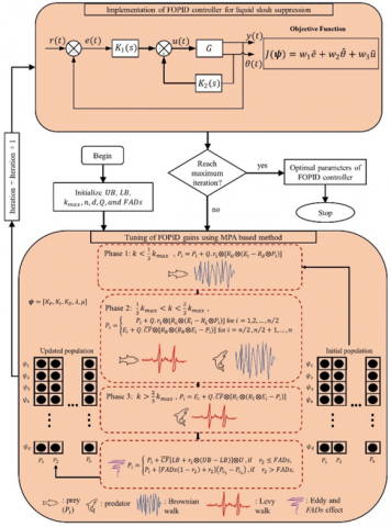
Figure 4 illustrates a detailed flow diagram of the FOPID controller tuning approach using the MPA based method. There are two main blocks: the implementation of the FOPID controller for the AVR system block and the MPA based method block. In the first block, the aim is to obtain the minimal objective function J in Eq. (10). By mapping $f_i$ to $J\left(\boldsymbol{K}_{\boldsymbol{P}}, \boldsymbol{K_I}, \boldsymbol{K}_{\boldsymbol{D}}, \boldsymbol{\lambda}, \boldsymbol{\mu}\right)$, the MPA structure can be executed in the second block to obtain the updated design variable of each prey $X_i$, which is obtained from $P_i$. This updated design variable is then applied to the first block by defining $X_{i, j}=\log \left(\boldsymbol{K}_{\boldsymbol{P}}, \boldsymbol{K}_{\boldsymbol{I}}, \boldsymbol{K}_{\boldsymbol{D}}, \boldsymbol{\lambda}, \boldsymbol{\mu}\right)$. This bidirectional flow between these two main blocks is repeated until reaching the maximum iterations to obtain the optimal design parameter $X_i^{\prime}$.
Figure 4. Flow diagram of MPA implementation for FOPID controller of liquid slosh suppression
Table 2. Optimization settings and simulation settings
|
Optimization settings |
Simulation settings |
|
Upper bound, UB=2.5 |
Simulation time, $t_f$=20s |
|
Lower bound, LB=-2.5 |
|
|
Number of agents, n=20 |
Objective function coefficients, w1=100, w2=100, and w3=5 |
|
Maximum iterations, $k_{\max }$=150 |
|
|
MPA coefficients, Q=0.5 and FADs=0.2 |
|
|
Number of trials=25 |
Table 3. A default coefficient of GWO, SCA, SMA, and MVO
|
Algorithm |
Coefficients |
|
GWO |
$a=2 *\left(1-\left(\frac{k}{k_{\max }}\right)\right)$ |
|
SCA |
$r_1=2 *\left(1-\left(\frac{k}{k_{\max }}\right)\right)$ |
|
SMA |
$\begin{gathered}a=\operatorname{arctanh}\left(-\left(\frac{k}{k_{\max }}\right)+1\right) \\ z=0.03\end{gathered}$ |
|
MVO |
$W E P_{\min }=0.2, W E P_{\max }=1, p=6$ |
In this section, the performance investigation of the liquid slosh control system by using a FOPID controller based on the MPA is presented. Here, the effectiveness of the proposed MPA-FOPID controller in solving the liquid slosh problem is compared with GWO-FOPID [28], SCA-FOPID [29], SMA-FOPID [30], MVO-FOPID [31] and SPSA-PID controller [27]. In this study, the main performance criteria are based on the convergence curve of the average fitness function. Besides that, the statistical results out of 25 trials for the fitness function J, total norm of tracking error and slosh angle, and total norm of control input are scrutinized in terms of average, worst, best and standard deviation (std.). Next, to scrutinize the non-parametric statistical test, the Wilcoxon’s rank test is conducted to differentiate between the MPA based method and other metaheuristic optimization based methods.
In this study, the simulation platform is based on MATLAB/Simulink R2020a. The simulation exercises are performed utilizing a personal computer with an operating system of Microsoft Windows 10. The processor is powered by Intel Core i7-6700 Processor (3.41GHz) with the RAM of 8GB. According to Eq. (8) and Eq. (9), there are 5 controller parameters for each FOPID controller. Therefore, there are 10 controller parameters of the FOPID controller to be tuned by MPA. The weighting coefficients were set to w1=100, w2=100, and w3=5, which is the same as the setting in the study [27]. Here, the simulation time is set as tf=20s. In this study, the reference of the cart position is formulated as follows
$r(t)=\left\{\begin{array}{cc}0, & 0 \leq t \leq 0.5, \\ 0.5, & 0.5<t \leq 20.\end{array}\right.$ (23)
Next, the upper bound UB is set to 2.5 and lower bound LB is set to -2.5 for each FOPID controller parameters. Meanwhile, there are 20 number of agents n and the maximum number of iterations $k_{\max}$ is set to 150. Thus, there are 3000 number of function evaluations (NFE) is performed for each algorithm. There are 25 independent trials conducted to evaluate the efficacy of each algorithm in examining the randomization effect. Table 2 summarizes the optimization settings and simulation settings for this study. Meanwhile, Table 3 tabulates the coefficients for other compared algorithms which are GWO, SCA, SMA and MVO based methods.
Remarks 4.1. It is noted here, the same upper bounds, lower bounds, number of agents, and maximum number of iterations are set for each compared algorithm for a fairly comparison assessment.
The first performance criteria considered in this study is a convergence curve of the average fitness function produced by all algorithms running for 25 independent trials. Figure 5 illustrates the average fitness function convergence curves for MPA, GWO, SCA, SMA and MVO based methods with the magnified plot at the end of iteration to highlight the most minimized fitness function. From the magnified version of Figure 5, we can see that the MPA based method has demonstrated excellence performance by producing the most minimum value of fitness function at the end of iteration as compared to other algorithms. Additionally, Table 4 scrutinizes the investigation of the statistical results for MPA-FOPID, GWO-FOPID, SCA-FOPID, SMA-FOPID and MVO-FOPID controllers, as well as previously published SPSA-PID controller in terms of fitness function J, total norm of tracking error and slosh angle, and total norm of control input. Note here, for SPSA-PID controller, the statistical results are taken directly from their paper [27]. As can be seen from Table 4, the MPA-FOPID has generated superior results for average, best, worst and standard deviation of fitness function as highlighted in bold. Meanwhile, for total norm of tracking error and slosh angle, the MPA-FOPID has dominated for the majority of the assessed domains as indicated in bold font except for best domain which is won by the SCA-FOPID controller. Further statistical results revealed the total norm of control input generated by MPA-FOPID is better for average, worst and standard deviation domains except for best domain which is dominated by SCA-FOPID. Interestingly, these statistical results show that the MPA-FOPID has a consistency in producing a superior result for each trial despite facing a randomization effect. The consistency of the MPA-FOPID can be proved by the graphical box plot of the fitness function as shown in Figure 6. It can be seen from the box plot that the proposed MPA-FOPID produced the smallest interquartile range which indicated the high consistency level and high precision.
Merely analyzing the statistical results is insufficient to distinguish which algorithm is better in minimizing the fitness function since the statistical results do not compare for each trial. For 25 independent trials, there is a possibility the losing algorithm can produce a better result compared to the one who won the overall statistical results. Thus, a non-parametric statistical test is conducted to evaluate the statistical difference in order to decide whether the better algorithm is significant or not. In this study, the Wilcoxon’s rank test is used to differentiate two algorithms by undergoing the statistical test and comparing the p-value. Wilcoxon’s rank test stated that the p-value should be less than 0.05 to show that the better algorithm is significantly different to other algorithms. Table 5 presents the results obtained from the Wilcoxon’s rank test between the MPA based method and other compared based methods. As shown in Table 5, all p-values reported are less than 0.05 which signified the superior significant difference between MPA based method and other metaheuristic optimization based methods. Taken together, these results show that the proposed MPA based method can provide a good balancing between exploration and exploitation phases as well as avoiding capability from the local optima in comparison with other metaheuristic optimization based methods.
The next performance criteria was concerned with the time response of the cart position, slosh angle and control input energy. For fair comparison, all algorithms take the FOPID controller parameters obtained from the best fitness function out of 25 trials. Table 6 tabulates the best FOPID controller parameters obtained by MPA, GWO, SCA, SMA and MVO. The cart position responses obtained by all metaheuristic optimization based methods are presented in Figure 7. Based on the responses, all algorithms achieve approximately the same settling time which is 6.5s. The main difference is the percentage overshoot where the SCA-FOPID produces the highest percentage overshoot with 6.08% while the proposed MPA-FOPID scores the second lowest percentage overshoot which is 4.38%. Meanwhile, for the slosh angle responses as shown in Figure 8, all algorithms also produce approximately the same response with the proposed MPA having very competitive results with score the fourth lowest slosh angle which is 0.063 radian compared to the lowest slosh angle by SCA with score 0.062 radian. Lastly, the control input responses are shown in Figure 9. The highest control input energy is produced by MVO with score 2.32N, while the proposed MPA has produces the third lowest control input energy which is 2.23N. Overall, we can say that the MPA-FOPID controller has a good time responses by producing the competitive results for cart position, slosh angle and control input energy. Thus, it is verified that the proposed MPA based method is a better data-driven tuning tool for the FOPID controller in minimizing the fitness function of the liquid slosh suppression system as compared to other metaheuristic optimization based methods.
Figure 5. Convergence curves of the average fitness function produced by different algorithms
Table 4. The statistical results for all controllers
|
Controller |
MPA-FOPID |
GWO-FOPID [28] |
SCA-FOPID [29] |
SMA-FOPID [30] |
MVO-FOPID [31] |
SPSA-PID [27] |
|
|
J |
Average |
41.1170 |
44.4082 |
47.4232 |
42.1543 |
48.6400 |
41.8345 |
|
Best |
41.1050 |
41.1160 |
41.1732 |
41.1054 |
41.1228 |
41.1081 |
|
|
Worst |
41.1470 |
55.2452 |
57.0222 |
55.9529 |
56.1046 |
42.7285 |
|
|
Std |
0.0099 |
5.2203 |
5.9721 |
3.1523 |
6.0648 |
0.5136 |
|
|
Total norm of tracking error and slosh angle |
Average |
0.3095 |
0.3349 |
0.3681 |
0.3189 |
0.3702 |
0.3146 |
|
Best |
0.3087 |
0.3092 |
0.2901 |
0.3089 |
0.3090 |
0.3040 |
|
|
Worst |
0.3100 |
0.4122 |
0.4573 |
0.4311 |
0.4330 |
0.3297 |
|
|
Std |
3.01E-04 |
0.0395 |
0.0549 |
0.0262 |
0.0454 |
0.0072 |
|
|
Total norm of input |
Average |
2.0328 |
2.1832 |
2.1122 |
2.0512 |
2.3168 |
2.1693 |
|
Best |
2.0238 |
2.0069 |
1.0439 |
1.9469 |
1.6050 |
1.9103 |
|
|
Worst |
2.0513 |
2.8028 |
3.1815 |
2.5625 |
2.7513 |
3.2530 |
|
|
Std |
0.0068 |
0.2593 |
0.5805 |
0.1141 |
0.4092 |
0.2431 |
|
Table 5. p-value from Wilcoxon’s rank test
|
MPA Versus |
||||
|
Algorithm |
GWO [28] |
SCA [29] |
SMA [30] |
MVO [31] |
|
p-value |
8.2737E-09 |
1.4144E-09 |
2.7759E-05 |
5.2076E-09 |
Table 6. The FOPID controller parameters obtained from the best fitness function
|
FOPID controller parameters |
MPA |
GWO [28] |
SCA [29] |
SMA [30] |
MVO [31] |
|||||
|
$X_i^{\prime}$ |
$10^{X_i^{\prime}}$ |
$X_i^{\prime}$ |
$10^{X_i^{\prime}}$ |
$X_i^{\prime}$ |
$10^{X_i^{\prime}}$ |
$X_i^{\prime}$ |
$10^{X_i^{\prime}}$ |
$X_i^{\prime}$ |
$10^{X_i^{\prime}}$ |
|
|
$K_{P_1}$ |
0.5064 |
3.2091 |
-0.0308 |
0.9316 |
0.3555 |
2.2673 |
0.5342 |
3.4215 |
-2.2980 |
0.0050 |
|
$K_{I_1}$ |
-2.4969 |
0.0032 |
-0.0176 |
0.9602 |
0.1795 |
1.5119 |
0.6269 |
4.2351 |
-2.0642 |
0.0086 |
|
$K_{D_1}$ |
0.1010 |
1.2618 |
0.4210 |
2.6361 |
-0.0416 |
0.9086 |
-0.0094 |
0.9787 |
0.6445 |
4.4104 |
|
$\lambda_1$ |
-0.8045 |
0.1569 |
-0.8617 |
0.1375 |
-0.8165 |
0.1526 |
2.3773 |
238.4168 |
-2.2064 |
0.0062 |
|
$\mu_1$ |
-2.2449 |
0.0057 |
-1.6196 |
0.0240 |
-1.0417 |
0.0908 |
-1.3550 |
0.0442 |
-1.9275 |
0.0118 |
|
$K_{P_2}$ |
-0.0789 |
0.8337 |
0.0728 |
1.1824 |
-2.4447 |
0.0036 |
-0.2233 |
0.5980 |
-0.3345 |
0.4630 |
|
$K_{I_2}$ |
1.8565 |
71.8623 |
1.8641 |
73.1349 |
1.8832 |
76.4183 |
1.8448 |
69.9496 |
1.8481 |
70.4808 |
|
$K_{D_2}$ |
-0.2960 |
0.5058 |
-0.3439 |
0.4530 |
-0.1451 |
0.7160 |
-0.2899 |
0.5130 |
-0.1320 |
0.7378 |
|
$\lambda_2$ |
0.0002 |
1.004 |
0.0093 |
1.0217 |
0.0031 |
1.0072 |
-0.0005 |
0.9988 |
-0.0014 |
0.9968 |
|
$\mu_2$ |
0.0156 |
1.0365 |
0.0278 |
1.0661 |
-0.0066 |
0.9848 |
0.0133 |
1.0312 |
-0.0251 |
0.9438 |
Figure 6. Box plot of the fitness function
Figure 7. Cart position responses by different algorithms
Figure 8. Slosh angle responses by different algorithms
Figure 9. Control input responses by different algorithms
In this paper, we have proposed a data-driven tuning tool for the FOPID controller of liquid slosh suppression system based on marine predators algorithm (MPA). From the obtained results, the MPA-FOPID controller has outperformed other recent metaheuristic optimization tuned FOPID controller as well as SPSA-PID controller in terms of average convergence curve, statistical results of fitness function, total norm of tracking error, total norm of slosh angle and total norm of control input. Additionally, the MPA based method is significantly different with other metaheuristic optimization algorithms as has been verified by the Wilcoxon’s rank test. Hence, it has been justified that the proposed MPA based method is a good choice in tuning the FOPID controller for solving the liquid slosh problem. Lastly, due to feasibility and applicability of the algorithm, it can be a good candidate as a data-driven tuning tool for other controllers of practical applications in improving the system performance.
This work is supported by the Malaysian Ministry of Higher Education (Grant numbers: FRGS/1/2021/TK0/UMP/02/5) (University reference RDU210106). Also, thanks to Universiti Malaysia Pahang and Universiti Teknikal Malaysia Melaka for supporting in terms of facilities in completing this current paper.
[1] Troll, C., Majschak, J.P. (2020). Modeling transient liquid slosh behavior at variable operating speeds induced by intermittent motions in packaging machines. Applied Sciences, 10(5): 1859. https://doi.org/10.3390/app10051859
[2] Troll, C., Tietze, S., Majschak, J.P. (2020). Controlling liquid slosh by applying optimal operating-speed-dependent motion profiles. Robotics, 9(1): 18. https://doi.org/10.3390/robotics9010018
[3] Saltari, F., Traini, A., Gambioli, F., Mastroddi, F. (2021). A linearized reduced-order model approach for sloshing to be used for aerospace design. Aerospace Science and Technology, 108: 106369. https://doi.org/10.1016/j.ast.2020.106369
[4] Liu, L., Feng, D., Wang, X., Zhang, Z., Yu, J., Chen, M. (2022). Numerical study on the effect of sloshing on ship parametric roll. Ocean Engineering, 247: 110612. https://doi.org/10.1016/j.oceaneng.2022.110612
[5] Zheng, J., Li, G., Teng, X., Qiu, Z. (2020). Analysis and research of molten copper sloshing in mould of anode based on VOF method. In IOP Conference Series: Materials Science and Engineering. IOP Publishing, 711(1): 012031. https://doi.org/10.1088/1757-899X/711/1/012031
[6] Jalili, M.M., Motavasselolhagh, M., Fatehi, R., Sefid, M. (2022). Investigation of sloshing effects on lateral stability of tank vehicles during turning maneuver. Mechanics Based Design of Structures and Machines, 50(9): 3180-3205. https://doi.org/10.1080/15397734.2020.1800490
[7] Tsao, W.H., Huang, L.H., Hwang, W.S. (2021). An equivalent mechanical model with nonlinear damping for sloshing rectangular tank with porous media. Ocean Engineering, 242: 110145. https://doi.org/10.1016/j.oceaneng.2021.110145
[8] Yu, L., Xue, M.A., Jiang, Z. (2020). Experimental investigation of parametric sloshing in a tank with vertical baffles. Ocean Engineering, 213: 107783. https://doi.org/10.1016/j.oceaneng.2020.107783
[9] Khorshid, E., Al-Fadhli, A. (2021). Optimal command shaping design for a liquid slosh suppression in overhead crane systems. Journal of Dynamic Systems, Measurement, and Control, 143(2). https://doi.org/10.1115/1.4048357
[10] Alshaya, A., Alshayji, A. (2022). Robust multi-steps input command for liquid sloshing control. Journal of Vibration and Control, 28(19-20): 2607-2624. https://doi.org/10.1177/10775463211017721
[11] Zang, Q., Huang, J., Liang, Z. (2014). Slosh suppression for infinite modes in a moving liquid container. IEEE/ASME Transactions on Mechatronics, 20(1): 217-225. https://doi.org/10.1109/TMECH.2014.2311888
[12] Tumari, M.Z.M., Subki, A.S.R.A., Aras, M.S.M., Ahmad, M.A., Suid, M.H. (2019). H-infinity controller with graphical LMI region profile for liquid slosh suppression. TELKOMNIKA (Telecommunication Computing Electronics and Control), 17(5): 2636-2642. http://doi.org/10.12928/telkomnika.v17i5.11252
[13] Al-Mashhadani, M.A. (2020). Modeling and adaptive robust wavelet control for a liquid container system under slosh and uncertainty. Measurement and Control, 53(9-10): 1643-1653. https://doi.org/10.1177/0020294020952487
[14] Dou, L., Du, M., Zhang, X., Du, H., Liu, W. (2019). Fuzzy disturbance observer-based sliding mode control for liquid-filled spacecraft with flexible structure under control saturation. IEEE Access, 7: 149810-149819. https://doi.org/10.1109/ACCESS.2019.2946961
[15] Piga, D., Formentin, S., Bemporad, A. (2017). Direct data-driven control of constrained systems. IEEE Transactions on Control Systems Technology, 26(4): 1422-1429. https://doi.org/10.1109/TCST.2017.2702118
[16] Borase, R.P., Maghade, D.K., Sondkar, S.Y., Pawar, S.N. (2021). A review of PID control, tuning methods and applications. International Journal of Dynamics and Control, 9: 818-827. https://doi.org/10.1007/s40435-020-00665-4
[17] Podlubny, I. (1999). Fractional-order systems and PI/sup/spl lambda//D/sup/spl mu//-controllers. IEEE Transactions on Automatic Control, 44(1): 208-214. https://doi.org/10.1109/9.739144
[18] Jamil, A.A., Tu, W.F., Ali, S.W., Terriche, Y., Guerrero, J.M. (2022). Fractional-order PID controllers for temperature control: A review. Energies, 15(10): 3800. https://doi.org/10.3390/en15103800
[19] Mok, R., Ahmad, M.A. (2022). Fast and optimal tuning of fractional order PID controller for AVR system based on memorizable-smoothed functional algorithm. Engineering Science and Technology, an International Journal, 35: 101264. https://doi.org/10.1016/j.jestch.2022.101264
[20] Acharya, D.S., Sarkar, B., Bharti, D. (2020). A fractional order particle swarm optimization for tuning fractional order PID controller for magnetic levitation plant. In 2020 First IEEE International Conference on Measurement, Instrumentation, Control and Automation (ICMICA), pp. 1-6. https://doi.org/10.1109/ICMICA48462.2020.9242792
[21] Vanchinathan, K., Selvaganesan, N. (2021). Adaptive fractional order PID controller tuning for brushless DC motor using artificial bee colony algorithm. Results in Control and Optimization, 4: 100032. https://doi.org/10.1016/j.rico.2021.100032
[22] Faramarzi, A., Heidarinejad, M., Mirjalili, S., Gandomi, A.H. (2020). Marine predators algorithm: A nature-inspired metaheuristic. Expert Systems with Applications, 152: 113377. https://doi.org/10.1016/j.eswa.2020.113377
[23] Tumari, M.Z.M., Ahmad, M.A., Suid, M.H., Ghazali, M.R. (2022). Data-driven control based on marine predators algorithm for optimal tuning of the wind plant. In 2022 IEEE International Conference on Power and Energy (PECon), pp. 203-208. https://doi.org/10.1109/PECon54459.2022.9988895
[24] Yakout, A.H., Sabry, W., Abdelaziz, A.Y., Hasanien, H.M., AboRas, K.M., Kotb, H. (2022). Enhancement of frequency stability of power systems integrated with wind energy using marine predator algorithm based pida controlled statcom. Alexandria Engineering Journal, 61(8): 5851-5867. https://doi.org/10.1016/j.aej.2021.11.011
[25] Yakout, A., Sabry, W., Hasanien, H.M. (2021). Enhancing rotor angle stability of power systems using marine predator algorithm based cascaded PID control. Ain Shams Engineering Journal, 12(2): 1849-1857. https://doi.org/10.1016/j.asej.2020.10.018
[26] Padhy, S., Sahu, P.R., Khadanga, R.K., Prusty, B.R., Panda, S. (2021). MPA-tuned fractional order PID controller for frequency control of interconnected smart grid power system. In 2021 Innovations in Power and Advanced Computing Technologies (i-PACT). IEEE, pp. 1-5. https://doi.org/10.1109/i-PACT52855.2021.9696651
[27] Mustapha, N.M.Z.A., Mohd Tumari, M.Z., Suid, M.H., Raja Ismail, R.M.T., Ahmad, M.A. (2019). Data-driven PID tuning for liquid slosh-free motion using memory-based spsa algorithm. In Proceedings of the 10th National Technical Seminar on Underwater System Technology 2018: NUSYS'18. Springer Singapore, pp. 197-210. https://doi.org/10.1007/978-981-13-3708-6_17
[28] Mirjalili, S., Aljarah, I., Mafarja, M., Heidari, A.A., Faris, H. (2020). Grey wolf optimizer: theory, literature review, and application in computational fluid dynamics problems. Nature-Inspired Optimizers: Theories, Literature Reviews and Applications, 87-105. https://doi.org/10.1007/978-3-030-12127-3_6
[29] Gabis, A.B., Meraihi, Y., Mirjalili, S., Ramdane-Cherif, A. (2021). A comprehensive survey of sine cosine algorithm: Variants and applications. Artificial Intelligence Review, 54(7): 5469-5540. https://doi.org/10.1007/s10462-021-10026-y
[30] Li, S., Chen, H., Wang, M., Heidari, A.A., Mirjalili, S. (2020). Slime mould algorithm: A new method for stochastic optimization. Future Generation Computer Systems, 111: 300-323. https://doi.org/10.1016/j.future.2020.03.055
[31] Aljarah, I., Mafarja, M., Heidari, A.A., Faris, H., Mirjalili, S. (2020). Multi-verse optimizer: Theory, literature review, and application in data clustering. Nature-Inspired Optimizers: Theories, Literature Reviews and Applications, 123-141. https://doi.org/10.1007/978-3-030-12127-3_8