Yahya Dogan![]()
(This article is part of the Special Issue Advances of Machine Learning and Deep Learning)
© 2023 IIETA. This article is published by IIETA and is licensed under the CC BY 4.0 license (http://creativecommons.org/licenses/by/4.0/).
OPEN ACCESS
Global Pooling (GP) is one of the important layers in deep neural networks. GP significantly reduces the number of model parameters by summarizing the feature maps and enables a reduction in the computational cost of training. The most commonly used GP methods are global max pooling (GMP) and global average pooling (GAP). The GMP method produces successful results in experimental studies but has a tendency to overfit training data and may not generalize well to test data. On the other hand, the GAP method takes into account all activations in the pooling region, which reduces the effect of high activation areas and causes a decrease in model performance. In this study, a GP method called global average of top-k max pooling (GAMP) is proposed, which returns the average of the highest k activations in the feature map and allows for mixing the two methods mentioned. The proposed method is compared quantitatively with other GP methods using different models, i.e., Custom and VGG16-based and different datasets, i.e., CIFAR10 and CIFAR100. The experimental results show that the proposed GAMP method provides better image classification accuracy than the other GP methods. When the Custom model is used, the proposed GAMP method provides a classification accuracy of 1.29% higher on the CIFAR10 dataset and 1.72% higher on the CIFAR100 dataset compared to the method with the closest performance.
global pooling, convolutional neural network, deep learning, image classification, transfer learning
Deep neural networks (DNNs) are a type of artificial neural network consisting of multiple layers and interconnected artificial neurons. DNNs are inspired by the structure and function of the human brain; it learns from examples to recognize patterns and relationships in data. The importance of DNNs stems from their ability to learn complex representations of data and make accurate predictions. Some of the key benefits of DNNs are: (1) Improved accuracy; DNNs have achieved state-of-the-art results in various tasks, outperforming traditional machine learning methods in many problems, (2) Hierarchical learning; DNNs can learn hierarchical representations of data that capture more and more complex features as the data forwards from the input layer to the deeper layers of the network, (3) Automated feature extraction; DNNs can automatically learn useful features from raw data without the need for manual feature selection, (4) Handling of large-scale and complex data; DNNs can handle large-scale and complex data, making them suitable for tasks, e.g. image and speech recognition [1, 2], natural language processing [3], and machine translation [4], etc., and (5) Transfer learning: DNNs can be used as a pre-trained model for other tasks, reducing the amount of data and computational resources required to train a model from scratch. The depth and capacity of DNNs increase depending on the size and complexity of the problem to be solved.
Convolutional neural networks (CNNs) are a special type of DNN that have recently provided state-of-the-art results in many problems in computer vision [4, 5]. A standard CNN consists of convolution, activation function, local pooling, flatten, and fully connected (FC) layers at the top. The convolution layers are used to detect features in the image. These layers contain various kernels that combine each pixel in the image with the pixels around it to detect features in the image. Initially, these kernels, which are randomly generated, are slid over the input image or the feature maps from the previous layer to create new feature maps for the next layer. This process determines the regions in the image where the features are located and allows to use of these features in later layers. The activation function determines the effect of weight values that regulate the operation of artificial neurons. It is commonly referred to as a squashing function and determines whether a neuron is activated or not. Activation functions are generally non-linear, which gives the model the ability to be non-linear. The local pooling layer reduces the size of the input images or feature maps, which reduces the calculations required during training and increases the training speed. It also makes the model more robust to small changes, e.g., minor shifts in the image, which enables the model to have better generalization ability on images. However, the local pooling operation causes information loss, as it attempts to represent the pixels within a defined kernel with a single value. Therefore, small kernel sizes, e.g., 2×2 or 3×3, are often used to keep the information loss low. The flatten layer converts the input tensor into a one- dimensional vector by flattening it. This layer is usually used as a preprocessing step before the data is passed to an FC layer. The main purpose of the flatten layer is to transform a multi-dimensional input tensor into a one-dimensional vector. This is important because FC layers expect a one-dimensional input; therefore, the input must be reshaped in order to be passed to the FC layer. For example, an input tensor with shape (batch size, height, width, channels) is transformed into a one-dimensional tensor with shape (batch size, height * width * channels) using a flatten layer. An FC layer, also known as a dense layer, is a type of layer that connects input data to output data. This consists of a set of weights and biases applied to the input data and produces the output tensor. The main purpose of this layer is to learn high-level features from the input data. It does this by applying weights and biases that transform the input data into a meaningful and informative new representation. Since this layer connects all the neurons in the input layer and the output layer, the number of model parameters increases significantly depending on the number of neurons in the input layer.
The feature maps in the last layer of the model are flattened with the flatten layer, and each neuron is connected to the output layer with its FC layer. The number of model parameters increases significantly depending on the resolution of the feature maps in the last layer of the model. Recently, Lin et al. [6] proposed to directly output the confidence of the feature maps using the GP methods rather than connecting the feature maps from the last convolutional layer to the output layer with FC layers. This provides a more meaningful and interpretable method that challenges the fit between feature maps and categories/classes instead of the black-box FCs in CNNs. In addition, FC layers tend to be prone to overfitting; therefore, regularization techniques, e.g., dropout [7], are often used between FC layers. On the other hand, GP naturally has a regularizer that prevents overfitting. Recently, the state-of-the-art models proposed for computer vision problems have been observed to use GMP or GAP layers in the last layer.
Global pooling methods convert the feature map obtained from the last layer of the model into a single scalar value regardless of resolution. This reduces the complexity and computational requirements of the model by minimizing the spatial dimensions of the feature maps. GMP outputs the highest activation in the pooling region, while GAP outputs the average of all activation values in the pooling region. Experimental studies conducted by researchers have reported that the max-pooling layer provides excellent empirical results [7, 8], but is overfitting to training data and does not guarantee generalization on test data. Average pooling, on the other hand, considers all elements in the pooling region, which indicates that low activation areas reduce the effect of high activation areas [9-11]. In this study, a method called Global Average of top-k Max-pooling (GAMP) is proposed, inspired by the top- k max-pooling method proposed in the field of word embedding [12]. Word embedding is a technique used in natural language processing to represent words as numerical vectors in high dimensions. These vectors capture the context and meaning of the words in the text and are used in machine-learning models. In the top-k max pooling technique proposed in the field of natural language processing, the highest-valued words in the pooling region are selected and the other elements are set to zero. It is reported that this provides to preserve the most important information in the pooling region and improve the performance of the model [12]. In the proposed GAMP method, the average of the k neurons with the highest activation is produced as the output. In other words, instead of producing k outputs for each feature map, a single value is produced. The motivation behind the proposed GAMP method is to increase the performance of DNNs by finding a compromise between GP methods, i.e., GAP and GMP, and reducing the limitations present in these methods.
The main contributions of this study can be summarized as follows:
• A new GP method is proposed by considering the disadvantages of current methods. The proposed method increases the generalization ability of the model by preserving high activation. This provides an improvement in classification performance on the test dataset.
• The proposed method was compared to other methods in the same category using both a Custom model and a popular CNN model, i.e., VGG16-based, and the success of the proposed method was demonstrated experimentally.
• A similar approach proposed for word embedding studies was adapted to the classification problem and compared. In this study, it was shown that the proposed GAMP method provides better results.
• Experimental studies were conducted and recommendations have been made for different models, i.e., Custom and VGG16-based, different datasets, e.g., CIFAR10 and CIFAR100, and different k values ranging from 0 to 10 for the reference of researchers.
The rest of the article is organized as follows. A brief summary of related previous studies is given in Section 2. The proposed method and materials used are discussed in detail in Section 3. Method comparison results are given in Section 4. The article ends with future directions.
The pooling layer enables down sampling on the feature maps obtained from the previous layer, reducing the input size of the feature maps significantly and producing meaningful compact outputs. There are two main advantages of using a pooling layer in deep models: (1) It significantly reduces computation cost by reducing the spatial resolution of the feature maps, and (2) It extracts only useful information from the feature maps, i.e., it discards unnecessary details and performs global feature selection for the pooling area, controlling overfitting and increasing test performance. Selecting an ideal pooling layer can increase the success of deep CNN models in tasks, e.g., classification, perception, and segmentation. In CNN models, two types of pooling layers are used: local and global. Local pooling is placed between convolution layers and reduces the resolution of feature maps. In this method, a predetermined kernel (generally of low dimensions such as 2×2, 3×3, etc.) is slid over the feature maps and a feature selection is made for the relevant pooling region.
There are many approaches suggested in this context since the local pooling technique has been used since the first CNNs were proposed. These studies can be classified into four categories: value, probability, rank, and transformed. In the value-based pooling method, an activation is selected based on predetermined criteria, e.g., the highest or most important, from among the activations in the relevant pooling region. There are many approaches suggested based on activation selection: Max-Pooling [13], Average pooling [5], Mixed pooling [14], Detail preserving pooling [15], LEAP pooling [16], Spatial pyramid pooling [17], Kernel pooling [18], and Dynamic correlation pooling [19]. The max-pooling [13] selects the largest activation from the pooling region and eliminates non-maximum values, resulting in reduced computation in higher layers. The average pooling [5] method calculates the average of all activations within a pooling region. Mixed pooling [14] uses a tunable parameter to select either max or average pooling during the training of CNNs, effectively mitigating over-fitting in deep CNNs. The detail preserving Pooling [15], inspired by the human visual system’s focus on local spatial details, enhances spatial changes and provides an adaptive pooling approach that preserves significant structural details through the utilization of an inverse bilateral filter. In the related method, a learnable parameter is used that regulates the reduction of the feature map. The LEAP pooling [16] uses a shared linear filter on each map to process each input feature channel individually and combines the features within the pooling region. This helps to minimize both the number of parameters and the training error. The spatial pyramid pooling [17] generates a fixed-length output that remains consistent regardless of the input size. This eliminates the need for cropping the input image to reach the desired size and reduces the loss of information resulting from cropping, thereby improving the model’s performance. The kernel pooling [19] enables the capturing of high-level and non-linear attribute interactions through compact attribute matching. The proposed method is fully differentiable, making it possible to learn the composition of the kernel in conjunction with CNNs through backpropagation using the data. Dynamic correlation pooling [18] provides a method based on the Mahalanobis distance between adjacent pixels in an image. In this method, one of max, average, or mixed pooling is dynamically selected based on the correlation between the Mahalanobis distance and a specified threshold distance.
In probability-based pooling methods, a trade-off is often made between max pooling and average pooling, which are commonly used in CNNs. This approach combines the two methods and provides a hybrid approach, which allows for a more balanced representation of the pooling area while still preserving the most important information. To benefit from the advantages of both methods and avoid the disadvantages, various methods have been proposed, e.g., Lp pooling [20], Stochastic pooling [9], Max pooling dropout [21], Sparsity-based stochastic pooling [22], and Hybrid pooling method [23], based on the mixing mechanism used. In Lp pooling [20], the type of pooling is determined by the probability value P. When P=1, it represents a straightforward Gaussian mean, and when P=∞, it represents max-pooling. The objective of this related method is to give more significance to strong features and suppress weak ones. Stochastic pooling [9] is a method that replaces deterministic pooling with a stochastic procedure. The activations in the pooling region are normalized to determine probabilities, and then a random activation is selected according to a multinomial distribution, allowing for non-maximum activations in feature maps. Unlike max and average pooling, the stochastic pooling method is not negatively impacted by regularization techniques like dropout and can be combined with other forms of regularization. The max pooling dropout [21] investigated the effect of the dropout technique on pooling layers in CNN architectures. It has been stated experimentally that the related method performs better than the maximum and scaled maximum probability. The sparsity-based stochastic pooling [22] utilizes the sparsity of activations and a control function to obtain a feature representation that balances the pros and cons of max and average pooling. Additionally, the method incorporates weighted random sampling to retain the benefits of stochastic pooling. Hybrid pooling [23] combines max and average pooling methods. It calculates both max and average pooling values for the same region and applies a determined probability of these values. Experiment results indicate that using a 0.75: 0.25 ratio for max and average pooling values is more successful.
In the rank-based pooling method, the activations in the pooling region are grouped according to a predetermined ranking method. Later, the activation within each group is multiplied by a weight value to produce the output. This method allows for the dataset to be ranked based on the values of the activations. The relevant weight values can generally be trained and updated using the back-propagation algorithm [24-26]. The rank-based pooling method is less commonly used than other pooling methods, but it can be useful in certain applications and is preferred in tasks where the activations need to be ranked according to their values. These methods are grouped into three categories based on their weight assignment techniques: RAP (Rank-Based Average Pooling), RWP (Rank-Based Weighted Pooling), and RSP (Rank-Based Stochastic Pooling). In the RAP approach, the top t (e.g., 4) activations in the pooling region are considered, while the rest are discarded. The average of these selected activations is then calculated for the relevant pooling region. RAP strikes a balance between max pooling and average pooling, and offers improved discrimination compared to these methods. The RWP approach recognizes the fact that not all regions in an image have equal importance. It calculates a weighted average by multiplying each activation in the pooling region with an appropriate coefficient. In RWP, weights are assigned rationally based on the magnitude of the activations. The activation with the highest magnitude receives the highest weight, and conversely, the lowest activation gets the smallest weight. The RSP method replaces conventional pooling operations with a stochastic process, where the probabilities of the activations are selected from a multinomial distribution. In RSP, the calculation of probabilities is based on the order of activations, not their values, unlike value-based stochastic pooling. The significant advantage of this approach is the high degree of randomness in activation selection. However, its drawback is that it has a large number of learnable parameters, leading to increased memory usage and decreased processing speed.
In the transformed domain-based pooling method, a transformation is applied using domains such as time, space, frequency, and wavelet domain, to reduce the variability in feature maps. In these methods, the frequency domain is generally taken as a reference and high frequencies in the pooling region are captured [27-29]. When local pooling techniques are generally evaluated, the pooling region has low dimensions, such as 2×2 or 3×3, so the information loss is relatively low. It even allows the model to avoid overfitting and increases the model’s generalization ability. Pooling layers reduce the number of parameters and limit the model’s ability to memorize training data, which provides prevent overfitting. However, it is seen that state-of-the-art local pooling methods developed in this context only slightly increase model performance, e.g., <1.
GP methods are used at the end of CNNs and produce a single value for each feature map [30]. These methods are used to minimize the spatial dimensions of the output of the CNN and simplify the final classification. In general, the flatten layer is used in the last layer of CNN models to convert values in the feature map into neurons, and these neurons are then connected to the output layer through FC layers. In the GP method, the number of model parameters is greatly reduced as each feature map is converted to a single value, and therefore the computational cost is reduced. In the literature, the GMP and GAP [6] methods are widely used. In the GMP method, the highest activation value in the feature map in the final layer is produced as the output. However, as previously mentioned, this technique suffers from a lack of generalization ability. In the GAP method, the output is produced by taking the average of all activations in the feature map. This method can also suppress high activations and negatively affect the performance of the model. In addition, this problem deepens as the resolution of the feature map increases in GP techniques. In local pooling techniques, the resolution of the pooling region is small, e.g., 2×2 or 3×3, while in global pooling techniques the resolution of the pooling region is large, e.g., 7×7, 14×14, or 28×28. Taking the highest or average value in this large area can significantly affect the performance of the model.
In this section, existing GP methods, the proposed GAMP method, public datasets used in experimental studies, CNN models created for comparison of methods, and training details are discussed. In the scope of the study, GP methods are compared based on a classification problem.
3.1 Global pooling methods
In classification problems, the feature maps obtained after the last convolution layer of the CNN models are vectorized, fed with FC layers, and connected to the output layer with the softmax layer [7, 31]. The CNN architectures for classification can be divided into two parts. The first part consists of convolution layers and performs as a feature extractor. The second part takes the feature maps obtained in the final layer as input and classifies them using traditional methods. In this part, the tensor with any resolution in the final layer is flattened into a one-dimensional tensor using the flatten layer. For example, as shown in Figure 1, if the tensor has dimensions (batch size, 7, 7, n), it is flattened into (batch size, 7 ∗ 7 ∗ n). After the flatten layer, a structure similar to MLP consisting of FC layers is used. However, FC layers tend to overfit and can cause the network to lose its ability to generalize. Therefore, regularization techniques such as dropout [32] are used to overcome overfitting between these layers. In the GP methods, instead of connecting all the values in the feature map obtained from the final Conv layer to the FC layer, the relevant feature map is summarized and the resulting vector is directly connected to the softmax layer. For example, if the tensor has dimensions (batch size, 7, 7, n) as shown in Figure 1, the tensor becomes (batch size, 1 ∗ 1 ∗ n) after the GP layer. The advantages of using the GP methods over FC layers: (1) It reduces the number of model parameters significantly by summarizing the feature maps into a single value, (2) It forces mutual interaction between the feature maps and class/categories to make the convolution structure more specific, (3) It is more suitable for input spatial transformations because it summarizes spatial information, and (4) It naturally avoids overfitting because it does not contain additional parameters to be optimized. In the CNN models, two GP methods are commonly used: GAP and GMP. Depending on the dataset and model being used, the performance of these two methods can vary. In the GAP method, the average of all activations in the feature map of the last layer is calculated. The mathematical expression for GAP is given as [33]:
$f_{a v g}(X)=\frac{1}{N * M} \sum_{i=1}^N \sum_{i=1}^M X_{i j}$ (1)
In Eq. (1), N represents the width of the feature map, M represents the height, and Xij represents the corresponding activation value. In the GMP method, the highest activation in the feature “map of the last layer is selected. Activations that are not maximum are ignored in this method. The mathematical expression for GMP is given as [34]:
$f_{\max }(X)=\max _{i j}\left(X_{i j}\right)$ (2)
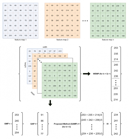
In the top-k max-pooling method, which is referred to as WEMP in this study and has been proposed in the field of natural language processing, each feature map has k outputs. These outputs are the highest activation values in the corresponding feature map. To the best of our knowledge, the WEMP method has not been applied to image classification problems in the past. In this study, the WEMP method has been adapted to a classification problem and its performance has been compared with other GP methods. Figure 1 shows the outputs of GAP, GMP, and WEMP obtained using 7×7 feature maps. It can be seen that the number of neurons is greatly reduced with GP methods.
Figure 1. Calculating the Global Max Pooling (GMP), Global Average Pooling (GAP), Word Embedding top-k Max-pooling (WEMP), and proposed Global Average of top-k Max-pooling (GAMP) methods for 7×7 resolution feature maps
In the WEMP and proposed GAMP methods, k=3 is taken.
3.2 Proposed method
In this section, the proposed GAMP method is discussed, taking into consideration the advantages and disadvantages of the commonly used GAP and GMP methods in CNN models. As previously mentioned, the GAP method produces an output by taking the average of all feature maps, but low activations can suppress high activations. The GMP method only takes the highest activation, which can weaken the model’s generalization ability. In the WEMP method, which was inspired by the scope of the study, the highest k activations are concatenated for each feature map; in other words, the feature map is not reduced to a single value and position information can be lost. In the proposed GAMP method, the average of the highest k activations for each feature map is taken to benefit from the advantages of the GAP and GMP methods and to produce a single value for each feature map. The average of the k highest activations in a feature map F can be represented mathematically as:
$F_0=F$ (3)
$E_1:=\left\{m \in M_0: m \geq \alpha \forall a \in F_0\right\}$ (4)
In Eq. (4), α represents each activation in feature map F0, and E1 represents the highest activation in feature map F0. Then, using Eq. (5), the highest activation value is excluded from the feature map.
$F_1:=F_0 \backslash E_1$ (5)
This process is repeated k times using Eqns. (6) and (7). At each step, the highest activation value is removed from the remaining values in feature map F0.
$E_{\mathrm{i+1}}:=\left\{m \in F_i: m \geq \alpha \forall a \in F_i\right\}$ (6)
$F_{\mathrm{i}+1}:=F_{\mathrm{i}} \backslash E_{\mathrm{i}+1}$ (7)
Finally, the average of the highest k activation is obtained using Eq. (8).
$r=\frac{1}{k} \sum_{i=0}^{i=k} E_{i+1}$ (8)
Eq. (8) represents the result obtained using the proposed method for the relevant activation map F0. These operations are applied independently for each feature map. Finally, a single activation value is obtained per feature map. Figure 1 shows an example of the proposed method with k=3 for 7×7 dimensional feature maps.
3.3 Datasets
The CIFAR-10 [30] dataset was created by the Canadian Institute for Advanced Research (CIFAR) and it is one of the most widely used image classification datasets. The dataset is designed to be challenging, with a small image size, a limited number of training samples, and a diverse set of classes. The CIFAR10 dataset consists of a total of 60000 images with 32×32 resolution RGB images, which are labeled into 10 classes. These classes are airplane, automobile, bird, cat, deer, dog, frog, horse, ship, and truck. The dataset is divided into 50000 training and 10000 test set. There are an equal number of samples for each class. In other words, there are 6000 images per class. There is no overlap between classes. The CIFAR10 dataset is a widely recognized benchmark in computer vision and machine learning, particularly in the area of deep learning. It is frequently utilized in the research literature as a standard evaluation set for proposing new algorithms and methods. Figure 2 (on the left) shows randomly selected examples from the CIFAR10 dataset and the corresponding classes. The CIFAR100 dataset consists of 100 classes with 600 images each and a total of 60000 images. The images in each class are divided into 500 training and 100 test. The image resolution is 32×32 like CIFAR10. The 100 classes in the dataset are also divided into 20 top classes. Therefore, a “fine” label that shows the class to which the image belongs and a “coarse” label that shows the top class to which it belongs are defined for each image. Figure 2 (on the right) shows randomly selected examples from the CIFAR100 dataset and the corresponding classes.
Figure 2. CIFAR10 (left) and CIFAR100 (right) random samples and their respective classes
3.4 Models
In this section, CNN models created for comparing GP methods are discussed. In this context, two different model architectures are established, Custom and VGG16-based [35]. The reason for conducting experimental studies on the two models is to observe the performance of the proposed method both in a model specifically established and in a model that provides state-of-the-art results on large datasets such as ImageNet [36].
First, a custom model was established to examine the performance of GP methods in a shallow model with randomly initialized weights. Table 1 gives other details about the model. The Custom model consists of convolution-batch normalization-ReLU layers with similar structures. 7×7 kernel sizes were used in the early layers since the number of kernels used was low, followed by 5×5 and then 3×3 kernel sizes in the later layers. Local max-pooling layers were used to reduce the resolution of the feature maps. 2×2 kernel sizes were used in these layers, and stride 2 was taken without overlapping. The 15×15 resolution feature maps at the output of the last layer were given as input to the GP layer. Finally, an FC layer was used to connect the neurons obtained per feature map to the classification layer. A softmax layer was used before the classification layer. Figure 3 shows the Custom model.
The architecture is symbolized based on the CIFAR10 dataset. The output layer consists of 100 neurons for the CIFAR100 dataset. The model was trained from scratch; no fine-tuning was applied.
Second, a VGG16-based model was used. The VGG16 model achieved the highest score in the ILSVRC-2014 competition with a test accuracy of 92.7% in the top-5 category on the ImageNet dataset in 2014. The VGG16 model has an architecture consisting of convolution blocks with 3x3 filters and 2×2 local max-pooling layers, using a consistent use of convolution and max-pooling layers throughout the architecture. The classification block includes 3 FC layers ending with a softmax layer. The main disadvantage of VGG16 is its high model capacity, with approximately 138 million parameters, making it slow to train, requiring a large amount of disk space and bandwidth, and making it inefficient. In this study, two modifications were performed to the VGG16 architecture. Firstly, the 3 FC layers in the classification layers were replaced with the GP layer. Secondly, an FC layer was used to create connections between the neurons obtained for each feature map and the classification layer.
In this context, if the number of filters was used in the fifth block equal to the number of classes, an additional FC layer would not be necessary. However, this approach was taken to preserve the basic architecture of the convolution layers in VGG16 and to use the pre-trained weights. Figure 4 shows the model created based on VGG16.
The first 5 blocks of the VGG16 model are used without modification. Pre-trained weights trained on the ImageNet dataset are used in these layers for all experimental settings. The 3 FC layers in the final layers of the VGG16 model are replaced with a GP layer. In the final layer, an FC layer is used to connect the neuron outputs obtained from the GP layer with the class layer. All weights are set to be trainable during the training phase.
Figure 3. Custom model
Figure 4. The architecture created is based on VGG16
Table 1. Custom model details. In the table, F represents the number of channel/feature map, W represents the width of the feature map, and H represents the height of the feature map
|
Input size (F, W, H) |
Layer |
Number of kernels |
Kernel size |
Stride |
Padding |
|
3×64×64 |
Conv2d + BatchNorm2d + ReLU |
16 |
7x7 |
1 |
2 |
|
16×62×62 |
Conv2d + BatchNorm2d + ReLU |
32 |
7x7 |
1 |
2 |
|
32×60×60 |
MaxPool2d |
- |
2x2 |
2 |
- |
|
32×30×30 |
Conv2d + BatchNorm2d + ReLU |
64 |
5x5 |
1 |
2 |
|
64×30×30 |
Conv2d + BatchNorm2d + ReLU |
128 |
5x5 |
1 |
2 |
|
128×30×30 |
MaxPool2d |
- |
2x2 |
2 |
- |
|
128×15×15 |
Conv2d + BatchNorm2d + ReLU |
256 |
3x3 |
1 |
1 |
|
256×15×15 |
Conv2d + BatchNorm2d + ReLU |
256 |
3x3 |
1 |
1 |
|
256×15×15 |
Global Pooling |
- |
15x15 |
- |
- |
|
256 |
Fully connected |
- |
- |
- |
- |
3.5 Training details
In this section, the training details of the models are given. Both the CIFAR10 and CIFAR100 datasets were trained for 50 epochs using the Custom model, as it has a low training time and is relatively shallow. The same experimental settings were used when comparing the methods; the same weight values and hyper-parameters were used for the model. The Adam [37] algorithm was used as the optimizer, with a batch size of 16 and a learning rate of 1−e3. Cross-Entropy Loss was used as the loss function. No preprocessing, e.g., data augmentation, or hyper-parameter optimization, e.g., learning rate decay, was performed that would cause randomness in the model. The model with the highest validation accuracy value during training was saved and the test score was examined. The VGG16-based model was trained for 20 epochs, as it is heavy, or in other words, has a long training time. The images in the custom model have been resized to a resolution of 64×64 due to the small size of the model, while in the VGG16 model, the images have been resized to a resolution of 224×224. The same training details were used for this model as for the Custom model. During the training phase of the VGG16-based model, the pre-trained values of the model trained on the ImageNet dataset were used. This model aims to compare the methods based on the feature maps with different resolutions given as input to the GP layer. For this purpose, in the VGG16-based model, 7x7 feature maps are formed at the output of the 5th block. To test at different resolutions, the entire 5th block was removed and the output of the 4th block was directly given to the GP layer. In this setting, the input to the GP layer was of 14x14 resolution.
In this section, the proposed GAMP method is experimentally compared with the commonly used GAP, GMP, and WEMP methods under different models, i.e., Custom and VGG16-based, and datasets, i.e., CIFAR10 and CIFAR100. First, the performance of the methods was examined using the Custom model (Figure 4) and the CIFAR10 dataset. In this architecture, the input to the GP layer is BxCxWxH, i.e., 16x512x15x15, where B represents the batch size, C represents the channel size, W represents the width of the feature map, and H represents the height of the feature map. The results obtained with this experimental setting are shown in the second column of Table 2. When GMP was used as the GP method in the Custom architecture, a test accuracy of 80.64% was obtained, and when GAP was used, a test accuracy of 82.49% was obtained. A comparison of the two methods showed that the GAP method achieved a test accuracy that was 1.85% higher on the CIFAR10 dataset. An analysis of the proposed GAMP method’s performance for various top-k values yielded test accuracies ranging from 81.98% to 83.78%. In the experimental studies carried out using the Custom architecture and the CIFAR10 dataset, the highest test accuracy of 83.78% was obtained when top-k=5 was taken with the proposed GAMP method. The proposed GAMP (top-k=5) method had 3.14% higher test accuracy when compared with GMP and 1.29% higher test accuracy when compared with GAP. The proposed method was inspired by the WEMP method, which is a well-known method in the field of word embedding. As previously mentioned, this method keeps all the highest activations and associates them with an FC layer for the next layer; in other words, the average of these activations is not taken. When the WEMP method was adapted to the CNN architecture and its performance was examined, a test accuracy of 81.19% was obtained. In this method, for a fair comparison, the test accuracy of proposed GAMP method at the top-k=5, where it achieved the highest performance, was examined. The WEMP method outperformed the GMP method by 0.55%, but it was behind the GAP method by 1.3%. When all the models were compared for this setting, the proposed GAMP method increased the test accuracy by 1.29% compared to the closest method, i.e., GAP. It is noteworthy in Table 2 that the accuracy values may vary based on the top-k value. Hence, to achieve the highest performance results, it is necessary to perform experiments with different top-k values. For example, an accuracy of 81.98% was obtained when top-k was set to 2. The accuracy improved to 83.78% when top-k was changed to 5 but decreased to 82.88% when top-k was set to 8.
Second, experimental studies were carried out using the Custom model and the CIFAR100 dataset to examine the performance of the methods on a different dataset. The results obtained with this experimental setting are shown in the third column of Table 2. It can be seen that the methods exhibit similar behavior to the previous setting. The GAP method yielded a test accuracy that was 1.04% higher than the GMP method when using the CIFAR100 dataset. When the performance of the proposed GAMP method was examined for different top-k values, test accuracies ranging from 46.12% to 49.01% were obtained. The proposed GAMP method achieved the highest test accuracy of 49.01% with top-k=9 in this experimental setting. The proposed GAMP (top-k=9) method provided a test accuracy that was 2.76% higher than the GMP method, 1.72% higher than the GAP method, and 2.54% higher than the WEMP method. In the WEMP method, top-k=9 was taken for a fair comparison with the proposed method. One point to be noted is that the success of the proposed GAMP method varies depending on different top-k values. For example, in the experiments on the CIFAR100 dataset, it was found that the proposed method was less successful than the other three methods when using top-k=4. In addition, it has been observed that the proposed method has achieved the highest performance on different datasets at different top-k values. Figure 5 depicts the training and validation accuracy graphs of the models that achieved the highest accuracy rates for the CIFAR10 and CIFAR100 datasets, respectively, for 50 epochs. It is clear that the accuracy rates are lower in the CIFAR100 dataset as the number of classes is higher.
Figure 6 shows the training, validation, and test accuracies of the proposed GAMP method on the CIFAR100 dataset for various top-k values. A notable increase in the training accuracy rate is observed when top-k=9, and the highest test accuracy is achieved in this setting.
In the following section of the study, the GP methods are compared using the popular CNN model, i.e., VGG16. Table 3 shows the results obtained using the CIFAR10 dataset. In this setting, an evaluation is also provided based on the resolutions of the feature maps given as input to the GP layer. In this context, first, the methods are compared using all the blocks of the VGG16 model (Figure 4), in which the resolutions of the feature maps are 7×7. The results for this setting are given in the second column of Table 3. The highest test accuracy rate of 76.26% was obtained by the proposed GAMP method with top-k=8. The success rates of the GMP, GAP and WEMP methods are 74.04%, 75.12%, and 74.26%, respectively. The proposed GAMP method provided a test accuracy increase of 1.14% compared to the best-performing GAP method. The highest score for the proposed method on the CIFAR10 dataset was obtained with top-k=5 using the Custom model and with top-k=8 using the VGG16-based model, indicating that the best scores can be obtained at different top-k values depending on the model. Therefore, to obtain the best scores using the proposed method on any dataset or model, it is necessary to examine the model performance for several top-k values. In the experimental studies, a model that provided the best scores for top-k<10 was obtained.
Table 2. Train, validation, and test accuracy for the Global Max Pooling (GMP), Global Average Pooling (GAP), Word Embedding top-k Max Pooling (WEMP), and proposed Global Average of top-k Max Pooling (GAMP) methods on the CIFAR10 and CIFAR100 datasets using the Custom model. In this model, the resolution of the feature maps given as input to the GP layer is 15×15
|
Models |
CIFAR10 |
CIFAR100 |
||||
|
|
Train Acc |
Val Acc |
Test Acc |
Train Acc |
Val Acc |
Test Acc |
|
GMP |
98.95 |
82.14 |
80.64 |
70.72 |
44.42 |
46.25 |
|
GAP |
99.66 |
82.88 |
82.49 |
69.10 |
47.42 |
47.29 |
|
WEMP |
99.47 |
81.40 |
81.19 |
72.22 |
44.60 |
46.47 |
|
GAMP (top-k=2) |
99.41 |
83.24 |
81.98 |
78.37 |
45.28 |
47.0 |
|
GAMP (top-k=3) |
99.53 |
83.02 |
82.03 |
70.40 |
45.72 |
46.78 |
|
GAMP (top-k=4) |
99.57 |
83.70 |
82.34 |
73.75 |
46.72 |
46.12 |
|
GAMP (top-k=5) |
99.65 |
84.02 |
83.78 |
70.13 |
47.04 |
48.10 |
|
GAMP (top-k=6) |
99.24 |
84.40 |
83.34 |
78.58 |
47.38 |
47.94 |
|
GAMP (top-k=7) |
99.67 |
83.68 |
82.88 |
73.08 |
46.32 |
48.56 |
|
GAMP (top-k=8) |
99.58 |
83.64 |
82.44 |
78.26 |
48.28 |
48.31 |
|
GAMP (top-k=9) |
99.35 |
83.84 |
82.68 |
96.17 |
48.26 |
49.01 |
|
GAMP (top-k=10) |
99.49 |
83.96 |
83.51 |
97.04 |
47.10 |
47.97 |
Figure 5. Training (blue) and validation (red) accuracy graphs of the models that performed best on the CIFAR10 (left) and CIFAR100 (right) datasets using the Custom model
Table 3. Train, validation, and test accuracy for Global Max Pooling (GMP), Global Average Pooling (GAP), Word Embedding top-k Max Pooling (WEMP), and the proposed Global Average of top-k Max Pooling (GAMP) methods using the VGG16-based model and the CIFAR10 dataset for feature maps of different resolutions. The resolution of the feature maps in the VGG16-based model is 7×7 (2nd column), and the resolution of the feature maps in the model that resulted from removing the 5th block in the VGG16 model is 14×14 (3rd column)
|
Models |
Dataset: CIFAR10 Model: VGG16-based Feature map size: 7×7 |
Dataset: CIFAR10 Model: VGG16-based without 5th block Feature map size: 14×14 |
||||
|
|
Train Acc |
Val Acc |
Test Acc |
Train Acc |
Val Acc |
Test Acc |
|
GMP |
86.13 |
74.96 |
74.04 |
92.50 |
71.72 |
69.90 |
|
GAP |
88.86 |
77.14 |
75.12 |
94.03 |
76.14 |
74.31 |
|
WEMP |
87.52 |
75.32 |
74.26 |
93.14 |
73.46 |
72.15 |
|
GAMP (top-k=2) |
87.18 |
74.26 |
73.04 |
92.43 |
76.36 |
73.40 |
|
GAMP (top-k=3) |
90.11 |
76.76 |
75.79 |
92.59 |
74.70 |
74.22 |
|
GAMP (top-k=4) |
84.75 |
74.92 |
74.08 |
92.86 |
76.57 |
72.16 |
|
GAMP (top-k=5) |
90.41 |
75.52 |
75.27 |
91.79 |
73.22 |
71.82 |
|
GAMP (top-k=6) |
88.59 |
75.58 |
74.37 |
90.18 |
74.24 |
72.73 |
|
GAMP (top-k=7) |
89.58 |
75.56 |
75.30 |
92.18 |
74.62 |
72.56 |
|
GAMP (top-k=8) |
90.04 |
75.80 |
76.26 |
93.45 |
75.28 |
71.94 |
|
GAMP (top-k=9) |
91.76 |
74.68 |
73.52 |
91.39 |
76.16 |
75.25 |
|
GAMP (top-k=10) |
92.42 |
75.26 |
73.65 |
93.72 |
74.30 |
74.04 |
Figure 6. Train, validation, and test accuracy performances for different top-k values using the Custom architecture and the CIFAR100 dataset
Figure 7. Performance of train, validation, and test accuracy for different top-k values using a VGG16-based architecture and the CIFAR100 dataset
Secondly, the performance of the models was evaluated while keeping the dataset the same (CI- FAR10) and increasing the resolution of the feature maps. In this context, the 5th block of the VGG16 model was removed, resulting in a change in the resolution of the feature maps given to the GP layers from 7×7 to 14×14. Table 3 (3rd column) shows the results obtained for this setting. The highest test accuracy rate of 75.25% was obtained by taking top-k=9 with the proposed GAMP method. The success of the GMP, GAP and WEMP methods is 69.90%, 74.31%, and 72.15%, respectively. In this setting, it is noteworthy that when the resolution of the feature maps is increased, representing the feature map with a single maximum value while ignoring the other values in the feature map significantly affects the performance of the model. In this context, the GAP method, which considers all values in the feature map, provides a 4.41% increase compared to the GMP method. However, the GAP method takes the average of all values in the feature map. This can cause low activation values to suppress high activation values, which can negatively affect the test performance of the model. The proposed GAMP method preserves the generalization ability of the model better by taking the average of the k-highest activations and increases the test accuracy value. Upon examination of Table 3, it has been observed that as the resolution of the feature vector input to the global pooling layer increases, the gap between the success of the global pooling methods increases. For example, when the performance of the GAP and GMP methods is examined for 7×7 resolution feature maps, the difference in performance is 1.08%, while for 14×14 resolution feature maps, the difference in performance between these methods is 4.41%. Experimental studies have similarly shown that the proposed GAMP method exhibits increased superiority over other models as the resolution increases. This indicates that feature maps are better represented with the proposed GAMP method.
Figure 7 shows the training, validation, and test accuracies of the model for different top-k values using a VGG16-based model and the CIFAR10 dataset. As can be seen, the performance of the proposed model varies according to the top-k value, as in the Custom model. For example, the performance of the proposed model for top-k=2 is behind the GMP, GAP, and WEMP methods.
In this study, a new GP method was proposed taking into account the advantages and disadvantages of the GMP and GAP methods, which are frequently used in deep neural networks. The proposed GAMP method enhances the model’s ability to generalize by maintaining high activation, resulting in improved classification performance on the test dataset. The proposed method was compared to other techniques in the same field using both a Custom model and a widely used CNN model (VGG16-based). The superiority of the proposed method was verified through experimental results. In this context, firstly, a comparison was made using the Custom model and the CIFAR10 dataset, and it was observed that the proposed GAMP (top-k=5) method has a test accuracy that is 3.14% higher than GMP and 1.29% higher than GAP. Secondly, in experimental studies using the same model architecture and CIFAR100 dataset, the proposed method (top-k=9) outperformed the closest-performing method, i.e., GAP, by 1.72%. Thirdly, the performance of the methods was evaluated when inputs of the different resolutions were given to the GP layer. In this direction, a VGG-based model architecture and the CIFAR10 dataset were utilized, and input to the GP layer was provided with feature vectors of resolution 7×7 and 14×14. Upon examination of the success of the methods, it was observed that the proposed method provides higher performance for both resolutions, and as the resolution increases, the difference in success between the methods increases. Then, the proposed method was compared with a similar approach referred to as WEMP for word embedding studies. In the WEMP approach, all of the highest k activations are kept and concatenated, while in our proposed method, the average of the highest k activations is taken. In order to make a comparison, the WEMP method was first adapted to the classification problem. Compared to WEMP, the proposed method provided a 2.59% increase for CIFAR10 and a 2.54% increase for CIFAR100. The success of the proposed method varies according to the selected k parameter. Intensive experiments showed that the best k value varies according to the model and dataset used. Therefore, the training of the model needs to be repeated for several k values. In general, it was observed that a model that outperforms the performance of other methods can be obtained when training is carried out for the k values in the range of [1-10]. In the continuation of the study, further experimental studies are planned to be carried out to make recommendations on the k parameter depending on the resolution of the feature map. The proposed method can be used to represent the values in a specific area with a single value in practice. In this study, the proposed method was used to reduce the dimension of the feature vector in CNNs and successful results were obtained. In the continuation of the study, the performance evaluation of resizing the images before giving them as input to CNNs is also planned.
[1] Sellami, A., Tabbone, S. (2022). Deep neural networks-based relevant latent representation learning for hyperspectral image classification. Pattern Recognition, 121: 108224. https://doi.org/10.1016/j.patcog.2021.108224
[2] Roger, V., Farinas, J., Pinquier, J. (2022). Deep neural networks for automatic speech processing: A survey from large corpora to limited data. EURASIP Journal on Audio, Speech, and Music Processing, 2022(1): 19. https://doi.org/10.1186/s13636-022-00251-w
[3] Montejo-Ráez, A., Jiménez-Zafra, S.M. (2022). Current approaches and applications in natural language processing. Applied Sciences, 12(10): 4859. http://doi.org/10.3390/books978-3-0365-4440-3
[4] Ozdemir, C., Gedik, M.A., Kaya, Y. (2021). Age estimation from left-hand radiographs with deep learning methods. Traitement du Signal, 38(6): 1565-1574. https://doi.org/10.18280/ts.380601
[5] Yetis, A.D., Yesilnacar, M.I., Atas, M. (2021). A machine learning approach to dental fluorosis classification. Arabian Journal of Geosciences, 14: 1-12. https://doi.org/10.1007/s12517-020-06342-2
[6] Lin, M., Chen, Q., Yan, S. (2013). Network in network. arXiv preprint arXiv:1312.4400. https://doi.org/10.48550/arXiv.1312.4400
[7] Krizhevsky, A., Sutskever, I., Hinton, G.E. (2017). Imagenet classification with deep convolutional neural networks. Communications of the ACM, 60(6): 84-90. https://doi.org/10.1145/3065386
[8] Ciresan, D.C., Meier, U., Masci, J., Gambardella, L.M., Schmidhuber, J. (2011). Flexible, high performance convolutional neural networks for image classification. In Twenty-second international joint conference on artificial intelligence. https://doi.org/10.5591/978-1-57735-516-8/IJCAI11-210
[9] Zeiler, M.D., Fergus, R. (2013). Stochastic pooling for regularization of deep convolutional neural networks. arXiv preprint arXiv:1301.3557. https://doi.org/10.48550/arXiv.1301.3557
[10] Sainath, T.N., Kingsbury, B., Mohamed, A.R., Dahl, G.E., Saon, G., Soltau, H., Beran, T., Aravkin, A.Y., Ramabhadran, B. (2013). Improvements to deep convolutional neural networks for LVCSR. In 2013 IEEE workshop on automatic speech recognition and understanding, pp. 315-320. http://doi.org/10.1109/ASRU.2013.6707749
[11] Akhtar, N., Ragavendran, U. (2020). Interpretation of intelligence in CNN-pooling processes: a methodological survey. Neural computing and applications, 32(3): 879-898. https://doi.org/10.1007/s00521-019-04296-5
[12] Wang, B., Zhou, X., Zhang, X. (2019). YNUWB at SemEval-2019 Task 6: K-max pooling CNN with average meta-embedding for identifying offensive language. In Proceedings of the 13th International Workshop on Semantic Evaluation, pp. 818-822. https://doi.org/10.18653/v1/S19-2143
[13] Graham, B. (2014). Fractional max-pooling. arXiv preprint arXiv:1412.6071. https://doi.org/10.48550/arXiv.1412.6071
[14] Yu, D., Wang, H., Chen, P., Wei, Z. (2014). Mixed pooling for convolutional neural networks. In Rough Sets and Knowledge Technology: 9th International Conference, RSKT 2014, Shanghai, China, pp. 364-375. http://doi.org/10.1007/978-3-319-11740-9_34
[15] Saeedan, F., Weber, N., Goesele, M., Roth, S. (2018). Detail-preserving pooling in deep networks. In Proceedings of the IEEE Conference on Computer Vision and Pattern Recognition, pp. 9108-9116. https://doi.org/10.1109/CVPR.2018.00949
[16] Sun, M., Song, Z., Jiang, X., Pan, J., Pang, Y. (2017). Learning pooling for convolutional neural network. Neurocomputing, 224: 96-104. https://doi.org/10.1016/j.neucom.2016.10.049
[17] He, K., Zhang, X., Ren, S., Sun, J. (2015). Spatial pyramid pooling in deep convolutional networks for visual recognition. IEEE Transactions on Pattern Analysis and Machine Intelligence, 37(9): 1904-1916. https://doi.org/10.1109/TPAMI.2015.2389824
[18] Cui, Y., Zhou, F., Wang, J., Liu, X., Lin, Y., Belongie, S. (2017). Kernel pooling for convolutional neural networks. In Proceedings of the IEEE conference on computer vision and pattern recognition, pp. 2921-2930. https://doi.org/10.1109/CVPR.2017.325
[19] Wang, F., Huang, S., Shi, L., Fan, W. (2017). The application of series multi-pooling convolutional neural networks for medical image segmentation. International Journal of Distributed Sensor Networks, 13(12): 1550147717748899. https://doi.org/10.1177/1550147717748899
[20] Sermanet, P., Chintala, S., LeCun, Y. (2012). Convolutional neural networks applied to house numbers digit classification. In Proceedings of the 21st international conference on pattern recognition (ICPR2012), pp. 3288-3291. https://doi.org/10.48550/arXiv.1204.3968
[21] Wu, H., Gu, X. (2015). Max-pooling dropout for regularization of convolutional neural networks. In Neural Information Processing: 22nd International Conference, ICONIP 2015, Istanbul, Turkey, November 9-12, 2015, Proceedings, Part I 22, pp. 46-54. http://doi.org/10.1007/978-3-319-26532-2_6
[22] Song, Z., Liu, Y., Song, R., Chen, Z., Yang, J., Zhang, C., Jiang, Q. (2018). A sparsity-based stochastic pooling mechanism for deep convolutional neural networks. Neural Networks, 105: 340-345. https://doi.org/10.1016/j.neunet.2018.05.015
[23] Tong, Z., Aihara, K., Tanaka, G. (2016). A hybrid pooling method for convolutional neural networks. In Neural Information Processing: 23rd International Conference, ICONIP 2016, Kyoto, Japan, pp. 454-461. http://doi.org/10.1007/978-3-319-46672-9_51
[24] Shahriari, A., Porikli, F. (2017). Multipartite pooling for deep convolutional neural networks. arXiv preprint arXiv:1710.07435. https://doi.org/10.48550/arXiv.1710.07435
[25] Kumar, A. (2018). Ordinal pooling networks: for preserving information over shrinking feature maps. arXiv preprint arXiv: 1804.02702. https://doi.org/10.48550/arXiv.1804.02702
[26] Kolesnikov, A., Lampert, C.H. (2016). Seed, expand and constrain: Three principles for weakly-supervised image segmentation. In Computer Vision–ECCV 2016: 14th European Conference, Amsterdam, The Netherlands, pp. 695-711. http://doi.org/10.1007/978-3-319-46493-0_42
[27] Williams, T., Li, R. (2018). Wavelet pooling for convolutional neural networks. In International conference on learning representations. https://openreview.net/forum?id=rkhlb8lCZ
[28] Rippel, O., Snoek, J., Adams, R.P. (2015). Spectral representations for convolutional neural networks. Advances in neural information processing systems, 28. https://doi.org/10.48550/arXiv.1506.03767
[29] Wang, Z., Lan, Q., Huang, D., Wen, M. (2016). Combining FFT and spectral-pooling for efficient convolution neural network model. In 2016 2nd International Conference on Artificial Intelligence and Industrial Engineering (AIIE 2016), pp. 203-206. https://doi.org/10.2991/aiie-16.2016.47
[30] Krizhevsky, A., Nair, V., rey Hinton, G. (2014). e CIFAR-10 dataset.
[31] Atas, I., Ozdemir, C., Atas, M., Dogan, Y. (2022). Forensic dental age estimation using modified deep learning neural network. arXiv preprint arXiv:2208.09799. https://doi.org/10.48550/arXiv.2208.09799
[32] Hinton, G.E., Srivastava, N., Krizhevsky, A., Sutskever, I., Salakhutdinov, R.R. (2012). Improving neural networks by preventing co-adaptation of feature detectors. arXiv preprint arXiv:1207.0580. https://doi.org/10.48550/arXiv.1207.0580
[33] Lee, C.Y., Gallagher, P.W., Tu, Z. (2016). Generalizing pooling functions in convolutional neural networks: Mixed, gated, and tree. In Artificial intelligence and statistics, pp. 464-472. https://doi.org/10.48550/arXiv.1509.08985
[34] LeCun, Y. (1989). Generalization and network design strategies. Connectionism in perspective, 19(143-155): 18.
[35] Simonyan, K., Zisserman, A. (2014). Very deep convolutional networks for large-scale image recognition. arXiv preprint arXiv:1409.1556. https://doi.org/10.48550/arXiv.1409.1556
[36] Deng, J., Dong, W., Socher, R., Li, L. J., Li, K., Li, F.F. (2009). Imagenet: A large-scale hierarchical image database. In 2009 IEEE conference on computer vision and pattern recognition, pp. 248-255. http://doi.org/10.1109/CVPR.2009.5206848
[37] Kingma, D.P., Ba, J. (2014). Adam: A method for stochastic optimization. arXiv preprint arXiv:1412.6980. https://doi.org/10.48550/arXiv.1412.6980