Muhammad Shehzad Hanif*![]() | Muhammad Bilal
| Muhammad Bilal![]() | Abdullah Saeed Balamash
| Abdullah Saeed Balamash![]() | Ubaid M. Al-Saggaf
| Ubaid M. Al-Saggaf![]()
© 2023 IIETA. This article is published by IIETA and is licensed under the CC BY 4.0 license (http://creativecommons.org/licenses/by/4.0/).
OPEN ACCESS
A two-stage framework for crowd anomaly detection in single-scene or scene-dependent surveillance videos is proposed in this article. The first stage generates several hypotheses corresponding to potential anomalous regions in a video frame and the second stage verifies them to reduce false alarms and identifies crowd anomalies. In the hypotheses generation stage, spatial and temporal derivatives are computed for each video frame and a saliency detector employing Hypercomplex Fourier Transform (HFT) is used to generate a saliency map. A threshold is applied to the saliency map to generate potential anomalous regions in the form of connected components. For each connected component, a set of 4 statistical features are computed and fed to the second stage which employs a Gaussian Mixture Model (GMM) as a verification method to yield the final crowd anomalies in the frame. The effectiveness of the proposed framework has been shown through results obtained on the UCSD anomaly detection benchmark dataset which contains two subsets namely Ped1 and Ped2 with a total of 48 test videos (9210 frames). Both frame-level and pixel-level anomaly detection results are provided using the widely recognized evaluation criterion in the domain and compared with the state-of-the-art methods. The experimental results show that the proposed framework obtains comparable results against the state-of-the-art methods.
crowd anomaly detection, gaussian mixture model, hypercomplex Fourier transform, visual saliency detection
Automatic crowd analysis is an open research problem and has extensive applications in the fields of crowd safety and surveillance, crowd management, event detection, anomaly detection and design of smart environments for public gatherings, etc. [1, 2]. However, the task is challenging due to the inherent complexity as crowd dynamics are not deterministic and cannot be predicted in advance. Researchers working in the domain of computer vision and pattern recognition are interested in the development and deployment of robust and sophisticated algorithms and techniques to perform visual crowd analysis where video streams are the only available inputs.
Crowd anomaly detection is one of such tasks where the objective is to detect appearances and/or motion patterns deviating from the prevalent appearances and/or motion patterns in crowd videos. However, crowd anomaly detection is not trivial as types of anomalies are not known in advance and their occurrences are rare. Moreover, they may occur at any instant with no fixed duration in a video. Therefore, it is desired to detect anomalies both spatially and temporally in videos. Figure 1 shows three examples from the UCSD anomaly detection benchmark dataset used in this work where “cyclist”, “skater” and “vehicle” are anomalous regions/objects in the scenes as they appear on the pedestrian pathway. To handle all sorts and categories of anomalies, a typical setting is to train a model on a set of non-anomalous or normal video frames (train set) and then the learned model is applied to the anomalous frames (test set). It is also interesting to note that in many earlier works [3-13], crowd anomaly detection is either considered as scene-dependent (train and test sets contain the same scene) or scene-independent (train and test set contain different scenes) task. It has been argued by Ramachandra et al. [3] that the crowd anomaly detection is indeed a scene-dependent task as it is the only realistic scenario in surveillance videos for real-world applications. Thus, in this work, a crowd anomaly detection task has been considered in scene-dependent (also known as single-scene) surveillance videos. The proposed framework has two stages where the first stage is composed of a saliency detector responsible for generating a saliency map indicating potential anomalous regions in a video frame. The second stage subsequently validates these anomalous regions. The proposed saliency detector is influenced by the works of Li et al. [14] and Guo and Zhang [15] on computational of visual saliency in the frequency domain. Specifically, spatial and temporal gradients are extracted from a video frame and Hypercomplex Fourier Transform (HFT) based saliency detection method of [14, 15] is applied. It is important to note that the authors in [14] applies the HFT based saliency detector to static color images while the work [15] is related to image and video compression. Therefore, the saliency detector for generating potential anomalous regions has not been proposed earlier in the literature. It is pertinent to mention to the reader that a closely related work using frequency domain-based saliency detector for crowd anomaly detection [16] is based on spectral residual approach of Hou and Zhang [17] which is in theory different than the proposed technique and has been proven to be inferior to the HFT based saliency detector by Li et al. [14]. In the next step, the saliency map is subject to a threshold to generate a binary map and connected components are determined. In the verification stage, four statistical features are computed from connected components containing significant motion and the corresponding regions in the saliency map, and a generative model in the form of a Gaussian Mixture Model (GMM) is learned. Normal (non-anomalous) frames of the train dataset are used to train the GMM. When applied to the test dataset, the GMM based generative model outputs low likelihood scores for anomalous regions. The verification stage, in the proposed work, is a supervised learning approach contrary to the hypotheses generation stage and helps in reducing the false alarms in the saliency map. The proposed framework is verified for functionality on the public domain UCSD anomaly detection benchmark dataset. Anomaly detection results on frame-level and pixel-level are provided in this work and are quite promising. The proposed framework achieves comparable performance when compared to existing methods using the widely recognized evaluation criterion in the domain. The main contributions of this work can be summarized as follows:
Figure 1. (a)-(c) Examples of crowd anomaly in the UCSD dataset
The rest of the article is structured as follows: a review of relevant techniques and methods for crowd anomaly detection is presented in section 2. The proposed framework is detailed in section 3 where both hypotheses generation and validation stages are discussed. The experimental results along with dataset description and implementation details are presented in section 4. Finally, conclusions and future directions are described in section 5.
Crowd anomaly detection in surveillance videos has been an active area of research for more than a decade. In general, methods in the literature in this field have focused on these three axes: efficient representation of motion patterns, anomaly modeling and classification techniques. A concise review of the related and recent works in the field of crowd anomaly detection is presented next.
In a seminal work [8], Mahadevan et al. propose to encode appearance and dynamics of motion patterns in a joint manner with the help of dynamic textures. Abnormality detection is accomplished at both spatial (pixel) and temporal (frame) levels. For temporal detection of anomalies, dynamic textures are modeled using Gaussian mixture models (GMMs) on spatiotemporal slices around a frame and a saliency map is generated. Spatiotemporal slices are generated by dividing the image in non-overlapping blocks of pixels and extending them in the time axis. The spatial detection is based on computation of center-surround saliency with the help of GMMs at a certain block in a frame and its spatial neighbors. In a follow-up work by the same team of researchers [18], the dynamic textures based approach is further refined by fusion of temporal and spatial saliency maps at multiple spatial scales. Lu et al. [19] propose to divide the frame into non-overlapping blocks of pixels at multiple scales and compute spatial and temporal derivatives. A sparse combination learning scheme is proposed to model reconstruction of blocks with the help of a dictionary which is trained on the normal frames of train set. During the test, reconstruction scores are employed to categorize blocks. Wang and Xu [4] employ the wavelet transform to spatiotemporal slices around a frame to encode the texture information present in the scene. These features are extracted at different locations of the frame in the sliding window fashion and assumed to follow a Gaussian distribution. A generative model is learnt from normal video frames in the train set to describe normality. During the test, the dissimilarity between the texture features on a test frame and the model is used as a measure to detect anomaly. Colque et al. [20] present a descriptor called HOFME using the histogram of optical flow orientation and magnitude and entropy computed on the spatiotemporal slices at fixed locations in a frame. The HOFME descriptors are computed on normal frames of the train dataset. To detect anomaly in a test video, the HOFME descriptors are computed and a nearest neighbor classifier is employed. Sun et al. [9] propose a visual saliency detector using a dissimilarity measure between a spatiotemporal block at a position in a frame and its neighboring spatiotemporal blocks. The L1 distance metric is employed to compute the dissimilarity in this work. In addition to the saliency map, the authors propose to compute a motion disorder map using block-based difference of motion vectors between frames. A linear combination of these two maps results in a map where the higher values represent anomalous regions in the frame.
Adam et al. [12] propose fixed-position monitoring for detection of anomaly in video frames. Optical flows at fixed positions (or regions) in the frames are modeled by a probabilistic model. Image regions with low likelihood scores in test frames are considered anomalous. A social force model based on optical flow fields is proposed in the study of Mehran et al. [11]. Optical flow of a certain region in a frame is compared with the average optical flow of its neighbors and this interaction is modeled with the help of bag-of-words. Test regions with low likelihood are considered anomalous ones. Ryan et. al. [10] present a texture encoding scheme using co-occurrence matrices computed on the optical flow fields. A measure known as uniformity is computed using the spatiotemporal slices extracted at all locations of a video frame to encode the appearance and motion patterns. A Gaussian mixture model (GMM) is then trained using the uniformity features on the normal video frames of the train set. Likelihood between the uniformity features extracted on the spatiotemporal slices of the test frames and the GMM model is used to determine anomalous frames. Wang et al. [16] employ an unsupervised learning approach based on a visual saliency model for crowd anomaly detection. The visual saliency model is based on the spectral residual approach proposed in the study of Hou and Zhang [17]. A single saliency score per frame is computed by simple accumulation of all scores in a saliency map across rows and columns. Finally, frames having saliency scores higher than a threshold are categorized as anomalous frames. It is important to note that only frame-level anomaly detection results are reported in the research works by Ryan et al. [10] and Wang et al. [16], and performances of the proposed approaches for spatial localization of anomalies have not been presented.
Antić and Ommer [21] propose to extract foreground information with the help of a background subtraction-based method. Spatial and temporal derivatives are computed to encode appearance and motion patterns of foreground objects. Support vector machine (SVM) based classification method is used to detect anomalies at both frame and pixel levels. Similarly, to the above-mentioned work, Bansod and Nandedkar [7] present a three-stage approach to detect anomalies in single-scene videos. They use background subtraction as a first stage to extract all moving objects in a frame followed by blob detection and feature extraction. In the feature extraction stage, seventeen features based on optical flow magnitude and blobs attributes are computed. K-means clustering algorithm is then used to generate clusters to represent non-anomalous characteristics of moving objects in the train set. During the test, the blob features from test frame are compared with the centers of the clusters using L1 distance metric. The dissimilar blobs are denoted as anomalous regions in the frame.
In most recent works, deep convolutional neural networks (CNNs) have been employed to detect anomalies in crowd surveillance images owing to their superior performance in other computer vision tasks like object detection, image segmentation, image recognition, object tracking, etc. [22]. Ionescu et al. [23] employ pre-trained VGG- model [24] to encode appearance using conv5 layer of the network. Moreover, spatiotemporal derivates are used to encode motion patterns. K-means clustering and one-class SVM based model is trained on normal frames of train set to represent normal behavior. A simple threshold on SVM output yields frame-level anomaly detection. CNN based autoencoders are widely employed in anomaly detection. Tran and Hogg [5] employ a winner-takes-all convolutional autoencoder for scene reconstruction. Further, one-class SVM is trained on motion features of autoencoder to model normal motion behavior from normal frames of the train set. On test frames, the output of one-class SVM is considered as the abnormality score. Xu et al. [6] propose variational autoencoder for appearance and motion encoding. A GMM based model trained on the latent feature space of proposed autoencoder is then used to detect anomalies at both pixel and frame levels. In a closely related work [25], two variational autoencoders are proposed to encode appearance and motion patterns. Then, a GMM based model is trained on the combined feature space, is used to detect anomalous frame and spatial localization of anomalous regions in the frame.
It is evident from the above literature review that the appearance and motion patterns are generally encoded with the help of spatiotemporal slices and optical flow. But both representations are indeed noisy and unstable over the length of a video [26]. It is also apparent that visual saliency-based methods are commonly employed for anomaly detection in videos. However, a few works like [16] have employed frequency domain-based methods for visual saliency computation for anomaly detection in crowd surveillance videos. Therefore, in this work, the focus is on frequency domain based visual saliency computation to complement the existing methods. Additionally, a verification scheme to validate the potential anomalous regions in the saliency map is proposed contrary to many works where a simple threshold on the saliency map is applied to yield anomalous objects.
In this section, the details of the proposed two-stage framework for crowd anomaly detection consisting of hypotheses generation stage and verification stage are presented. In summary, the hypotheses generation stage is a saliency detector employing Hypercomplex Fourier Transform (HFT) and combines spatiotemporal derivatives. The verification stage is a Gaussian Mixture Model (GMM) employed to validate the potential anomalous regions in the saliency map. All blocks of the proposed framework have been depicted in Figure 2.
Figure 2. The block diagram of the proposed framework
3.1 Hypercomplex Fourier transform
In image processing, the traditional Fourier transform takes real valued pixel intensities as input. For multichannel images such color images, the Fourier transform is usually applied to each channel individually and does not combine multichannel information. Ell and Sangwine [27] proposed a variant of Fourier transform called Hypercomplex Fourier Transform (HFT) by representing the color image in the quaternion form. Following their seminal work, subsequent works have employed HFT for various applications including visual saliency computation [14, 28] and image and video compression [15].
In general, a hypercomplex image using quaternion representation is written as:
$f(x, y)=q_1+q_2 i+q_3 j+q_4 k$, (1)
where, q1, q2, q3 and q4 are real numbers and i, j, k satisfy i2=j2=k2=ijk=-1.
Now, the discrete HFT pair for a hypercomplex image of size M×N can be written as:
$\mathcal{F}(u, v)=\frac{1}{\sqrt{M N}} \sum_{x=0}^{N-1} \sum_{y=0}^{M-1} e^{-\rho 2 \pi\left(\frac{x u}{N}+\frac{y v}{M}\right)} \, f(x, y)$ (2)
$f(x, y)=\frac{1}{\sqrt{M N}} \sum_{u=0}^{N-1} \sum_{v=0}^{M-1} e^{{\rho 2 \pi\left(\frac{x u}{N}+\frac{y v}{M}\right)}{\mathcal{F}}(u, v)}$ (3)
where, ρ is a unit pure quaternion and ρ2=-1.
It is important to note that HFT is a generalization of traditional Fourier transform built on the generalization of Euler’s formula: eμθ=cos(θ)+μsin(θ). In general, the input to the HFT can be considered as a multi-channel or vector-valued signal and the HFT makes use of correlations between the channels to express the relationship between them in the frequency domain. The ability to express mutual information between channels makes it extremely useful in computer vision applications where it is customary to compute multiple features from the input image. In this work, the HFT has been applied to extract salient information in spatial and temporal derivatives of images as discussed in the next section. Moreover, like traditional Fourier transform, the HFT has similar properties like linearity, scaling, time reversal, modulation, convolution, etc., and are expressed with transform pairs but applied to multi-channel or vector-valued signals. The focus of this work is on the application of the HFT for saliency detection. For complete derivation and properties of HFT, more information may be found in Ref. [29].
3.2 Saliency detector
In crowd anomaly detection, the objective is to identify irregular appearance and motion patterns which are not dominant in a video frame. In other words, the objective is to detect salient regions in the video frame caused by the appearance and motion of anomalous objects. The proposed saliency detector is influenced by the work on visual saliency computation in natural images by Li et al. [14]. For a multi-channel or multi-feature image, the input to HFT is defined as follows:
$f(x, y)=\alpha_1 f_1+\alpha_2 f_2 i+\alpha_3 f_3 j+\alpha_4 f_4 k$, (4)
where, α1 to α4 are weights and f1 to f4 are different channels or features of input image.
Let I(x, y, t) denote a video frame at time instant t, spatial derivates Ix and Iy and temporal derivative It are computed numerically using finite difference approximation. The spatiotemporal derivates $\left[I_x \triangleq \frac{\partial I}{\partial x}, I_y \triangleq \frac{\partial I}{\partial y}, I_t \triangleq \frac{\partial I}{\partial t}\right]$ serve as the multi-feature input to HFT with f2=Ix, f3=Iy, and f4= It in the form of a pure quaternion with f1=0. The selected values of α1=0, α2=0.25, α3=0.25 and α4=0.5 in this work for all experiments give equal weights to spatial and temporal derivatives. For saliency computation, the HFT of the quaternion f(x, y) using Eq. (2) is computed which is also a quaternion and corresponds to the frequency domain representation of f(x, y). Let A(u, v), ϕ(u, v) and β(u, v) denote amplitude spectrum, phase spectrum and eigenaxis spectrum respectively, the HFT can be written as a quaternion and corresponding polar forms as:
$\mathcal{F}(u, v)=F_1+F_2 i+F_3 j+F_3 k=A(u, v) e^{\beta(u, v) \phi(u, v)}$ (5)
The amplitude A(u, v), phase ϕ(u, v) and eigenaxis β(u, v) spectrums are computed using the quaternion algebra in the following way:
$\begin{gathered}A(u, v)=|\mathcal{F}(u, v)|=\sqrt{F_1^2+F_2^2+F_3^2+F_4^2} \\ \beta(u, v)=\left(F_2 i+F_3 j+F_4 k\right) / \sqrt{F_2^2+F_3^2+F_4^2} \\ \phi(u, v)=\tan ^{-1}\left(\sqrt{F_2^2+F_3^2+F_4^2} / F_1\right)\end{gathered}$ (6)
where, |. | denote the modulus of quaternion.
The amplitude spectrum A(u, v) contains critical information about the scene. It is noteworthy that it contains information regarding both salient and non-salient regions due to the global nature of the transform and is therefore filtered using a lowpass filter with suitable scale to compute saliency while phase and eigenaxis spectrums are not modified. For this purpose, a set of Gaussian lowpass filters of the following type is proposed by Li et al. [14].
$g(u, v, l)=G e^{-\left(u^2+v^2\right) /\left(0.25 * 2^{2 l-1}\right)} \, \, \, \, \, , l=1, \ldots, L$ (7)
where, l is the scale parameter; L is the number of scales and is equal to ⌈log2 min(M,N)⌉+1 for a frame size of M×N; G is the normalization factor such that the sum of filter kernel is 1.
The filtered amplitude spectrum denoted as $\tilde{A}(u, v, l)$ is computed using the convolution of amplitude spectrum with the set of Gaussian filters g. Mathematically,
$\tilde{A}(u, v, l)=A(u, v) * g(u, v, l), \quad l=1, \ldots, L$ (8)
The above equation generates multiple amplitude spectrums corresponding to different scales. The objective of filtering is to suppress the non-salient regions while the scale-based filtering preserves the salient regions. Following [14], a set of saliency maps using filtered amplitude spectrums, unchanged phase and eigenaxis spectrums and inverse HFT (Eq. (3)) is computed as follows:
$\tilde{S}(x, y, l)=\left|\mathcal{F}^{-1}\left[\tilde{A}(u, v, l) e^{\beta(u, v) \phi(u, v)} \, \, \, \right]\right |^2, l=1, \ldots, L$ (9)
In the next step, the best scale (l*) for the saliency from the L possible scales, is selected using the entropy-based criterion of Li et al. [14]. According to this criterion, saliency map having the lowest entropy is the best where entropy is computed using the histogram of saliency map. The final saliency map S(x, y) is computed by applying a Gaussian filter h of fixed scale to the selected saliency map. Mathematically, the operation can be written as:
$S(x, y)=h * \tilde{S}\left(x, y, l^*\right)$ (10)
The objective of applying the Gaussian filter h is to combine under-segmented regions in the saliency map for the hypotheses generation which are further validated in the verification stage. The default scale of the filter is set to 0.05×N following the work of Li et al. [14] in the experiments. Though the proposed saliency detector follows the method of Li et al., it has been employed for anomaly detection using spatiotemporal derivates owing to the nature of the task at hand contrary to intensity and color-based features employed by them for visual saliency computation in natural scene images.
3.3 Verification method
The saliency detector described in the previous section yields a single saliency value for each pixel in a frame i.e., S(x, y) in an unsupervised manner. The higher values in the saliency map are the potential anomalous pixels belonging to an object. Therefore, to capture the characteristics of an anomalous object in a frame, a threshold (γ) must be applied to obtain a segmented saliency map (using the generated binary map). However, the selection of this threshold is dependent on the scene content and range of saliency values are not known in advance. Moreover, a local estimate is required to respect the real-time constraint in surveillance video streams. A local heuristic based on maximum of the saliency values in a map is proposed in this work. Specifically, γ=0.5×max(S(x,y)) has been set in all the experiments. The generated hypotheses in the form of segmented saliency map may contain false alarms and therefore, a verification method is required to validate them.
Recall that the threshold (γ) produces a binary image from the saliency map. Connected components in the binary image using 8-connectivity are determined for further analysis. Connected components with an area less than 15 pixels and more than 1/4th of the frame size, are filtered as connected components of this size do not represent anomalous regions. Moreover, connected components with significant motion obtained using temporal derivative It are considered. Next, for each connected components defined by its bounding box and by using the corresponding saliency values, four statistical features namely mean, variance, maximum and entropy of saliency values are computed to generate a 4-dimensional feature vector z.
The train set is composed of normal frames. The four statistical features are extracted from the complete train set and are modeled by a GMM (Eq. (11)) by assuming that the features follow 4-dimensional multi-modal Gaussian distribution $\mathcal{N}\left(\boldsymbol{\mu}_c, \boldsymbol{\Sigma}_c\right)$ with mean vector μc, and covariance matrix Σc. In the proposed implementation, full-covariance matrix is used. The task of learning is to compute the mixture coefficients πc, mean vectors μc and covariance matrices Σc using the given feature set $\left\{\boldsymbol{z}_n\right\}_{n=1}^{N_f}$ where Nf is total number of examples. The features are standardized to have zero mean and unit variance before the training. The GMM is initialized with K-Means++ algorithm and trained using the Expectation-Maximization algorithm [30].
$p\left(\mathbf{z}_n\right)=\sum_{c=1}^C \pi_c \mathcal{N}\left(\mathbf{z}_n \mid \boldsymbol{\mu}_c, \mathbf{\Sigma}_c\right)$ (11)
One of the important considerations during the training of GMM is the number of Gaussian components (C) in the mixture. In general, it is not trivial to know the number of Gaussian components (C) in the mixture for a given task. Moreover, many components in the mixture lead to overfitting. To find the optimal value of C, the Bayesian Information Criterion (BIC) for model selection [30] is employed. In general, a lower BIC value corresponds to best fitted model.
In the test phase, the trained GMM model is applied to features extracted from the connected components from saliency map of a test frame and probability density function (pdf) p(zn) using Eq. (11) is computed. Connected components with small pdf values correspond to the anomalous regions as the GMM model is trained to learn normal appearance and motion behaviors. The output of this stage is an anomaly score map.
In this section, the experimental results of the proposed framework for hypotheses generation and verification framework have been given. Additionally, the description of the benchmark dataset, evaluation criteria and implementation details are also presented.
4.1 UCSD anomaly dataset
In this work, the most commonly used single-scene video dataset for crowd anomaly detection known as UCSD anomaly dataset has been considered. It is available online at http://www.svcl.ucsd.edu/projects/anomaly/dataset.html and was introduced by Mahadevan et al. [8]. The dataset is composed of two subsets: Ped1 and Ped2. Each subset records a pedestrian walkway scenario with a single stationary camera in gray scale and the crowd density is not fixed. Pedestrians are moving towards or away from the camera in Ped1 while they are moving parallel to the camera plane in Ped2. Common occurring anomalous events are categorized as “bikers”, “cart”, “wheelchair”, “skaters”, “walk across” and “others”. All anomalies occur naturally and are not staged. There are a total of 6800 frames in 34 train videos and 7200 frames in 36 test videos in Ped1. In other words, each video in subset is composed of 200 frames. Moreover, the frame size is 158 x 238 pixels. The subset Ped2 contains a total of 2550 frames in 16 train videos and 2010 frames in 12 test videos. The number of frames varies from 120 to 180 in videos of the subset and the frame size is 240 x 360 pixels. Both frame-level (indices of anomalous frames) and pixel level (binary maps) ground truths are provided in the dataset. In its initial version of the dataset, pixel-level ground truth for Ped1 was available only for 10 test videos. Later, Antić and Ommer [21] completed the pixel-level ground truth. In this work, results using the complete pixel-level ground truth are reported.
4.2 Evaluation criteria
There are two widely used criteria for performance evaluation of an anomaly detector: 1) frame-level criterion; 2) pixel-level criterion. In both criteria, at a given threshold for the output of detector (anomaly score map) true positive rate (TPR) and false positive rate (FPR) are computed using Eq. (12). The threshold is varied to generate Receiver Operating Characteristic (ROC) curve using TPR and FPR. To summarize the ROC curve, two metrics namely Area Under the Curve (AUC) and Equal Error Rate (EER) are computed.
$\begin{aligned} & \text { TPR }=\frac{\text { number of true positives frames }}{\text { total number of positive frames }} \\ & \text { FPR }=\frac{\text { number of false positives frames }}{\text { total number of negative frames }}\end{aligned}$ (12)
In frame-level criterion, a frame is considered as anomalous if a single pixel in the score map is marked as anomalous. Using this principle, true positives and false positives are counted with the help of ground truth and TPR and FPR are computed. In other words, the frame-level criterion deals with the temporal detection of anomalous events and does not take into consideration the spatial localization of anomalous objects in a frame.
Pixel-level criterion compliments the frame-level criterion and measures the accuracy of detector by considering the spatial localization of anomalous objects in a frame. To qualify as a true positive, a frame must be anomalous according to the ground truth and have at least 40% pixels marked as anomalous in the score map compared against the pixel-level ground truth. A frame is considered as a false positive if a frame is normal according to the ground truth and has a single pixel marked as anomalous in the score map. After counting the true and false positives, TPR, FPR, AUC and EER are computed.
4.3 Detection results
As mentioned earlier, the saliency detector in the proposed framework indicates potential anomalous regions in its output map. To validate the potential regions, connected components and statistical features from the output map are computed as explained in section 3.3. Next, a GMM is trained using the normal frames in the train set. For Ped1 and Ped2 set, a total of 6078 and 1062 connected components are extracted. To obtain optimal number of components (C) in the mixture, GMM models are trained by varying the number of components from 2 to 20 and model selection using BIC criterion is performed. The maximum number of iterations for training the GMM is set to 1000 in the experiments. The final GMM models are composed of 6 components each for Ped1 and Ped2 subsets.
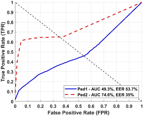
The quantitative results in terms of ROC curves of the proposed framework are shown in Figures 3 and 4. To summarize the ROC curves, the AUC and EER metrics are used for frame-level and pixel-level criteria. The frame-level AUC for Ped1 and Ped2 are 67.7% and 84.1% respectively while the corresponding EER scores are 37.6% and 22.7%. The pixel-level AUC for Ped1 and Ped2 are 49.3% and 74.6% respectively with 53.7% and 35% as EER scores.
Figure 3. Frame-level ROC curves on UCSD dataset
Figure 4. Pixel-level ROC curves UCSD dataset
Quantitative results with five existing methods are reported in Tables 1 and 2. All methods listed for the comparison employ statistical models like ours to have a fair comparison. Considering the frame-level criterion (see Table 1), the proposed framework achieved competitive AUC and EER compared to Fixed-Location Monitors [12] and Social Force [11] on Ped1 subset. But the performance is superior to these methods on Ped2 subset by more than 20%. Moreover, the results of the proposed framework is comparable to Mixture of Dynamic Textures (MDT) [18] and Foreground Occupancy and Optical Flow (FOOF) [13] on Ped2 subset. The proposed framework lags behind Histogram of Magnitude and Momentum (HoMM) [7] by 14.6% on Ped1 and 10% on Ped2 in terms of AUC. Considering the pixel-level criterion (see Table 2), the performance of the proposed framework is better than Fixed-Location Monitors, Social Force and MDT on both Ped1 and Ped2 subsets while competitive results are obtained compared to FOOF on Ped2 subset. The HoMM achieves the best results in terms of AUC and EER on both subsets. Compared to the proposed framework, the HoMM exceeds by 22.2% on Ped1 subset and 9.3% on Ped2 subset in terms of AUC.
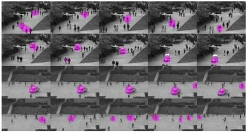
Qualitative results on Ped1 and Ped2 subsets are also provided in Figure 5. Each row in the figure shows the detection of anomalies (biker, cart, skater) in different frames of the subsets. It can be observed that the proposed framework is able to detect different anomalies in both Ped1 and Ped2 subsets. Additionally, multiple anomalies are detected as seen in row # 3 (frames 4 and 5) and row # 4 (frames 3 and 4). It can also be observed that some false alarms (row # 1 (frame 1), row # 2 (frame 2) and row # 4 (frame 4)) in addition to correct detections.
Table 1. Frame-level evaluation on UCSD dataset
|
Method |
Subset |
|||
|
Ped1 |
Ped2 |
|||
|
AUC(%) |
EER(%) |
AUC(%) |
EER(%) |
|
|
Fixed-Location Monitors [12] |
65.0 |
38.0 |
63.0 |
42.0 |
|
Social Force [11] |
67.5 |
31.0 |
63.0 |
42.0 |
|
MDT [18] |
81.8 |
25.0 |
85.0 |
25.0 |
|
FOOF [13] |
- |
21.2 |
- |
19.2 |
|
HoMM [7] |
82.3 |
21.4 |
94.1 |
13.2 |
|
Ours |
67.7 |
37.6 |
84.1 |
22.6 |
Table 2. Pixel-level evaluation on UCSD dataset
|
Method |
Subset |
||||
|
Ped1 |
Ped2 |
||||
|
AUC(%) |
EER(%) |
AUC(%) |
EER(%) |
||
|
Fixed-Location Monitors [12] |
46.1 |
- |
18.0 |
- |
|
|
Social Force [11] |
19.7 |
- |
21.0 |
- |
|
|
MDT [18] |
44.1 |
- |
44.0 |
- |
|
|
FOOF [13] |
- |
39.7 |
- |
36.6 |
|
|
HoMM [7] |
71.5 |
34.0 |
83.8 |
20.0 |
|
|
Ours |
49.3 |
53.7 |
74.5 |
35.0 |
|
Figure 5. Qualitative results on Ped1 (row #1 and #2) and Ped2 (row #3 and #4) subsets
4.4 Implementation details
The proposed framework is implemented using MATLAB® running on a laptop equipped with Intel-i7 CPU at 2.6 GHz and 16 GB memory. The Quaternion toolbox for MATLAB (available at https://qtfm.sourceforge.io/) is used for the HFT computation which is based on Fast Fourier Transform (FFT). The proposed implementation has been inspired by ref. [14] and resizes images to 128 x 128 pixels before feeding them as input to the HFT for computational efficiency. Special optimizations such as C/C++ Mex function, etc., are not considered in the proposed implementation but the current implementation is able to process 20 frames per second. The training and evaluation code are available on https://github.com/mshehzadhanif/crowd_anomaly_detection.
A two-stage framework is proposed for crowd anomaly detection in single-scene surveillance videos in this article. The first stage is a saliency detector which yields candidate anomalous regions. The proposed saliency detector employs spatiotemporal derivatives and Hypercomplex Fourier Transform to generate a saliency map. The second stage is a verification method employed to validate the anomalous regions in the saliency map. Connected components are extracted from the saliency map using a threshold and four statistical features for each connected component are computed. A Gaussian Mixture Model is trained on normal frames of train set to learn the normal behavior and is employed on test frames to detect anomalies. The results on UCSD benchmark dataset for anomaly detection show the effectiveness of the proposed method.
The current work considers scene-dependent (single-scene) surveillance videos for anomaly detection. It is planned to extend the proposed framework to scene-independent anomaly detection for future work.
This research work was funded by Makkah Digital Gate Initiative under grant no. (MDP-IRI-11-2020). Therefore, authors gratefully acknowledge technical and financial support from Emirate of Makkah Province and King Abdulaziz University, Jeddah, Saudi Arabia.
|
f(x, y) |
hypercomplex image |
|
F(u, v) |
HFT of hypercomplex image f(x, y) |
|
q1,…,q4 F1,…,F4 |
quaternion components |
|
I(x, y, t) |
image at time instant t |
|
Ix, Iy,It |
Spatiotemporal derivatives |
|
f1,…,f4 |
feature maps |
|
A(u, v) $\widetilde{A}(u, v, l)$ |
amplitude spectrum |
|
g(u, v, l) |
Gaussian filter at scale l |
|
S(x, y) $\widetilde{S}(x, y, l)$ |
saliency map |
|
h |
Gaussian filter (fixed scale) |
|
$\left\{z_n\right\}_{n=1}^{N_f}$ |
feature set with Nf examples |
|
πc |
component proportion in GMM |
|
p(zn) |
probability density function |
|
Greek symbols |
|
|
ρ, μ |
unit pure quaternion |
|
α1,…,α4 |
weights of feature map |
|
β(u, v) |
eigenaxis spectrum |
|
ϕ(u, v) |
phase spectrum |
|
γ |
threshold of saliency map |
|
μc |
mean vector of component in GMM |
|
Σc |
covariance matrix of component in GMM |
[1] Junior, J.C.S.J., Musse, S.R., Jung, C.R. (2010). Crowd analysis using computer vision techniques. IEEE Signal Processing Magazine, 27(5): 66-77. https://doi.org/10.1109/MSP.2010.937394
[2] Li, T., Chang, H., Wang, M., Ni, B., Hong, R., Yan, S. (2014). Crowded scene analysis: A survey. IEEE Transactions on Circuits and Systems for Video Technology, 25(3): 367-386. https://doi.org/10.1109/TCSVT.2014.2358029
[3] Ramachandra, B., Jones, M., Vatsavai, R.R. (2020). A survey of single-scene video anomaly detection. IEEE Transactions on Pattern Analysis and Machine Intelligence, 44(5): 2293-2312. https://doi.org/10.1109/TPAMI.2020.3040591
[4] Wang, J., Xu, Z. (2016). Spatio-temporal texture modelling for real-time crowd anomaly detection. Computer Vision and Image Understanding, 144: 177-187. https://doi.org/10.1016/j.cviu.2015.08.010
[5] Tran, H.T., Hogg, D. (2017). Anomaly detection using a convolutional winner-take-all autoencoder. Proceedings of the British Machine Vision Conference 2017, British Machine Vision Association, pp. 139.1-139.12. https://doi.org/10.5244/C.31.139
[6] Xu, M., Yu, X., Chen, D., Wu, C., Jiang, Y. (2019). An efficient anomaly detection system for crowded scenes using variational autoencoders. Applied Sciences, 9(16): 3337. https://doi.org/10.3390/app9163337
[7] Bansod, S.D., Nandedkar, A.V. (2020). Crowd anomaly detection and localization using histogram of magnitude and momentum. The Visual Computer, 36(3): 609-620. https://doi.org/10.1007/s00371-019-01647-0
[8] Mahadevan, V., Li, W., Bhalodia, V., Vasconcelos, N. (2010). Anomaly detection in crowded scenes. IEEE Conference on Computer Vision and Pattern Recognition, San Francisco, CA, USA, 2010, pp. 1975-1981. https://doi.org/10.1109/CVPR.2010.5539872
[9] Sun, X., Yao, H., Ji, R., Liu, X., Xu, P. (2011). Unsupervised fast anomaly detection in crowds. Proceedings of the 19th ACM International Conference on Multimedia, ACM, pp. 1469-1472. https://doi.org/10.1145/2072298.2072042
[10] Ryan, D., Denman, S., Fookes, C., Sridharan, S. (2011). Textures of optical flow for real-time anomaly detection in crowds. 8th IEEE international conference on advanced video and signal based surveillance (AVSS), Klagenfurt, Austria, 2011, pp. 230-235. https://doi.org/10.1109/AVSS.2011.6027327
[11] Mehran, R., Oyama, A., Shah, M. (2009). Abnormal crowd behavior detection using social force model. 2009 IEEE Conference on Computer Vision and Pattern Recognition, Miami, FL, USA, 2009, pp. 935-942. https://doi.org/10.1109/CVPR.2009.5206641
[12] Adam, A., Rivlin, E., Shimshoni, I., Reinitz, D. (2008). Robust real-time unusual event detection using multiple fixed-location monitors. IEEE Transactions on Pattern Analysis and Machine Intelligence, 30(3): 555-560. https://doi.org/10.1109/TPAMI.2007.7082
[13] Leyva, R., Sanchez, V., Li, C.T. (2017). Video anomaly detection with compact feature sets for online performance. IEEE Transactions on Image Processing, 26(7): 3463-3478. https://doi.org/10.1109/TIP.2017.2695105
[14] Li, J., Levine, M.D., An, X., Xu, X., He, H. (2013). Visual saliency based on scale-space analysis in the frequency domain. IEEE Transactions on Pattern Analysis and Machine Intelligence, 35(4): 996-1010. https://doi.org/10.1109/TPAMI.2012.147
[15] Guo, C., Zhang, L. (2009). A novel multiresolution spatiotemporal saliency detection model and its applications in image and video compression. IEEE Transactions on Image Processing, 19(1): 185-198. https://doi.org/10.1109/TIP.2009.2030969
[16] Wang, Y., Zhang, Q., Li, B. (2016). Efficient unsupervised abnormal crowd activity detection based on a spatiotemporal saliency detector. IEEE Winter Conference on Applications of Computer Vision (WACV), Lake Placid, NY, USA, 2016, pp. 1-9. https://doi.org/10.1109/WACV.2016.7477684
[17] Hou, X., Zhang, L. (2007). Saliency detection: A spectral residual approach. IEEE Conference on Computer Vision and Pattern Recognition, Minneapolis, MN, USA, 2007, pp. 1-8. https://doi.org/10.1109/CVPR.2007.383267
[18] Li, W., Mahadevan, V., Vasconcelos, N. (2013). Anomaly detection and localization in crowded scenes. IEEE Transactions on Pattern Analysis and Machine Intelligence, 36(1): 18-32. https://doi.org/10.1109/TPAMI.2013.111
[19] Lu, C., Shi, J., Jia, J. (2013). Abnormal event detection at 150 Fps in MATLAB. Proceedings of the IEEE International Conference on Computer Vision, Sydney, NSW, Australia, pp. 2720-2727. https://doi.org/10.1109/ICCV.2013.338
[20] Colque, R.V.H.M., Caetano, C., de Andrade, M.T.L., Schwartz, W.R. (2016). Histograms of optical flow orientation and magnitude and entropy to detect anomalous events in videos. IEEE Transactions on Circuits and Systems for Video Technology, 27(3): 673-682. https://doi.org/10.1109/TCSVT.2016.2637778
[21] Antić, B., Ommer, B. (2011). Video parsing for abnormality detection. International Conference on Computer Vision, Barcelona, Spain, pp. 2415-2422. https://doi.org/10.1109/ICCV.2011.6126525
[22] Pang, G., Shen, C., Cao, L., Van Den Hengel, A. (2021). Deep learning for anomaly detection: A review. ACM Computing Surveys (CSUR), 54(2): 1-38. https://doi.org/10.1145/3439950
[23] Ionescu, R.T., Smeureanu, S., Popescu, M., Alexe, B. (2019). Detecting abnormal events in video using narrowed normality clusters. IEEE Winter Conference on Applications of Computer Vision (WACV), Waikoloa, HI, USA, pp. 1951-1960. https://doi.org/10.1109/WACV.2019.00212
[24] Russakovsky, O., Deng, J., Su, H., Krause, J., Satheesh, S., Ma, S., Huang, Z., Karpathy, A., Khosla, A., Bernstein, M., Berg, A.C., Li, F.F. (2015). Imagenet large scale visual recognition challenge. International Journal of Computer Vision, 115(3): 211-252. https://doi.org/10.1007/s11263-015-0816-y
[25] Fan, Y., Wen, G., Li, D., Qiu, S., Levine, M.D., Xiao, F. (2020). Video anomaly detection and localization via gaussian mixture fully convolutional variational autoencoder. Computer Vision and Image Understanding, 195: 102920. https://doi.org/10.1016/j.cviu.2020.102920
[26] Zhai, M., Xiang, X., Lv, N., Kong, X. (2021). Optical flow and scene flow estimation: A survey. Pattern Recognition, 114: 107861. https://doi.org/10.1016/j.patcog.2021.107861
[27] Ell, T.A., Sangwine, S.J. (2006). Hypercomplex fourier transforms of color images. IEEE Transactions on Image Processing, 16(1): 22-35. https://doi.org/10.1109/TIP.2006.884955
[28] He, J., Guo, Y., Yuan, H. (2020). Ship target automatic detection based on hypercomplex flourier transform saliency model in high spatial resolution remote-sensing images. Sensors, 20(9): 2536. https://doi.org/10.3390/s20092536
[29] Ell, T.A., Le Bihan, N., Sangwine, S.J. (2014). Quaternion Fourier Transforms for Signal and Image Processing. John Wiley & Sons. https://doi.org/10.1002/9781118930908
[30] Bishop, C.M., Nasrabadi, N.M. (2006). Pattern Recognition and Machine Learning. Springer.