Huseyin Duysak* | Enes Yiğit | Levent Seyfi
© 2022 IIETA. This article is published by IIETA and is licensed under the CC BY 4.0 license (http://creativecommons.org/licenses/by/4.0/).
OPEN ACCESS
Millimeter wave(mmW) imaging has spread to a wide range of applications in the last quarter. One of the most important research areas of mmW is three-dimensional (3D) imaging systems. In this study, conical differential range-based back-projection (BP) algorithm is proposed for three-dimensional mmW imaging. In the algorithm, the differential range is created using points inside a conical volume, thus the number of interpolation points is considerably reduced. The performance of the algorithm is demonstrated by simulation and experimental studies. Cylindrical scanning is carried out by means of the experimental setup. Experiments are carried out at frequencies of 26.5-40 GHz. The traditional BP algorithm (BPA) and the proposed algorithm are used to reconstruct the images. With the proposed method, it is observed that ISLR for the point target increased by about 5 dB compared to the traditional method. Moreover, the computational complexity is reduced by up to 10 times, depending on the imaging area. Thanks to the proposed method, the image of the concealed weapon under the cloth in an experimental study is more clearly focused compared to the traditional method. Therefore, it can provide images that give more accurate results for applications such as automatic target detection methods.
millimeter-wave imaging, radar imaging, back-projection algorithm
Millimeter waves (mmWs) correspond to the frequency range of 30–300 GHz in the electromagnetic spectrum. mmW has gained importance due to its high resolution and penetrating ability to materials such as clothing, fabric and wrappers and hardware advantages [1-3]. Since mmWs are non-ionizing and have no known side effects on health at moderate power levels, they can be used in public places [4]. mmWs have been preferred in various applications including security [5], medical [6], through-the-wall detection [7] and non-destructive testing [8]. Because of the terrorist attacks, 3D imaging systems in civilian fields such as airports have gained importance in recent years and the demand for these systems has increased dramatically [1]. High-resolution 3D images can be obtained using a broadband mmW imaging system and an effective reconstruction algorithm directly affecting the image quality. Thus, it is inevitable to develop reconstruction algorithms that provide more efficient images. One of the most used algorithms is back-projection (BP) because of obtaining accurate images [9-12]. Thus, BP imaging algorithm is used in different applications such as lunar imaging [11], medical [13] and ground penetrating radar imaging [14] and synthetic aperture radar imaging [12, 15]. Moreover, BP is a reference method to validate newly developed algorithms [16].
In radar imaging, the range profile is obtained using the signal collected in the 3D imaging area. According to the imaging application, the range profile is used to calculate the interpolation values corresponding to the two-dimensional(2D) or 3D imaging areas. Thus, data collected from different synthetic apertures are superimposed and focused image data is obtained. The most effective feature of the BPA is that it interpolates the backscatter data obtained from the target region to the scene according to two or 3D imaging area. In order to obtain high-resolution and wide images, the projection scene must also be large. However, this requires more interpolation points and more noise may occur in the focused image. As a result, the reconstruction process is prolonged and ghost reflections occur in targetless areas. While noise affects the quality and focusing of image less in 2D imaging, the image quality can deteriorate significantly in 3D imaging. To avoid this problem, the imaging area is mostly kept small and the target area is imaged piece by piece. This process reduces the noise in the image, while the reconstruction time of the image increases. On the other hand, with the developing technology, wideband wide-angle applications have increased, and new imaging mechanisms have been tried for new purposes [17]. In order to accurately determine the performance of a developed test setup, straightforward and accurate reconstruction algorithms should be used. BPA is a very successful and popular algorithm in this regard. However, testing new measurement systems with BPA takes a long time, as processing a lot of data in mmW 3D sensing requires high processing ability. Therefore, the need for improvement in BPA's reconstruction processes is very important. Therefore, the main motivation of this study is to improve the performance of a popular algorithm such as BPA to both reduce the measurement time in test setups and improve image quality.
In this study, 3D mmW imaging is performed for the first time in BPA using the conical differential range (DR) at the interpolation stage. Firstly, the performance of the algorithm for a point target is demonstrated by a simulation study. Then, experimental studies are carried out using the cylindrical imaging geometry-based experimental setup. Experiments are performed in 26.5-40 GHz. In the first experimental study, the results of the proposed and traditional BPA algorithms for an F-shaped target are given. In the second experiment, cylindrical scanning is performed for the weapon under clothing. Proposed and traditional BPAs results are evaluated for imaging of concealed weapon.
The rest of this paper is organized as follows. Related works is summarized in the next section. In the third part, the 3D mmW radar imaging technique for cylindrical geometry and the proposed conical BPA are given in detail, whereas in the fourth part, the simulation and experiment results are evaluated. In the last section, the study is summarized and its contributions are presented.
In this section, we have briefly mentioned the related works in terms of mmW imaging systems and reconstruction algorithms.
In the last quarter, mmW imaging studies have increased dramatically. Studies are generally carried out within the scope of the development of reconstruction algorithms, microwave elements and imaging geometries. In the development of algorithms, it is desirable to focus the target with fewer data and improve the quality of the target image. In the development of algorithms, it is aimed to reconstruct the target image using fewer measurement data and improve the quality of the reconstructed image. In this context, the holographic microwave imaging technique is proposed for 3D mmW imaging [5, 18, 19]. Range migration algorithm (RMA) [20], one of the most popular reconstruction algorithms, also named as Omega-K is developed in the studies [9, 10, 16, 21-24] for mmW imaging systems. In addition, RMA is used for ground-based synthetic aperture radar (SAR) imaging [12]. Another approach is a sparse representation-based compressed sensing (CS) algorithm. CS has great potential for imaging systems since it can reconstruct the image with a portion of full data. CS algorithm are used in the mmW SAR imaging [25, 26]. Besides, CS for 3D mmW imaging is proposed in the studies [27-30] The other popular reconstruction method is BPA. BPA is first proposed for medical imaging systems [31, 32]. Then, BPA is adopted for radar imaging systems [33]. Although BPA has high computational costs, it is preferred in many applications because it provides quality images [34]. In this context, different BPA algorithms are developed to reduce computational costs [35-38]. BPA is used to reconstruct ground-based SAR images [15, 37, 39, 40]. In addition, ground penetrating radar images are obtained using BPA in [41, 42] and a comparison of BPA and RMA is performed in [9]. The integration of BPA for the 3D mmW helical imaging system is carried out [17]. On the other hand, deep learning [43, 44], which has been popular recently, has also been used in the imaging system for the improvement and reconstruction of the image [1, 30, 45, 46].
3.1 Conical back-projection algorithm for 3D imaging
An illustration of cylindrical imaging geometry is shown in Figure 1. This geometry is constituted by scanning the target for two different synthetic apertures. The signals reflected from the target are collected by placing sensors for the azimuth and vertical apertures of the imaging area. This geometry can also be constituted using a mechanical system. By using a rotating and linear moving system, the sensors are moving both the azimuth path and the vertical path of the geometry area. In this way, the cylindrical scanning geometry is completed.
Radar echo signal reflecting from the target at (x, y, z) for stepped frequency continuous wave radar, Es(k) can be expressed as follows [12, 16]:
$\mathrm{Es}_a\left(k_r\right)=\iiint \rho(\mathrm{x}, \mathrm{y}, \mathrm{z}) \mathrm{e}^{-\mathrm{j} k_r \mathrm{R}_{p, i} } \quad \mathrm{dxdydz}$ (1)
where, Rp,i is distance from target at (xp, yp, zp) to antenna at $\left(x_i=R_0 \cos \left(\theta_i\right), y_i=R_0 \sin \left(\theta_i\right), z_a\right)$ , defined as follows:
$\mathrm{R}_{p, i}=\sqrt{\left(\mathrm{x}_p-\mathrm{x}_{\mathrm{i}}\right)^2+\left(\mathrm{y}_p-\mathrm{y}_{\mathrm{i}}\right)^2+\left(\mathrm{z}_p-\mathrm{z}_{\mathrm{a}}\right)^2}$ (2)
and $k_r=\frac{4 \pi \mathrm{f}}{\mathrm{c}}$ is the two-way wave phase constant, R0 is distance from the antenna to imaging center, $\theta \in\left\{\theta_1, \theta_2, \ldots, \theta_M\right\}$ is angle between antenna and x axis, $i \in[1 \,\, M]$ is index of $\theta$, p is index of target, $\mathrm{a} \in[1\,\, Z]$ is index of vertical position of antenna (za) and ρ(x, y, z) is reflectivity function of target.
Figure 1. Cylindrical imaging geometry
The range profile esi,a can be obtained by taking the inverse Fourier transform (IFT) of the received signal as following function:
$e s_{\mathrm{i}, \mathrm{a}}=\iiint \rho(\mathrm{x}, \mathrm{y}, \mathrm{z}) \delta(R-r) d x d y d z$ (3)
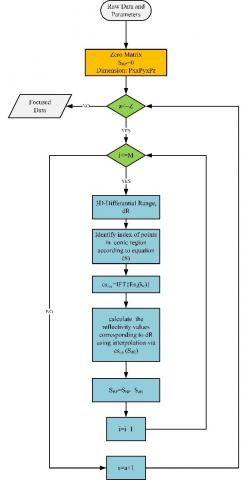
Figure 2. Flow chart for conical 3D-BPA
The expression of the target reflectivity function can be defined as follows:
$\rho(\mathrm{x}, \mathrm{y}, \mathrm{z})=\int_{-z / 2}^{z / 2} \int_0^{+\infty} \int_0^{+\infty} \mathrm{Es}_a\left(\mathrm{k}_{\mathrm{r}}\right) \mathrm{e}^{\mathrm{i} \mathrm{k}_{\mathrm{r}} \mathrm{R}_{\mathrm{p}}} \mathrm{dxdy} \mathrm{dz}$ (4)
If the above equation is written for cylindrical coordinates, it becomes as follows:
$\rho(x, y, z)=\int_{-z / 2}^{+z / 2} \int_{-\pi}^{+\pi} \int_0^{\infty} E s_a\left(k_r\right) e^{i k_r R_p} k_{\mathrm{r}} d k_{\mathrm{r}} d \theta d z$ (5)
The inverse Fourier transform of the expression $\mathrm{Es}_a\left(\mathrm{k}_{\mathrm{r}}\right) \mathrm{k}_{\mathrm{r}}$ in the equation can be written as follows:
$\mathrm{q}_{\mathrm{a}}\left(\mathrm{R}_{\mathrm{p}}\right)=\operatorname{IFT}\left\{\mathrm{Es}_a\left(\mathrm{k}_{\mathrm{r}}\right) \mathrm{k}_{\mathrm{r}}\right\}=\int_0^{+\infty} \mathrm{Es}_a\left(\mathrm{k}_{\mathrm{r}}\right) \mathrm{e}^{\mathrm{ik}_{\mathrm{r}} \mathrm{R}_{\mathrm{p}}} \mathrm{k}_{\mathrm{r}} \mathrm{dk}_r$ (6)
The last expression of reflectivity function is written as follow [12, 45]:
$\rho(\mathrm{x}, \mathrm{y}, \mathrm{z})=\int_{-z / 2}^{z / 2} \int_{-\pi}^{+\pi} \mathrm{q}_{\mathrm{a}}\left(\mathrm{R}_{\mathrm{p}}\right) \mathrm{d} \theta \mathrm{dz}$ (7)
Eq. (7) is the final expression of the traditional BPA at the za vertical position of antennas [47].
On the other hand, implementation of proposed 3D-BPA is given in Figure 2. The algorithm can be summarized in the following steps [15]:
(1) The algorithm starts with the introduction of the experimental parameters. A 3D dimensional SBP matrix consisting of zeroes and i=a=1 are defined.
(2) The main stage of the algorithm starts for za.
(3) In the main stage of the algorithm, the range profile is obtained by applying IFT to the signals reflected from the target for θi angle.
(4) DR values corresponding to possible target range Rp are calculated according to the current position of the antenna.
(5) The reflection values corresponding to the DR are determined by interpolation using the range profile.
(6) The obtained reflection values are summed up with the SBP matrix.
(7) i is incremented by 1 and if i is less than M, algorithm continues by going to step 3.
(8) a is incremented by 1 and if a is less than Z, the algorithm continues by going to step 2; otherwise, it is stopped and focused image data is obtained.
In the traditional BPA, the DR is determined for the entire imaging area, and the reflectance values corresponding to all pixel points of the image scene in step 4 are calculated using the range profile as seen in Eq. (7).
Figure 3. Pixel points of image scene
When the DR is determined for all points in imaging scene as shown in Figure 3(a), undesirable echoes may occur in the image. Therefore, in this study, as in Figure 3(b), DR is calculated for the points inside a conical area. In the implementation of algorithm, only the reflection values corresponding to these points are determined by interpolation. In Figure 3(c), possible target points in the imaging area are shown on the y-z plane. In the proposed method, it is necessary to determine the points within the conic region. The angle $\emptyset_{\mathrm{p}}$ between these points and the y-axis can be determined as follows:
$\emptyset_{\mathrm{p}}=\cos ^{-1} \frac{\sqrt{\left(\mathrm{x}_{\mathrm{i}}-\mathrm{x}_p\right)^2+\left(\mathrm{y}_{\mathrm{i}}-\mathrm{y}_p\right)^2}}{\sqrt{\left(\mathrm{x}_{\mathrm{i}}-\mathrm{x}_p\right)^2+\left(\mathrm{y}_{\mathrm{i}}-\mathrm{y}_p\right)^2+\left(\mathrm{z}_{\mathrm{a}}-\mathrm{z}_p\right)^2}}$ (8)
If $\emptyset_p$ is less than the half angle of the cone's vertex $\emptyset_{cone}$, then this point is in the conical region. In this context, Eq. (7) can be expressed as follows:
$\rho(\mathrm{x}, \mathrm{y}, \mathrm{z})=\sum_{p=1}^P \sum_{i=1}^M \mathrm{q}_{\mathrm{a}}\left(\mathrm{R}_{\mathrm{p}, \mathrm{i}}\right)$ (9)
where, P is the last index of points inside conical area.
Since the number of interpolation points in the proposed method is reduced, the elapsed time of the algorithm is reduced. The performances of the proposed algorithm and the traditional BPA are given in the fourth section using simulation and experimental data.
3.2 Evaluation metrics
Two different metrics, integrated side lobe ratio (ISLR) and computational complexity [14, 48] are used to measure the performance of the proposed method for mmW 3D imaging. While ISLR is an indicator of non-target reflections of the focusing algorithm, the computational complexity gives the matrix processing load required for reconstruction. These two metrics are used as an effective comparison parameter for applications where high resolution and fast results are required.
3.2.1 Computational complexity
Traditional BPA and conical BPA are evaluated in terms of the number of interpolated points. In traditional BPA, for an imaging area with pixel numbers Px, Py, and Pz, interpolation is performed for the total Px×Py×Pz points in the interpolation step [47]. However, since the conical BPA uses points in a conic area, the number of interpolation points is decreased. The interpolation points corresponding to some imaging scene dimensions and voxels are given in Table 1. As can be seen from the results, the number of interpolation points decreased between 2 and 10 times depending on the imaging scene dimensions and the number of pixels. As the dimensions of the imaging scene reduce, the interpolation ratio reduces. In this context, as the dimensions of the imaging scene increase, the interpolation ratio increases. Therefore, the proposed algorithm requires less number of interpolation points for large imaging scene.
3.2.2 Integrated side lobe ratio
ISLR is one of the parameters used to evaluate the performance of algorithms. ISLR is obtained by dividing the within -3dB energy by the total of the remaining energy [48]. ISLR is defined as follows:
$I S L R=\frac{\int_{-3 d B} \quad I d x d y}{\int_{-\infty}^{+\infty} I d x d y-\int_{-3 d B} \quad I d x d y}$ (10)
where, $\int_{-3 d B} I d x d y$ and $\int_{-\infty}^{+\infty} I d x d y$ correspond to the energy within the −3 dB width of the main lobe and total energy, respectively.
Table 1. Number of interpolation points of traditional and proposed BP algorithms
|
$\emptyset_{cone}$ |
Voxels |
Imaging Scene Dimensions |
Number of interpolation points |
Ratio Traditional BPA / Proposed BPA |
|
|
Traditional BPA |
Proposed BPA |
||||
|
5 |
100×100x100 |
1 m×1 m× 1 m |
106 |
102905 |
9.71 |
|
10 |
100×100x100 |
1 m×1 m×1 m |
106 |
207414 |
4.82 |
|
5 |
100×100x100 |
0.5 m×0.5 m× 0.5 m |
106 |
180815 |
5.53 |
|
10 |
100×100x100 |
0.5 m×0.5 m× 0.5 m |
106 |
352823 |
2.83 |
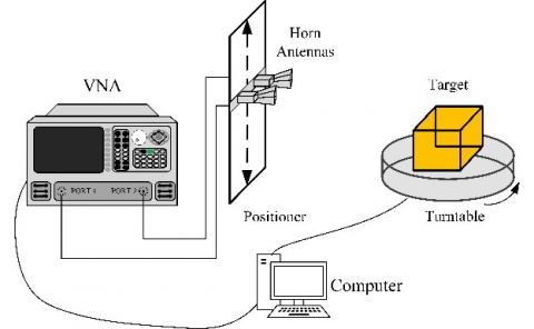
Figure 4. Representation of the experimental system
3.3 Experimental system
The geometry of the experimental system is given in Figure 4. The experiment system consists of EBTRO EAMS turntable, horn antennas operating at frequencies of 26.5-40 GHz, positioner and Keysight 5224A vector network analyser (VNA) and computer. In order to realize the cylindrical scanning geometry, the target is rotated with a turntable at each vertical position of the antennas along the z aperture. Backscattering signals reflected from the target are collected.
4.1 Simulation
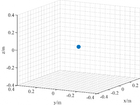
The performance of the proposed method is demonstrated with simulation data. Therefore, an ideal perfect scattering target is used. The target is located at the origin as shown in Figure 5.
Data is collected for the frequency range 26.5 to 40 GHz sampled at 301 points. The cylindrical apertures are a radius of 0.5 m and a height of 0.8 m. The target is scanned for θ=0 to 360 sampled at 721 points for a total of 100 vertical points. The imaging scene dimension is 0.5 m×0.5 m×0.8 m with 128×128×128 voxels.
Figure 5. Coordinates of point scatterer
(a) BPA
(b) proposed BPA
(c) 3D reconstruction result with BP (under -10dB)
(d) 3D reconstruction result with proposed method BP (under -10dB)
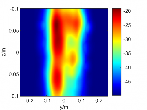
Figure 6. Maximum projection onto yz plane of 3D reconstructed image
The results obtained with the proposed method ($\emptyset_{\text {cone }}=5^{\circ}$) and the traditional BPA are given in Figure 6. When the maximum projection images obtained from 3D images are compared for the -40 dB level, it is seen that the proposed algorithm includes less noise. On the other hand, it is also seen that both algorithms successfully reconstruct 3D images at the -10 dB level.
The performance results of the algorithms are given in Table 2. ISLR of traditional BP is calculated as -13.68 dB, while ISLR of proposed BP is calculated as -8.62 dB. These results show that the proposed algorithm has better side lobe suppression ability. In addition, in the proposed method, the image is obtained using about 88% fewer interpolation points.
Table 2. Performance of algorithms
|
Algorithm |
ISLR (dB) |
# of interpolation points |
|
Traditional BP |
-13.68 |
2097152 |
|
Conical BP |
-8.62 |
233873 |
4.2 Experiment-1 F shaped target
In this experiment, F shaped target with the size of 13 cm x 16 cm is used. The frequency range of the experiment is 26.5-40 GHz with a total number of 301 points. The target is rotated from θ=0 to θ=360 for a total number of 51 vertical points. Vertical and radius aperture lengths of cylindrical scanning geometry are 26 cm and 60 cm, respectively. A scene of experiment 1 is shown in Figure 7.
The 3D images obtained with traditional 3D-BPA and the proposed 3D-BPA and maximum projections onto yz plane is given in Figure 8. It is observed that the image of the target is better focused with proposed method. As can be seen, the image resolution in Figure 8(d) is better than the image in Figure 8(c). While the F shape is not fully formed in Figure 8(c), it is clearly seen in Figure 8(d). In addition, when the reflections in the area of images outside F shape are visually compared in both images, it is clearly seen that a much cleaner background in the reconstructed image is obtained using the proposed method. In this section, the performance of the method is demonstrated using a simple F shaped target. The result of the proposed algorithm is given using a more complex target in the second application.
Figure 7. A scene of first experiment
(a) Traditional BPA
(b) BPA. Maximum projection of 3D images onto yz plane
(c) Traditional BPA
(d) BPA ($\emptyset_{\text {cone }}=$=5º)
Figure 8. Reconstructed 3D image
4.3 Experiment-2 concealed gun
In this experiment, the algorithm is tested under more difficult conditions after a successful result is obtained in the first measurement. Since the plastic mannequin is used, high backscattering signals are reflected from the mannequin. After the system shown in Figure 9(a) is constituted, a 100% cotton t-shirt is put on the mannequin as in Figure 9(b). The measurements are carried out in the anechoic chamber. The frequency range of the experiment is 26.5-40 GHz with a total of 301 points. The target is rotated by 360 degrees with a number of 1144 sample points. Whereas the vertical aperture is 60 cm with a 0.5 cm interval, the radius aperture length is 60 cm.
Figure 9. Scenes of second experiment
(a) Traditional BPA
(b) BPA
Figure 10. Reconstructed 2D image
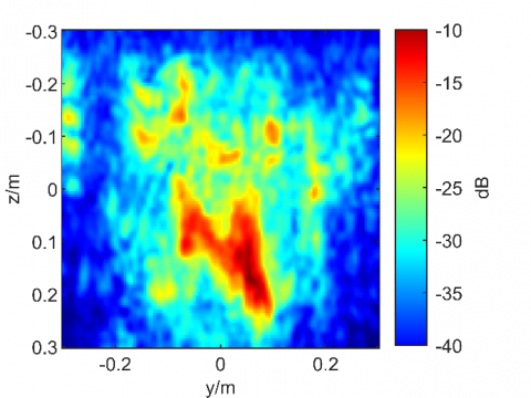
(a) Traditional BPA
(b) BPA
Figure 11. Reconstructed 3D images
2D images obtained from the 3D image, both traditional and conical BPA are given in Figure 10. When Figure 10a is examined, it is not fully understood what the target is in the image obtained with conventional BPA. However, as seen in the image obtained with conical BPA ($\emptyset_{\text {cone }}=5^{\circ}$), it is clearly observed that there is a weapon in the target area.
3D images are given in Figure 11 coloured according to the dynamical range. As seen from the figures, imaging the weapon with the proposed method is more successful than conventional BPA under challenging conditions.
In this study, conical BPA, which uses points inside the conical region in the interpolation step, is proposed for 3D mmW imaging. Therefore, the number of interpolation points and the elapsed time of the algorithm decreased. In addition, ISLR is reduced by the proposed method. The performance of the algorithm is demonstrated by one simulation and two experimental implementations. Cylindrical scanning in simulation and real experiments is carried out at 26.5-40 GHz frequencies. A point scattering target is used in the simulation study. The image of the target is obtained with traditional and conical BPA. The proposed method in terms of ISLR and computational complexity is better than traditional BP. In real experiments, S21 data reflected from the targets are collected along to radius and vertical aperture. The obtained raw data are focused to reconstruct images of the targets using traditional BP and the proposed conical BPA. In the proposed method, while the number of interpolation points decreased, it is observed that the image of targets improved. The results show that it can provide more useful images for applications such as automatic target recognition.
|
x |
X-axis of cartesian coordinate |
|
y |
Y-axis of cartesian coordinate |
|
z |
Z- axis of cartesian coordinate |
|
kr |
two-way propagation constant |
|
P |
total pixel number |
|
Px |
Pixel number of image at x |
|
Py |
Pixel number of image at y |
|
Pz |
Pixel number of image at z |
|
R |
distance from antenna to target |
|
R0 |
distance from antenna to imaging center |
|
Greek symbols |
|
|
δ |
direct delta function |
|
θ |
angle between antenna and x axis |
|
ρ |
reflectiviy function of target |
|
$\emptyset_{\text {p }}$ |
angle between possible target and antenna |
|
$\emptyset_{\text {cone }}$ |
half angle of cone |
|
Subscripts |
|
|
a |
the index of the antenna at the z position |
|
i |
index of θ |
|
p |
index of possible target |
[1] Wang, M., Wei, S., Zhou, Z., Shi, J., Zhang, X. (2022). Efficient ADMM framework based on functional measurement model for mmW 3-D SAR imaging. IEEE Transactions on Geoscience and Remote Sensing, 60: 1-17. https://doi.org/10.1109/TGRS.2022.3165541
[2] Yang, X., Wei, Z., Wang, N., Song, B., Gao, X. (2020). A novel deformable body partition model for MMW suspicious object detection and dynamic tracking. Signal Processing, 174: 107627. https://doi.org/10.1016/j.sigpro.2020.107627
[3] Singh, S., Singh, M. (2003). Explosives detection systems (EDS) for aviation security. Signal Processing, 83(1): 31-55. https://doi.org/10.1016/S0165-1684(02)00391-2
[4] Cheng, B., Cui, Z., Lu, B., Qin, Y., Liu, Q., Chen, P., He, Y., Jiang, J., He, X., Deng, X., Zhang, J., Zhu, L. (2018). 340-GHz 3-D imaging radar with 4Tx-16Rx MIMO array. IEEE Transactions on Terahertz Science and Technology, 8(5): 509-519. https://doi.org/10.1109/TTHZ.2018.2853551
[5] Sheen, D.M., McMakin, D.L., Hall, T.E. (2001). Three-dimensional millimeter-wave imaging for concealed weapon detection. IEEE Transactions on Microwave Theory and Techniques, 49(9): 1581-1592. https://doi.org/10.1109/22.942570
[6] Mirbeik-Sabzevari, A., Oppelaar, E., Ashinoff, R., Tavassolian, N. (2019). High-contrast, low-cost, 3-D visualization of skin cancer using ultra-high-resolution millimeter-wave imaging. IEEE Transactions on Medical Imaging, 38(9): 2188-2197. https://doi.org/10.1109/TMI.2019.2902600
[7] González-Partida, J.T., Almorox-Gonzalez, P., Burgos-García, M., Dorta-Naranjo, B.P., Alonso, J.I. (2008). Through-the-wall surveillance with millimeter-wave LFMCW radars. IEEE Transactions on Geoscience and Remote Sensing, 47(6): 1796-1805. https://doi.org/10.1109/TGRS.2008.2007738
[8] Zhuge, X., Yarovoy, A. G., Savelyev, T., Ligthart, L. (2010). Modified Kirchhoff migration for UWB MIMO array-based radar imaging. IEEE Transactions on Geoscience and Remote Sensing, 48(6): 2692-2703. https://doi.org/10.1109/TGRS.2010.2040747
[9] Wang, G., Qi, F., Liu, Z., Liu, C., Xing, C., Ning, W. (2020). Comparison between back projection algorithm and range migration algorithm in terahertz imaging. IEEE Access, 8: 18772-18777. https://doi.org/10.1109/ACCESS.2020.2968085
[10] Tan, K., Wu, S., Liu, X., Fang, G. (2018). Omega-K algorithm for near-field 3-D image reconstruction based on planar SIMO/MIMO array. IEEE Transactions on Geoscience and Remote Sensing, 57(4): 2381-2394. https://doi.org/10.1109/TGRS.2018.2872918
[11] Li, M., Yue, X., Ding, F., Ning, B., Wang, J., Zhang, N., Luo, J., Huang, L., Wang, Y., Wang, Z. (2022). Focused lunar imaging experiment using the back projection algorithm based on Sanya incoherent scatter radar. Remote Sensing, 14(9): 2048. https://doi.org/10.3390/rs14092048
[12] Yigit, E., Demirci, S., Ozdemir, C., Tekbas, M. (2013). Short-range ground-based synthetic aperture radar imaging: Performance comparison between frequency-wavenumber migration and back-projection algorithms. Journal of Applied Remote Sensing, 7(1): 073483. https://doi.org/10.1117/1.JRS.7.073483
[13] Zeng, G.L. (2012). A filtered backprojection algorithm with characteristics of the iterative Landweber algorithm. Medical Physics, 39(2): 603-607. https://doi.org/10.1118/1.3673956
[14] Özdemir, C., Demirci, Ş., Yiğit, E., Yilmaz, B. (2014). A review on migration methods in B-scan ground penetrating radar imaging. Mathematical Problems in Engineering, 2014: 280738. https://doi.org/10.1155/2014/280738
[15] Demirci, S., Cetinkaya, H., Yigit, E., Ozdemir, C., Vertiy, A. (2012). A study on millimeter-wave imaging of concealed objects: Application using back-projection algorithm. Progress in Electromagnetics Research, 128: 457-477. http://doi.org/10.2528/pier12050210
[16] Gao, J., Deng, B., Qin, Y., Wang, H., Li, X. (2018). An efficient algorithm for MIMO cylindrical millimeter-wave holographic 3-D imaging. IEEE Transactions on Microwave Theory and Techniques, 66(11): 5065-5074. https://doi.org/10.1109/TMTT.2018.2859269
[17] Nan, Y., Huang, X., Guo, Y.J. (2022). 3-D millimeter-wave helical imaging. IEEE Transactions on Microwave Theory and Techniques, 70(4): 2499-2511. https://doi.org/10.1109/TMTT.2022.3151698
[18] Sheen, D.M., McMakin, D.L., Hall, T.E. (2007). Near field imaging at microwave and millimeter wave frequencies. In 2007 IEEE/MTT-S International Microwave Symposium, pp. 1693-1696. https://doi.org/10.1109/MWSYM.2007.380033
[19] Gao, J., Qin, Y., Deng, B., Wang, H., Li, X. (2017). A novel method for 3-D millimeter-wave holographic reconstruction based on frequency interferometry techniques. IEEE Transactions on Microwave Theory and Techniques, 66(3): 1579-1596. https://doi.org/10.1109/TMTT.2017.2772862
[20] Cafforio, C., Prati, C., Rocca, F. (1991). SAR data focusing using seismic migration techniques. IEEE Transactions on Aerospace and Electronic Systems, 27(2): 194-207. https://doi.org/10.1109/7.78293
[21] Zhu, R., Zhou, J., Jiang, G., Fu, Q. (2017). Range migration algorithm for near-field MIMO-SAR imaging. IEEE Geoscience and Remote Sensing Letters, 14(12): 2280-2284. https://doi.org/10.1109/LGRS.2017.2761838
[22] Zhuge, X., Yarovoy, A.G. (2012). Three-dimensional near-field MIMO array imaging using range migration techniques. IEEE Transactions on Image Processing, 21(6): 3026-3033. https://doi.org/10.1109/TIP.2012.2188036
[23] Tan, K., Wu, S., Liu, X., Fang, G. (2018). A modified omega-K algorithm for near-field MIMO array-based 3-D reconstruction. IEEE Geoscience and Remote Sensing Letters, 15(10): 1555-1559. https://doi.org/10.1109/LGRS.2018.2847304
[24] Lopez-Sanchez, J.M., Fortuny-Guasch, J. (2000). 3-D radar imaging using range migration techniques. IEEE Transactions on Antennas and Propagation, 48(5): 728-737. https://doi.org/10.1109/8.855491
[25] Yiğit, E. (2014). Compressed sensing for millimeter-wave ground based SAR/ISAR imaging. Journal of Infrared, Millimeter, and Terahertz Waves, 35(11): 932-948. https://doi.org/10.1007/s10762-014-0094-8
[26] Yigit, E., Kayabaşı, A., Toktaş, A., Sabancı, K., Tekbaş, M., Duysak, H. (2017). Millimetre wave isar imaging technique based on sparse aperture data collection. In 2017 5th International Symposium on Electrical and Electronics Engineering (ISEEE), pp. 1-4. https://doi.org/10.1109/ISEEE.2017.8170663
[27] Wei, S., Zhou, Z., Wang, M., Zhang, H., Shi, J., Zhang, X., Fan, L. (2022). Learning-based split unfolding framework for 3-D Mmw radar sparse imaging. IEEE Transactions on Geoscience and Remote Sensing. https://doi.org/10.1109/TGRS.2022.3181174
[28] Li, S., Zhao, G., Sun, H., Amin, M. (2018). Compressive sensing imaging of 3-D object by a holographic algorithm. IEEE Transactions on Antennas and Propagation, 66(12): 7295-7304. https://doi.org/10.1109/TAP.2018.2869660
[29] Bi, D., Li, X., Xie, X., Xie, Y., Zheng, Y.R. (2021). Compressive sensing operator design and optimization for wideband 3-D millimeter-wave imaging. IEEE Transactions on Microwave Theory and Techniques, 70(1): 542-555. https://doi.org/10.1109/TMTT.2021.3100499
[30] Jing, H., Li, S., Miao, K., Wang, S., Cui, X., Zhao, G., Sun, H. (2022). Enhanced millimeter-wave 3-D imaging via complex-valued fully convolutional neural network. Electronics, 11(1): 147. https://doi.org/10.3390/electronics11010147
[31] Shepp, L.A., Logan, B.F. (1974). The Fourier reconstruction of a head section. IEEE Transactions on Nuclear Science, 21(3): 21-43. https://doi.org/10.1109/TNS.1974.6499235
[32] Scudder, H.J. (1978). Introduction to computer aided tomography. Proceedings of the IEEE, 66(6): 628-637. https://doi.org/10.1109/PROC.1978.10990
[33] Munson, D.C., O'Brien, J.D., Jenkins, W.K. (1983). A tomographic formulation of spotlight-mode synthetic aperture radar. Proceedings of the IEEE, 71(8): 917-925. https://doi.org/10.1109/PROC.1983.12698
[34] Cao, Y., Guo, S., Jiang, S., Zhou, X., Wang, X., Luo, Y., Yu, Z., Zhang, Z., Deng, Y. (2022). Parallel optimisation and implementation of a real-time back projection (BP) algorithm for SAR based on FPGA. Sensors, 22(6): 2292. https://doi.org/10.3390/s22062292
[35] Basu, S., Bresler, Y. (2000). O (N/sup 2/log/sub 2/N) filtered backprojection reconstruction algorithm for tomography. IEEE Transactions on Image Processing, 9(10): 1760-1773. https://doi.org/10.1109/83.869187
[36] Yegulalp, A.F. (1999). Fast backprojection algorithm for synthetic aperture radar. In Proceedings of the 1999 IEEE Radar Conference. Radar into the Next Millennium (Cat. No. 99CH36249), pp. 60-65. https://doi.org/10.1109/NRC.1999.767270
[37] Shao, Y.F., Wang, R., Deng, Y.K., Liu, Y., Chen, R., Liu, G., Loffeld, O. (2013). Fast backprojection algorithm for bistatic SAR imaging. IEEE Geoscience and Remote Sensing Letters, 10(5): 1080-1084. https://doi.org/10.1109/LGRS.2012.2230243
[38] Wahl, D.E., Yocky, D.A., Jakowatz Jr, C.V. (2008). An implementation of a fast backprojection image formation algorithm for spotlight-mode SAR. In Algorithms for Synthetic Aperture Radar Imagery XV, 6970: 95-105. https://doi.org/10.1117/12.779401
[39] Yigit, E., Demirci, S., Unal, A., Ozdemir, C., Vertiy, A. (2012). Millimeter-wave ground-based synthetic aperture radar imaging for foreign object debris detection: experimental studies at short ranges. Journal of Infrared, Millimeter, and Terahertz Waves, 33(12): 1227-1238. https://doi.org/10.1007/s10762-012-9938-2
[40] YİĞİT, E., Özkaya, U., Öztürk, Ş. (2020). Enhancement of near field GB-SAR image quality using beamwidth filter. Avrupa Bilim ve Teknoloji Dergisi, 480-487. https://doi.org/10.31590/ejosat.820286
[41] Ozdemir, C., Demirci, S., Yigit, E. (2008). Practical algorithms to focus B-scan GPR images: Theory and application to real data. Progress in Electromagnetics Research B, 6: 109-122.
[42] Demirci, S., Yigit, E., Eskidemir, I.H., Ozdemir, C. (2012). Ground penetrating radar imaging of water leaks from buried pipes based on back-projection method. Ndt & E International, 47: 35-42. https://doi.org/10.1016/j.ndteint.2011.12.008
[43] Liu, C., Antypenko, R., Sushko, I., Zakharchenko, O., Wang, J. (2021). Marine distributed radar signal identification and classification based on deep learning. Traitement du Signal, 38(5): 1541-1548. https://doi.org/10.18280/ts.380531
[44] Duysak, H., Ozkaya, U., Yigit, E. (2021). Determination of the amount of grain in silos with deep learning methods based on radar spectrogram data. IEEE Transactions on Instrumentation and Measurement, 70: 1-10. https://doi.org/10.1109/TIM.2021.3085939
[45] Rostami, P., Zamani, H., Fakharzadeh, M., Amini, A., Marvasti, F. (2022). A deep learning approach for reconstruction in millimeter-wave imaging systems. IEEE Transactions on Antennas and Propagation, 1-1. https://doi.org/10.1109/TAP.2022.3210690
[46] Zhou, Z., Wei, S., Zhang, H., Shen, R., Wang, M., Shi, J., Zhang, X. (2022). SAF-3DNet: Unsupervised AMP-inspired network for 3-D MMW SAR imaging and autofocusing. IEEE Transactions on Geoscience and Remote Sensing, 60: 1-15. https://doi.org/10.1109/TGRS.2022.3205628
[47] Gao, J., Deng, B., Qin, Y., Wang, H., Li, X. (2018). An efficient algorithm for MIMO cylindrical millimeter-wave holographic 3-D imaging. IEEE Transactions on Microwave Theory and Techniques, 66(11): 5065-5074. https://doi.org/10.1109/TMTT.2018.2859269
[48] Martinez, A., Marchand, J.L. (1993). SAR image quality assessment. Revista de Teledeteccion, 2: 12-18.