Ning Chen* | Shaopeng Wu | Yupeng Chen | Zhanghua Wang | Ziqian Zhang
© 2022 IIETA. This article is published by IIETA and is licensed under the CC BY 4.0 license (http://creativecommons.org/licenses/by/4.0/).
OPEN ACCESS
In response to the problem that the previous pose detection systems are not effective under conditions such as severe occlusion or uneven illumination, this paper focuses on the multimodal information fusion pose estimation problem. The main work is to design a multimodal data fusion pose estimation algorithm for the problem of pose estimation in complex scenes such as low-texture targets and poor lighting conditions. The network takes images and point clouds as input and extracts local color and spatial features of the target object using the improved DenseNet and PointNet++ networks, which are combined with a microscopic bit-pose iterative network to achieve end-to-end bit-pose estimation. Excellent detection accuracy was obtained on two benchmark datasets of LineMOD (97.8%) and YCB-Video (95.3%) for pose estimation. The algorithm is able to obtain accurate poses of target objects from complex scenes, providing accurate, real-time and robust relative poses for object tracking in motion and wave compensation.
multimodal fusion, DenseNet, PointNet++, pose estimation
In the process of parallel supply at sea, due to the action of wind, waves, currents and other environmental factors, the ship will produce movement in six degrees of freedom: heave, sway, surge, pitch, roll and yaw [1, 2], In high sea state, the hydrodynamic interference between the two ships will also produce more violent coupling motion than that of a single ship, which is very likely to cause collision between the lifting cargo and the hull, seriously affecting the safety and efficiency of marine supply operations [3]. Therefore, the development of wave compensation function of the sea supply operations equipment, is to enhance the urgent realistic needs of distant sea escort and ocean combat capabilities.
During the operation of the actual wave compensation system, the position detection system detects the six degrees of freedom movement of the ship under the action of waves in real time, and the control system calculates the change of relative positions of the two ships based on the feedback position data, and servo-controls the movement of the lifting robot arm in space to ensure that the instantaneous relative distance between the lifting cargo and the target position is always the same, so as to achieve the purpose of wave compensation [4, 5]. It can be seen that the real-time detection of the six degrees of freedom attitude change of the ship is a prerequisite for the accurate motion control of the wave compensation device, and plays a decisive role in enhancing the active wave compensation technology.
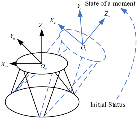
Six-degree-of-freedom stages are widely used in manufacturing assembly [6], wave compensation [7], aerospace [8] and other fields because of their high stiffness, high accuracy, fast response, high load-bearing capacity and relatively easy control. The schematic diagram of the six-degree-of-freedom platform posture detection problem is shown in Figure 1. The six-degree-of-freedom platform consists of six electric actuators, six Hooke hinges on the top and bottom, and two platforms on the top and bottom. The lower platform is a fixed platform, which is fixed on the ground to support the whole system, and the upper platform is a dynamic platform, which can complete the movement of the upper platform in six degrees of freedom in space by controlling the telescopic movement of six electric actuators. The posture of the dynamic platform is an important parameter reflecting the six degrees of freedom platform, which is an important reference value for realizing the closed-loop real-time control of the six degrees of freedom platform, analyzing the dynamic performance of the end-effector, optimizing the design scheme, and analyzing the causes of failure, etc. [9].
Figure 1. Schematic diagram of the six-degree-of-freedom platform posture detection problem
Renaud et al. [10] used a monocular camera to detect the marker points on the branch chain and the moving platform of the H4 parallel mechanism to infer the positional position of the end of the mechanism. Using this method requires the acquisition of more than two images of the branch chain and the acquisition of image depth information, and the movement of the mechanism causes errors in the positioning points during image acquisition, resulting in reduced detection accuracy. Andreff et al. [11] achieved visual servo control of a parallel robot by binocularly photographing the image changes of each branch chain, and it is difficult to achieve tracking and obstacle avoidance of the end-effector because the measurement object is the mechanism branch chain rather than the end-effector. Bellakehal et al. [12] used a visual inspection device to measure the posture of a moving platform and implemented visual servoing based on it, but there are still major limitations in using this method for posture measurement because the measurement object is set to the mechanism support chain.
Vision inspection technology was developed rapidly in the 1990s, and vision-based six-degree-of-freedom platform attitude measurement has gradually become a scientific hotspot. Zhang [13] uses a joint spatio-temporal segmentation algorithm to extract the motion target and describe the six-degree-of-freedom platform poses using three points that are not co-linear on the moving platform. Chen et al. [14] used Harris feature extraction algorithm to track the end-effector of the parallel mechanism and effectively detected the complex motion of the parallel robot in multiple directions and spaces. Zhou and others [15] positioned the center point of the moving platform by image processing technology to achieve the positional measurement of the 3-PRR parallel platform. Gao and Zhang [16] used the Harris-SIFT algorithm to match the features of the acquired moving platform images, and used the RANSAC algorithm to improve the matching accuracy and speed. Cui [17] detected the feature points on the marker plate by binocular camera and solved the position of the moving platform in polar coordinate system. Ren [18] uses a monocular camera to detect rectangular markers pasted on a moving platform and matches the positions of four feature points in the image by the PnP algorithm to achieve the estimation of the position of the parallel robot. Zhao et al. [19] performed 3D reconstruction of the spatial points to obtain the end poses of the parallel mechanism by detecting the four marker points pasted on the moving platform and performing stereo matching. Yang [20] used a coordinate feedback-based corner point detection algorithm and a double-sorted stereo matching algorithm to detect the parallel mechanism poses. Gao and Han [21] matches the actuator end with an improved PROSAC algorithm to solve the problem of degraded positional measurement accuracy due to interference factors such as light and noise.
Traditional bit-pose estimation algorithms generate global features directly from color and depth images, which are prone to undetectable or reduced detection accuracy in the face of complex scenes such as object occlusion and uneven illumination. In this paper, we propose a multimodal data fusion algorithm for pose estimation. The network uses images and point clouds as input, abstracts color and geometric features using a heterogeneous feature extraction network and fuses them, and achieves end-to-end pose estimation by combining a microscopic pose iterative network to achieve an efficient balance between detection accuracy and computational efficiency.
In this section, we present related work and report on the differences of our proposed approach.
2.1 Network framework
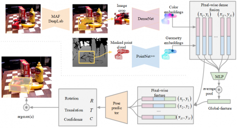
The overall framework of the multimodal information fusion for bit pose estimation algorithm is shown in Figure 2, which includes two stages: multimodal feature fusion and target bit pose prediction. In the first stage, color and geometric features are extracted from both image and point cloud modal data using two heterogeneous networks, respectively, and then fused pixel-by-pixel in the neural network. In the second stage, the initial poses are estimated from the fused features, and then the initial poses are iteratively refined to obtain more accurate poses by means of cyclic learning.
Figure 2. Overall framework of the pose estimation algorithm
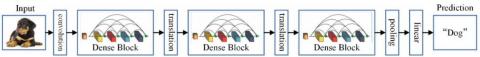
Figure 3. The overall framework of DenseNet
2.2 Network structure improvement
In the actual bit pose estimation process, due to the existence of object occlusion or inaccurate semantic segmentation, the acquired global features may contain a large amount of noise interference from the background or non-target objects, which will lead to a decrease in detection accuracy if fused blindly. In addition, using RGB-D data as input can well solve the problem of uneven lighting, but the disorder of point cloud data makes it difficult to extract geometric features. Therefore, in this paper, based on DenseFusion [22], two heterogeneous networks, improved DenseNet and PointNet++ [23], are used to extract color features and geometric features, respectively, and finally pixel-level feature fusion is performed based on convolutional neural networks.
2.2.1 Color feature extraction
The color feature extraction uses the improved DenseNet network as the color feature extraction backbone network to map the color image of H×W×3 to the geometric space of H×W×d, which makes a close correspondence between the 3D point features and the image features. The overall framework of the DnesnNet network is shown in Figure 3, which focuses on the improvement of the bottleneck and transition layers of the network.
Figure 4. Comparison of bottleneck layer improvements
(1) Bottleneck improvement
As shown in Figure 4(a), the DenseNet network first uses 1×1 convolution to compress the channels to 4k, and then extracts the features by 3×3 convolution. Its densely connected approach leads to the fact that the number of output channels is much larger than the number of input channels after several bottleneck layers of superposition processing, which increases the computational overhead of the intermediate layers. As shown in Figure 4(b), the number of model parameters is reduced by adjusting the number of intermediate channels to be no higher than the number of input channels according to the number of input channels Cin and k. As shown in Figure 4(b), the number of intermediate layer channels is adjusted according to the number of input channels Cin and k not higher than the number of input channels as a way to reduce the number of model parameters. In addition, a new branch consisting of two 3×3 convolutions is added in the bottleneck layer to obtain feature maps with different perceptual fields, taking into account targets of different scales. Finally, the feature maps are densely connected by stitching them together on the channels to ensure the same size and number of channels inside the Block.
(2) Transition layer improvement
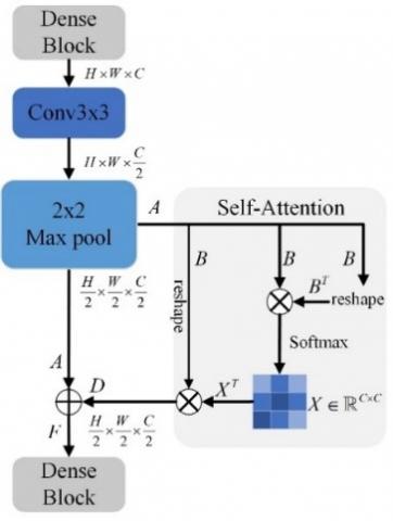
Deep neural networks perceive only through convolutional kernels, which are difficult to capture local contextual information, and this global perception capability is necessary for the network to understand the high-level semantic information of images. For this reason, a self-attention mechanism is introduced at the end of each transition layer, which adaptively learns the weights assigned to each feature channel based on the captured pixel features, enhancing the important channels and suppressing the unimportant ones, giving a huge boost to the deep neural network.
Figure 5. Transition layer improvement measures
As shown in Figure 5, for a given input feature, the feature map $B \in \mathbb{R}^{C \times N}$ and $B^T \in \mathbb{R}^{N \times C}$ is obtained after reconstruction, B and BT are multiplied and input to the softmax layer to obtain the feature map $X \in \mathbb{R}^{c \times c}$. The influence weight of the i-th channel on the j-th channel is:
$x_{j i}=\frac{\exp \left(A_i \cdot A_j\right)}{\sum_{i=1}^N \exp \left(A_i \cdot A_j\right)}$ (1)
In addition, the XT and B matrices are multiplied and the result is reconstructed into $D \in \mathbb{R}^{C \times H \times W}$. The feature map D is then summed element by element with A:
$F_j=\sum_{i=1}^c\left(x_{j i} A_i\right)+A_i$ (2)
The final feature map $F \in \mathbb{R}^{C \times H \times W}$ with feature weighting for all channels is obtained.
2.2.2 Point cloud feature extraction
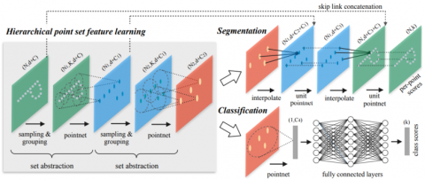
A point cloud is a collection of discrete points in space, which is characterized by disorder, correlation and spatial transformation invariance. By doing feature mapping from low-dimensional to high-dimensional for each point through PointNet network, and then max-pooling all the high-dimensional features can get the global features, but completely ignore the local features between the point pairs [24]. To solve this problem, this paper uses the PointNet++ network [23] shown in Figure 6 as a point cloud feature extraction backbone to obtain richer local geometric features.
PointNet++ borrows the design concept of CNN multilayer perceptron and adopts the coding-decoding structure as the main framework of the network. In the feature encoding network, the point cloud-level feature extraction is mainly realized through a multi-level downsampling structure, in which key points are extracted to construct locally significant feature regions and fully express the point cloud features of local regions. In the feature decoding network, the current feature map is fused with the underlying feature map using the operation of reverse interpolation and jump connection, and the local and global features are recovered by up-sampling step by step, thus completing the point-to-point feature recovery.
2.2.3 Dense feature fusion
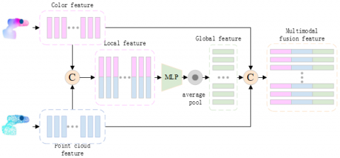
After the above work on improving DenseNet [25] and PointNet++ [23], color features are extracted from images and point clouds along with geometric features. The mainstream approach is to generate global features from segmented regions and deep features, however, when there is mis-segmentation or occlusion, the wrong features may lead to degradation of the bit-pose estimation performance. Therefore, this paper adopts a local pixel-level feature fusion method to reduce the effects of occlusion and illumination on the network, and the specific flow of dense fusion is shown in Figure 7.
Firstly, the geometric and color features of each pixel point are stitched together in the channel dimension to obtain locally fused features. Secondly, the locally fused features are fed into a multilayer perceptron to achieve information integration and global averaging pooling is used to reduce the effect of point cloud disorder, resulting in a global feature vector with richer information content. Finally, the global feature vector is stitched to the back of the local feature vector to obtain a multimodal fusion feature vector with aggregated contextual information.
2.2.4 Pose regression refinement
The pose regression refinement includes a pose regression module, which is used to estimate the initial pose from the fused feature vector, and an iterative refinement of the initial pose.
(1) Pose regression module
After the above operation each fused feature contains three parts: color features, geometric features and global features, and then the fused features are fed into the pose prediction network. As shown in Figure 8, the bit-pose regression module consists of three parts: the rotational vector regression network and the translational vector regression network, as well as the confidence regression network, which are all composed of 3×3 convolution and ReLU activation functions. Each pixel feature input to the network predicts a pose, and eventually a set of predicted poses is obtained, and then the best pose in this set is selected as the initial pose by the confidence regression network.
(2) Iterative refinement module
Most of the positional estimation networks use iterative closest point algorithm (ICP) for positional refinement, which can obtain high positional detection accuracy, but ignores the impact on the real-time performance of the detection algorithm. In this paper, an iterative refinement module based on neural networks is used instead of the traditional way of offline post-processing methods to correct the error of the initial estimated poses in an iterative manner, which can be implemented jointly with the overall network to provide an end-to-end workflow for fast and robust correction of the final pose-estimation results.
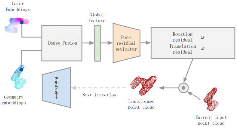
As shown in Figure 9, the positional refinement network is an iterative refinement of the initial estimated poses, i.e., predicting the amount of correction from the last positional estimate. Specifically, in each iteration, the bit pose residual estimator takes the initial bit pose predicted in the previous frame as input, rotates and transforms the point cloud input in the current frame, and inputs it into the current frame. The remaining residual poses are predicted based on the previously estimated poses, and the potential more accurate poses are obtained by iteration. After K iterations, the final positional estimate is obtained as the connection of each iteration estimate:
$\hat{p}=\left[R_K \mid t_K\right] \cdot\left[R_{K-1} \mid t_{K-1}\right] \cdots \cdot\left[R_0 \mid t_0\right]$ (3)
The positional refinement network can be trained jointly with the main network, but the noise of the positional estimation out of the training is too large to learn something meaningful, so the training of the iterative refinement network starts when the loss value is below a set threshold. The positional refinement network can be trained jointly with the main network, but the noise of the positional estimation out of the training is too large to learn something meaningful, so the training of the iterative refinement network starts when the loss value is below a set threshold.
In this section, the details of model training are introduced from three aspects: the measured dataset, the model loss function and the setting of the training strategy.
3.1 Evaluation dataset
In this paper, the evaluation of this paper's method is carried out on two 6D object pose estimation benchmark datasets, LineMOD [26] and YCB-Video [27].
(1) LineMOD datasets
The LineMOD dataset contains 13 videos of low-texture objects against cluttered backgrounds, from which 1214 key frames are selected as the training set and 1335 key frames as the test set, with each frame labeled with only one real 6D pose label of the target object.
(2) YCB-Video datasets
The YCB-Video dataset contains 21 videos of textured objects in indoor scenes, from which 5,000 keyframes are selected as the training set and 1,000 keyframes as the test set. In addition the dataset provides synthetic rendered images to enhance the training set.
3.2 Model loss function
Suppose the translation prediction vector of the ith feature element is $\hat{t}_i$. If the rotation matrix $\hat{R}_i$ obtained from the prediction is combined with the translation vector $\hat{t}_i$, the predicted label between the camera and the target object can be obtained as $\hat{p}_i=\left[\hat{R}_i \mid \hat{t}_i\right]$. Similarly, the true label can be known as $p_i=\left[R_i \mid t_i\right]$. If xj denotes the jth point of M key points randomly selected from the real label of the object, the visual positional estimation loss function can be defined as the distance between the real label of the object and the corresponding point on the predicted label.
$L_i^p=\frac{1}{M} \sum_j\left\|\left(R x_j+t\right)-\left(\hat{R}_i x_j+\hat{t}_i\right)\right\|$ (4)
If the target is a symmetric object, the above loss function will cause the learning target to be blurred and multiple cases of correct poses may be obtained using Eq. (4), when the distance between the predicted label and the nearest point on the true pose-label can be minimized to estimate the loss function will change to Eq. (5).
$L_i^p=\frac{1}{M} \sum_j \min _{0<k<M}\left\|\left(R x_j+t\right)-\left(\hat{R}_i x_k+\hat{t}_i\right)\right\|$ (5)
In addition, based on the contextual information of each key point it can be determined which bit pose is the best hypothesis, and the final loss function is defined as Eq. (6).
$L=\frac{1}{N}\left(L_i^p c_i-w \ln c_i\right)$ (6)
In Eq. (6), N is the number of dense pixel features randomly drawn from the real model p, and w is a balanced hyperparameter. A low confidence level causes a low positional estimation loss and leads to a high penalty in the second term, and conversely the highest confidence level predicted positional is used as the final output.
3.3 Experimental training strategy
In this paper, we adopt the same training strategy as DenseFusion [22], using real labels during training and split labels during testing. The experimental hardware includes Intel(R) Core(TM) i7-9750H CPU @ 2.60GHz, NVIDIA GeForce RTX 2080×2. The experimental operating system is Ubuntu 18.04, and the software used is CUDA10.0, Pytorch1.2.0. The model training epoch is set to 100, and the initial learning rate is 0.001. The initial learning rate is 0.001, and when the loss value decreases to 0.018, the iterative refinement of the model is started, and the number of iterations is set to 2.
This section first presents the experimental measurement dataset, experimental implementation details, and evaluation metrics. Next, the effectiveness of the proposed modules is analyzed through an ablation study. Then the proposed method is compared with the existing techniques and the effectiveness of the proposed method is verified by quantitatively analyzing the model segmentation performance based on the experimental results. Finally the visualization results of the proposed method on two datasets are analyzed qualitatively in order to get a more intuitive feeling.
4.1 Evaluation indicators
To comprehensively evaluate the proposed approach, the average closest point distance (ADD-S) and the model average distance (ADD) are used as quantitative metrics in this paper.
For non-symmetric objects, the average closest point distance (ADD-S) is used for evaluation. As shown in Eq. (7), the average distance between two models of predicted poses and ground truth poses was calculated. When the distance is less than 10% of the model diameter, the predicted poses are considered to be correct.
$A D D-S=\frac{1}{M} \sum_j \min _{0<k<M}\left\|\left(R x_j+t\right)-\left(\hat{R}_i x_j+\hat{t}_i\right)\right\|$ (7)
For symmetric objects, the average distance (ADD) of model points is used for evaluation, as shown in Eq. (8). The distance is calculated using the nearest point, and the nearest distance can be calculated by the fast search algorithm KNN (KNearest Neighbor).
$A D D=\frac{1}{M} \sum_j\left\|\left(R x_j+t\right)-\left(\hat{R}_i x_j+\hat{t}_i\right)\right\|$ (8)
4.2 Model ablation experiments
In order to verify the effect of bitwise iterative refinement and to obtain the optimal number of iterations, ablation experiments with 0-4 bitwise iterative refinements were designed in this paper, and the experimental results are shown in Table 1.
The pose refinement module can significantly improve the accuracy of the final pose prediction and achieve the original purpose of the network design. As the results in the table show, two iterations of refinement are finally chosen in this paper after each prediction of the initial pose, while satisfying the real-time requirements of pose estimation.
Table 1. Pose estimation results of ablation experiments
|
Evaluation dataset |
Accuracy |
||||
|
0th |
1th |
2th |
3th |
4th |
|
|
LineMOD [26] |
94.6 |
96.2 |
97.8 |
97.6 |
96.7 |
|
YCB-Viedo [27] |
92.1 |
95.1 |
95.3 |
95.0 |
95.1 |
4.3 Model performance comparison
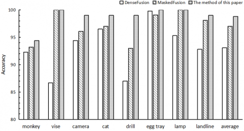
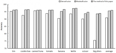
In order to better evaluate the performance of the multimodal information fusion pose estimation algorithm, this paper compares with two methods, DenseFusion [22]and MaskedFusion [28], on two pose estimation benchmark datasets, LineMOD [26] and YCB-Viedo [27], and the results are shown in Figures 10 and 11.
Figure 10. Comparison with the same type of method on the LineMOD dataset
Figure 11. Comparison with the same type of methods on the YCB-Viedo dataset
The method in this paper achieves a significant improvement over the same type of positional estimation network because the model uses both image and point cloud modal data, and the interaction between the extracted color and geometric features strengthens the mapping relationship between the features and the positional information, making the positional estimation algorithm more efficient.
4.4 Comparison of detection effects
In this section, the proposed network is tested on LineMOD and self-built container datasets, and the final output of the network is rotation vectors with translation vectors. In order to express the effect of the positional detection more intuitively, the results of the network prediction are projected onto a two-dimensional image for qualitative analysis of the model performance, and the visualization results are shown in Figure 10.
(1) LineMOD Datasets
Figure 12 shows the visualization of the experimental results in the LineMOD dataset. From the figure, it can be seen that the algorithm can well weaken the influence of environmental factors on the positional estimation results, and it is also applicable to a variety of situations such as poor lighting conditions and low-texture targets, which demonstrates the reliability of the positional estimation algorithm in this paper.
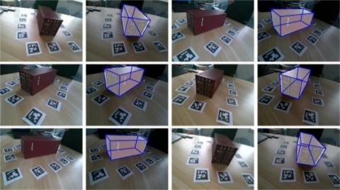
(2) Self-built Container Datasets
Figure 13 shows the visualization of the experimental results on the container dataset. From the figure, it can be seen that the positional estimation results fit the containers better under different lighting conditions, which shows the reliability of the positional estimation algorithm in this paper.
Figure 12. Visualization of experimental results on LineMOD dataset
Figure 13. Visualization of experimental results on container dataset
In this paper, we propose a multimodal information fusion approach for pose estimation for six degrees of freedom pose detection problem in complex scenes. First, the network takes RGB-Point heterogeneous data as input, and extracts dense color features of the input image by a modified DenseNet network and spatial geometric features of the input point cloud using a PointNet++ network. Then, the extracted color features are embedded into the spatial features to achieve pixel-level feature fusion, and the target coarse poses are estimated based on the fused features. Finally, using a differentiable bit-pose iterative network, the rough bit-pose estimate of the previous frame is iterated cyclically as the initial bit-pose to fit a more accurate bit-pose and achieve end-to-end bit-pose estimation. The proposed method obtains excellent positional detection results on two positional estimation benchmark datasets, LineMOD (97.8%) and YCB-Video (95.3%), which can better cope with the effects of severe occlusion and changes in lighting conditions, and initially meets the requirements of a wave-compensated positional detection system.
This project was supported by the Fujian Province Natural Science Foundation (Grant No.: 2021J01851) and the Jimei University National Natural Science Foundation Incubation Program (Grant No.: ZP2020045).
[1] Bai, Y., Hu, Y. (2016). Discussion on the development trends of wave compensation technology of offshore alongside replenishment. Naval Architecture and Ocean Engineering, 32(5): 1-4. https://doi.org/10.14056/j.cnki.naoe.2016.05.001
[2] Liu, Y., Zhong, L. (2020). Research on key technologies of ship wave compensation. Ship Science and Technology, 42(10): 7-9.
[3] Zhao, L., Wu, S. (2020). Wave compensation and optimal design of 6-DOF Industrial Robo. Ship Science and Technology, 42(22): 19-21. https://doi.org/10.3404/j.issn.1672-7649.2020.11A.007
[4] Li, R. (2019). Research on ship motion simulation and mechanical arm lifting motion compensation control. Changchun, China: Jilin University, 2019.
[5] Gu, X., Xu, J., Liu, Z. (2021). Design and control method of the wave compensation mechanism of ship's relief supply device. Ship Engineering, 43(11): 133-138.
[6] Huang, S. (2018). Research and application of key assembly technology of carrier aircraft landing gear. Harbin, China: Harbin Institute of Technology, 2018.
[7] Xu, X. (2021). Stereo pose Realtime tracking and detection based on deep learning. Amoy, China: JiMei University, 2021.
[8] Xu, W. (2018). Design and research of large gesture flight simulator based on hybrid mechanism. Beijing, China: Beijing Jiaotong University, 2018.
[9] Li, Y.B., Zheng, H., Xu, M.R., Luo, Y.Q., Sun, P. (2019). Multi-target parameters of performance optimization for 5-PSS/UPU parallel mechanism. Journal of Zhejiang University (Engineering Science), 53(4): 654-663.
[10] Renaud, P., Andreff, N., Lavest, J.M., Dhome, M. (2006). Simplifying the kinematic calibration of parallel mechanisms using vision-based metrology. IEEE Transactions on robotics, 22(1): 12-22. https://doi.org/10.1109/TRO.2005.861482
[11] Andreff, N., Dallej, T., Martinet, P. (2007). Image-based visual servoing of a gough—Stewart parallel manipulator using leg observations. The International Journal of Robotics Research, 26(7): 677-687. https://doi.org/10.1177/0278364907080426
[12] Bellakehal, S., Andreff, N., Mezouar, Y., Tadjine, M. (2011). Vision/force control of parallel robots. Mechanism and Machine Theory, 46(10): 1376-1395. https://doi.org/10.1016/j.mechmachtheory.2011.05.010
[13] Zhang, S., Ding, Y., Hao, K. (2008). Measurement of position and orientation of 6-DOF large load test platform based onstereo vision. Application Research of Computers, 25(6): 1744-1746.
[14] Chen, J., Ding, Y., Hao, K. (2009). Vision pose measurement for parallel robot based on object tracking. Computer Engineering, 35(18): 200-202+205. https://doi.org/10.3969/j.issn.1000-3428.2009.18.070
[15] Zhou, L. (2013). Research on Key Technology of Precision Position based on Machine Vision for a 3-PRR parallel manipulator Driven by Linear Ultrasonic Motors. Nanking, China: Nanjing University of Aeronautics and Astronautics, 2013.
[16] Gao, G., Zhang, S. (2016). Pose detection for a novel parallel mechanism based on binocular vision. Measurement & Control Technology, 35(11): 14-17+21. https://doi.org/10.3969/j.issn.1000-8829.2016.11.004
[17] Cui, W. (2016). Research on Measuring Technology of Six Degree of Freedom for Waving Compensation Based on Binocular Vision. Changsha, China: National University of Defense Technology, 2016.
[18] Ren, S. (2017). Research of the Parallel robot’s Kinematic Calibration and Pose Tracking based on vision. Harbin, China: Harbin Engineering University, 2017.
[19] Zhao, J., Liu, Z., Huang, J., Chen, G.Q., Dai, J. (2018). The method to measure the terminal position and pose of 3-PRS parallel mechanism based on binocular vcision system. Manufacturing Technology & Machine Tool, 2018(1): 101-106. https://doi.org/10.19287/j.cnki.1005-2402.2018.01.020
[20] Yang, L. (2019). Study on Corner Detection and Pose Detection of Parallel Mechanism Moving Platform Based on Binocular Vision. Qinhuangdao, China: Yanshan University, 2019.
[21] Gao, G., Han, Y. (2020). Pose detection for visual blindness of parallel robot. Computer Measurement & Control, 28(9): 100-105. https://doi.org/10.16526/j.cnki.11-4762/tp.2020.09.020
[22] Wang, C., Xu, D., Zhu, Y., Martín-Martín, R., Lu, C., Li, F.F., Savarese, S. (2019). Densefusion: 6d object pose estimation by iterative dense fusion. In Proceedings of the IEEE/CVF Conference on Computer Vision and Pattern Recognition, Long Beach, CA, USA, pp. 3343-3352. https://doi.org/10.1109/CVPR.2019.00346
[23] Chen, Y., Liu, G., Xu, Y., Pan, P., Xing, Y. (2021). PointNet++ network architecture with individual point level and global features on centroid for ALS point cloud classification. Remote Sensing, 13(3): 472. https://doi.org/10.3390/rs13030472
[24] Qi, C.R., Su, H., Mo, K., Guibas, L.J. (2017). Pointnet: Deep learning on point sets for 3d classification and segmentation. In Proceedings of the IEEE Conference on Computer Vision and Pattern Recognition, Honolulu, HI, USA, pp. 652-660. https://doi.org/10.1109/CVPR.2017.16
[25] Chen, Y., Chen, N., Wang, Q. (2021). Densely connected image classification algorithm combining with self-attention. In International Workshop of Advanced Manufacturing and Automation, Singapore, pp. 332-340. https://doi.org/10.1007/978-981-19-0572-8_42
[26] Hinterstoisser, S., Holzer, S., Cagniart, C., Ilic, S., Konolige, K., Navab, N., Lepetit, V. (2011). Multimodal templates for real-time detection of texture-less objects in heavily cluttered scenes. In 2011 International Conference on Computer Vision, Barcelona, Spain, pp. 858-865. https://doi.org/10.1109/ICCV.2011.6126326
[27] Calli, B., Walsman, A., Singh, A., Srinivasa, S., Abbeel, P., Dollar, A.M. (2015). Benchmarking in manipulation research: The YCB object and model set and benchmarking protocols. arXiv preprint arXiv:1502.03143. https://doi.org/10.48550/arXiv.1502.03143
[28] Pereira, N., Alexandre, L.A. (2020). MaskedFusion: Mask-based 6D object pose estimation. In 2020 19th IEEE International Conference on Machine Learning and Applications (ICMLA), Miami, FL, USA, pp. 71-78. https://doi.org/10.1109/ICMLA51294.2020.00021