Illakiya Thayumanasamy | Karthik Ramamurthy*
© 2022 IIETA. This article is published by IIETA and is licensed under the CC BY 4.0 license (http://creativecommons.org/licenses/by/4.0/).
OPEN ACCESS
Alzheimer's disease (AD) is an irreversible and degenerative brain condition that gradually damages memory and thinking abilities. Despite being incurable, AD causes significant pain and financial hardship to patients and their families. However, medications are most effective when administered early in the course of the disease and early diagnosis is crucial in the treatment of AD to restrict its progression. There are several approaches proposed for computer-assisted AD diagnosis that involve structural and functional imaging modalities, such as sMRI, fMRI, DTI, and PET. Machine learning and deep learning techniques have facilitated the development of novel models for diagnostic accuracy in AD. This research compares the performance of several machine learning and deep convolutional architectures to detect AD from MCI. It is essential to find the effective baseline model for classifying AD, hence all the pre-trained models are evaluated with benchmark dataset. Experimental observations indicate that the DenseNet-169 performed best out of different state-of-the-art architectures, with an average accuracy of 82.2%.
Alzheimer’s disease, machine learning, deep learning, classification, magnetic resonance imaging
AD is a neurological problem that cannot be reversed and causes gradual memory loss and cognitive decline. According to reports, there are 26.6 million AD patients globally, and of those, 56% are in the early stages. According to WHO report, there will be 152 million people affected by AD worldwide in 2050. AD commonly affect the neurons in the entorhinal cortex and hippocampus regions of the brain that are responsible for the memory and thinking ability of the person. Furthermore, it damages the cerebral cortex that controls language and behavioural patterns [1]. The primary sign of AD is loss of memory. The symptoms of early Alzheimer's include difficulty recalling previous interactions or events. Memory deficits develop as the condition worsens, and other symptoms appear [2]. Memory difficulties and other cognitive abnormalities due to AD may temporarily be eased by current Alzheimer's treatments. The behavioural symptoms of AD may occasionally be managed with the use of additional drugs, such as antidepressants. There are currently no effective treatments for the complete cure while existing AD medicines can only ease symptoms or slow their progression. The prevention and intervention of AD's progression, therefore, depends on the diagnosis of the early or prodromal stage. Mild Cognitive Impairment (MCI) is typically regarded as the initial stage of AD and is considered as the right stage for early intervention. According to research, persons with MCI are at an increased risk of getting Alzheimer's disease [3]. The cause of AD is most likely a combination of genetics, lifestyle, and environmental factors [4].
Neuroimaging technologies have been extensively used in recent years for the diagnosis of AD and MCI. The understanding of structural and functional brain alterations associated with AD has been greatly aided by the use of Magnetic Resonance Imaging (MRI), an imaging modality that creates comprehensive 3D anatomical images of the brain [5]. Especially, the structural MRI (sMRI) provides detailed information about the anatomical structure of the brain, making it useful for detecting and measuring the atrophy patterns in AD [6]. To treat the disease successfully, it must be detected as early as possible, even before symptoms develop. The need for reliable diagnostic methods is therefore important for preventing or slowing the disease. Numerous machine learning algorithms have been used recently to evaluate the sMRI images to identify biomarkers and understand the progression of the disease. Due to the lack of a thorough understanding of the subtle pathological changes in the brain, it is still difficult for physicians to characterise AD features from MRIs. For this reason, deep learning techniques have the potential to be far more effective than techniques that rely on manually generated features [7]. Convolutional neural networks (CNNs), a type of deep learning framework, have often been used in image classification and computer vision. In contrast to machine learning, it has the advantage of requiring fewer pre-processing of images and using raw images to automatically integrate optimal features without manual feature selection. Furthermore, CNN algorithms have proven to be successful in diagnosing AD using neuroimages [8].
This paper is structured as follows: Section 2 explores the related literature. The materials and techniques used are described in Section 3. The results of the experiment and performance analysis are presented in Section 4. The conclusion is provided in Section 5.
The application of deep learning and machine learning for the identification of AD has made significant advancements in recent years. The main categories for the classification of AD: the approaches based on machine learning and the methods based on deep learning are reviewed in this section.
2.1 Machine learning methods
Traditional machine learning methods use handcrafted features to understand the trends associated with detection of AD. K-Nearest Neighbours (KNN), Naïve Bayes, and Support Vector Machines (SVM) are some of the machine learning methods that are used to classify AD. For instance, Zhang et al. used SVM with different kernels to make an accurate prediction of AD [9]. PCA was used for eigen brain generation. Similarly, Sudharsan and Thailambal used PCA for feature selection, IVM, RELM and SVM for classification [10]. Lodha et al. analysed several ML-based algorithms such as k-means, decision trees and neural networks [11]. From the experiment, it was inferred that neural networks gave better accuracy than other ML methods. Further, Uysal and Ozturk analysed the various ML algorithms such as linear regression, KNN, SVM, decision tree, random forest and gaussian naïve Bayes [12]. The left and right hippocampal volume, age, and gender are used for the classification. A similar approach was proposed by Mirzai and Adeli, where supervised learning methods such as SVM, random forest and unsupervised methods such as k-means, hierarchical, fuzzy, spectral, density-based clustering, and Bayesian techniques were analysed [13]. A resampling approach was applied by Cabrera-Leon et al. to alleviate class imbalance, and a counter propagation network was compared with an ensemble of non-neural networks for classifying AD [14]. Though Machine learning approaches are used in the majority of AD diagnosis strategies, it suffers from a few limitations like requiring domain knowledge for proper feature selection, and human intervention in segmentation etc., Deep learning techniques, on the other hand, have been used by researchers to improve performance in AD classification using neuroimaging data. The primary reason is that the deep learning methods provide better accuracy on diverse data sets [15-20], so they are most suitable for AD detection using MRI.
2.2 Deep learning methods
In several studies, deep learning approaches were used to classify AD. The pre-trained models are a kind of CNN architecture that is used in transfer learning where the learnt parameters from one model are utilised as input parameters in another model to produce accurate results. The similarity between input and target data maximizes the effectiveness of the classification task. Transfer learning has been used extensively in the field of AD classification. AlexNet, VGG16, ResNet, and other deep neural network models have been employed successfully for AD classification.
Maqsood et al. performed transfer learning by using AlexNet architecture for the classification of AD [21]. The fully connected layers are replaced by a softmax layer, fully connected layer and output classification layer. A similar modification of AlexNet architecture was performed by Ghazal and Issa [22]. The AlexNet layers are customized according to Alzheimer’s dataset and could be able to perform multiclass classification [22]. To improve the accuracy of the diagnostic system, Tanveer et al. used 3D MRI from ADNI and a small local dataset. DL agnostic ensemble strategies were implemented for the detection of AD [23]. A slice-wise averaging and slice-wise ensemble max voting was used in this work. The VGG-16 network was used as a feature extractor in similar work by Jain et al. [24]. Input MRI images were pre-processed with freesurfer and classified using the freesurfer tool. With the use of the ResNet model, Puente-Castro et al. attempted to automatically detect AD from sagittal MRI [25]. Furthermore, other details, such as the age and sex of the patients, were fed into the system. A modified version of the ResNet architecture was incorporated by Oktavian et al. for training [26]. The default activation function ReLU was replaced by the mish activation function.
A recent study by Liu et al. used AlexNet and GoogleLeNet for TL [27]. Optimum results were achieved by replacing traditional convolution with depth-wise separable convolution (DSC). An analysis of AlexNet, GoogleNet, VGGNet-16, VGGNet-19, MobileNetv2, Squeezenet, ResNet-18,50,101, Inception-ResNet V2, Inception V3, DenseNet and Spiking neural networks (SNN) for feature extraction was conducted by Ashraf et al. [28]. The DenseNet model reportedly outperformed other CNN models in terms of performance.
All the above approaches include one or more machine learning or deep learning techniques for the classification of AD. Though few methods employed benchmark dataset for evaluation, most of the works were developed with limited and restricted datasets obtained from clinical sources. Hence, there exist a vital need to analyse the performance of all methods cumulatively with a benchmark dataset. This will help us to identify the optimal backbone architecture for further architectural enhancement to obtain better accuracy.
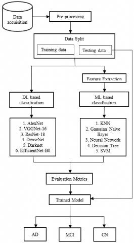
This section discusses the dataset description, block diagram, and methodologies used in this work. Figure 1 presents the overall system architecture. An extensive study of state-of-the-art machine learning models and deep architectures for detecting AD has been conducted in this work. Machine learning algorithms like Decision tree, Gaussian Naïve Bayesian, KNN, SVM and Neural Networks were analysed. AlexNet, VGGNet-16, ResNet-18, ResNet-34, ResNet-50, ResNet-152, DenseNet-121, DenseNet-169, DenseNet-201, Darknet, EfficientNet-B0 have been examined using various performance criteria.
3.1 Dataset acquisition
The dataset was downloaded from the public ADNI database, which can be accessed at http://www.loni.ucla.edu/ADNI. In 2003, ADNI was developed by the National Institute on Aging, the National Institute of Biomedical Imaging and Bioengineering, the Food and Drug Administration (FDA), pharmaceutical firms, and non-profit organizations. The primary objective of ADNI is to evaluate the sequence MRI, PET, other biomarkers, clinical, and neuropsychological tests may be integrated to detect the progression of the disease and early AD [29, 30]. A total of 585 subjects including 175 AD, 256 MCI and 154 NC subjects are used in this work.
3.2 Pre-processing
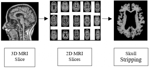
Pre-processing steps are required to prepare the input data to produce proper classification results. The sMRI images that are in. nii (Neuroimaging Informatics Technology Initiative) format are pre-processed. Initially, the 3D MRI voxels are transformed into 2D slices. Figure 2 depicts the pre-processing tasks done in this work.
Figure 1. Overview of the proposed experimentation
Further, skull striping was performed to remove non-brain tissue and unnecessary sections of a scanned image. Morphological structuring was used to eliminate the scalp, skull, and dura from the sMRI.
Figure 2. Pre-processing of sMRI
3.3 Data augmentation
Image data augmentation is a technique for intentionally increasing the size of a dataset by modifying images in the dataset. In order to enhance the performance and generalizability of the model, data augmentation was used commonly. Additionally, they were applied to address the class imbalance problem. The images were initially scaled to a dimension of 128 x 128. Random geometric modifications such as flipping and rotation were used to expand the dataset. The random rotation parameter range is 0° to 90°, and the probability of random horizontal and vertical flips is set to 50% each. The augmented brain MRI images are shown in Figure 3. The Torchvision library was used to perform all modifications.
Figure 3. Augmented brain MRI
3.4 Machine learning methods
The features of the pre-processed images are extracted and given as an input to the classifier. This section explains the various features extracted and the ML algorithms used in this analysis.
3.4.1 Feature extraction
Classification of images can be done efficiently by using feature extraction techniques. It is an approach for reducing a big input data set into important features. The first, second, and higher order statistical features are extracted. A total of 4 first-order features, 19 second-order features and 7 higher-order features are used for further process. The texture of the region is described using statistical vectors based on the features described above.
(1) First-order features
The intensity distributions within the image region are described by first-order statistics. The first 4 moments of the probability density function are the first-order statistical features [31]. Arithmetic mean is defined as the first moment of a probability density function defining the gray level intensity in a Region of Interest (ROI). Generally, it is not accurate in distinguishing a region of interest from its surrounding areas. The second moment is the standard deviation that calculates the range or dispersion from the mean value. The skewness of a matrix is the third moment that quantifies the asymmetry of the value distribution around the Mean value. Skewness in a matrix indicates the difference in illumination between texture pixels (texels) and average illumination. Texels with a positive skew are darker than average, whereas those with a negative skew are lighter. The uniformity in gray level distribution can be determined by the fourth moment of a matrix, known as the kurtosis.
(2) Second-order features
The Gray-Level Co-Occurrence Matrix (GLCM) is a well-known second-order statistical method proposed by Haralick et al. used to extract textural data [32]. To distinguish the textural uniqueness of the ROI, GLCM characteristics are retrieved. It provides information about the impact of grey-level intensity varies on distance and direction. The 19 GLCM features described by Haralick [32] provide textural information that could be used to distinguish regions of interest. The contrast, correlation, homogeneity, entropy etc., are some of the commonly used GLCM features.
(3) Higher-order features
A Gray-Level Run-Length Matrix (GLRLM) is a higher-order statistical feature that is used to differentiate a set of images from another one [33]. A gray level run can be quantified by using GLRLM, which measures the length of consecutive pixels with the same gray level value. The (i,j)th element of a grey level run length matrix P(i,j) represents the number of runs with length j and grey level I that appear in the image (ROI) across the angle θ. Galloway described the typical GLRLM characteristics [34]. Gray Level Non-Uniformity (GLNU), Short Run Emphasis (SRE), Run Length Non-Uniformity (RLNU), Long Run Emphasis (LRE), Run Percentage (RP), Low Gray Level Run Emphasis (LGLRE), and High Gray Level Run Emphasis (HGLRE) are the features used in this work.
3.4.2 ML based classification
In this experiment, five different machine learning models were used to classify AD. These models include the Decision tree, Gaussian Naïve Bayesian, KNN, SVM and Neural Networks.
(1) KNN
KNN is a non-parametric supervised learning which presumes that related objects are located nearby. Classification is determined by a majority of neighbour votes, and the object is assigned to the class that has the most k nearest neighbours. Due to the fact that the algorithm does not learn directly from the training set, it is sometimes referred to as a lazy learner algorithm.
(2) Gaussian naive bayes
A Naive Bayes classifier uses the Bayes theorem to construct probabilistic classifications. Every attribute variable is treated independently in the Naive Bayes classification. This classifier can be efficiently used in challenging real-world scenarios. This algorithm is particularly advantageous as it requires a few training data, which is crucial for classification. In a Gaussian Naive Bayes algorithm, it is common to assume that the continuous values corresponding to each class are distributed according to the Gaussian distribution. A mean and standard deviation are calculated for each class after splitting the training data.
(3) Neural networks
Neural Networks consist of three layers: an input layer, one or more hidden layers, and an output layer. Each neuron or node in the layer is linked to another and has a distinct weight and threshold. A node gets activated and starts transmitting data to the successive layer, if its output is greater than the threshold value for that node. The weights help determine the importance of each given variable, with larger ones contributing more strongly to the outcome than smaller ones. The goal of artificial neural networks is to solve complex problems more accurately.
(4) Decision tree
A decision tree is a supervised ML algorithm that replicates the way humans make decisions by using a set of rules. The idea behind decision tree is to repeatedly partition the dataset until all the data points that belong to each class are isolated by using the dataset features to produce yes/no questions. Internal nodes and leaf nodes are terms used to describe intermediate subsets and leaves, respectively. When features and the target interact significantly, a decision tree is most helpful.
(5) SVM
SVM is a supervised learning technique that is most commonly employed for regression, classification and outliers detection problems. In order to classify n-dimensional space, the SVM method seeks to establish the best line. So that the new data point can then be easily placed into the correct category in the future. Hyperplanes are boundaries that represent the best decisions. Support vectors or decision functions are the closest data points or vectors to the hyperplane, and they affect the hyperplane's position. SVM can be extended to perform non-linear classification jobs where the collection of data cannot be split linearly. The decision function can be specified with different kernel functions like Linear, Polynomial, Gaussian Radial Basis Function etc.
3.5 Deep learning based classification
The objective of this research is to analyse the state-of-the-art architectures for detecting AD effectively. They include Alexnet, EfficientNet-B0, ResNet, VGGNet, DarkNet, and DenseNet.
3.5.1 AlexNet
The performance of AlexNet in 2012 ImageNet LSVRC-2012 Competition showed it to be one of the most popular deep CNN architectures [35, 36]. This architecture has 22 layers and Rectified Linear Unit (ReLU) is used as the activation function. It accepts the input image with a dimension of 256 x 256. It can detect up to 1000 classes with the help of 60 million parameters [37]. During training, resized images were fed into the network and the output layer used a two-way soft-max function.
3.5.2 VGGNet
According to the ILSVRC challenge 2014, VGG-16 was among the top performing architectures. A VGG architecture can be used to classify and learn features from input images that are 224 x 224 pixels [38]. Each layer except the final dense layer used rectified linear unit as its activation function.
3.5.3 ResNet
The use of skip connections is the main characteristic of the ResNet architecture [39]. It accepts the input image with a dimension of 224 x 224. Vanishing gradients are a common issue with deep neural networks as the gradient value suddenly decreases in the back-propagation phase. This has an impact on the convergence of the network. To address this issue, ResNet employs skip connections. These connections will skip specific levels, assisting in the reduction of the vanishing gradient problem.
3.5.4 DenseNet
In a DenseNet, every layer is directly connected with each other using Dense Blocks, which acts as dense connections between layers [40]. It accepts the input image with a dimension of 224 x 224. By concatenating outputs from previous layers, subsequent layers are created. A feature map from each preceding layer is used as an input for each new layer. In the output layer of the model, a softmax layer was used as activation function to train the model.
3.5.5 DarkNet
As part of YOLOv3, Darknet was developed in 2018 and used to extract fundamental features. It combines YOLOv2's basic feature extraction framework with residual network. The model has five blocks, each with two convolution layers of size 1x1 and 3x3, followed by a residual layer [41].
3.5.6 Efficientnet-B0
EfficientNet employs a scaling approach that equally scales all depth/width/resolution dimensions using a compound coefficient [42]. It accepts the input image with a dimension of 224 x 224. In contrast to current practise, which arbitrarily scales these elements, the EfficientNet scaling approach evenly scales network depth, breadth and resolution using a set of parameters. It uses a compound scaling method, which allows easy and principled scaling up of a baseline ConvNet while maintaining model efficiency.
This section discusses the performance of the machine learning models and deep learning models in the experiments conducted for the AD classification.
4.1 Environmental setup
The AWS EC2 instance's Pytorch framework and 16GB NVIDIA T4 GPU were used to implement all image pre-processing operations and train the model. Ubuntu 20.04 operating system, 4 AMD vCPUs, and 32GB RAM are system specifications used for the implementation. AMP CUDA was used to decrease the network's training time without compromising performance. Furthermore, gradient scaling was used during backpropagation to avoid the problem of vanishing gradients. A 80:20 ratio was used to divide the dataset into training and testing groups.
4.2 Hyperparameter tuning
Hyperparameter tuning of pre-trained models was performed using the Grid Search algorithm in the Ray Tune framework. There were two hyperparameters set in the model for the experiment: (1) learning rate of the optimizer and (2) batch size. The learning rate of the optimizer was set between 1e-1 and 1e-5; batch size was either 32 or 64. Optimal tuning was achieved by iterating over the search space of parameter values in the defined range. Pre-trained networks converged optimally with learning rates of 1e-3 and batch size of 32. The number of epochs is fixed as 50.
4.3 Evaluation metrics
The performance of the classification models was analyzed using accuracy, recall, precision, and F1-scores. 5-fold cross-validation was used to further analyse and validate them. An accuracy metric is the percentage of data points predicted correctly. It is calculated by the relation (1).
Accuracy $=\frac{T P+T N}{T P+T N+F P+F N}$ (1)
where, TP signifies the true positive, which was correctly predicted to be positive. TN is a true negative, exactly predicted as negative. False negative (FN) predictions are supposed to be negative. False positive (FP) is erroneously interpreted as positive.
Sensitivity, also known as recall, is a number of positives that are accurately predicted out of all the expected positive values. The recall is computed as shown in relation (2).
Sensitivity $=\frac{T P}{T P+F N}$ (2)
An F1-score measures how well precision and recall balance out in a model. This is calculated according to relation (3).
$F 1-$ score $=\frac{2 * \text { Precision } * \text { Recall }}{\text { Precision }+\text { Recall }}$ (3)
Precision is defined as the proportion of correctly classified positives (True Positive) and incorrectly classified positives (either correctly or incorrectly classified). It is calculated by the relation (4).
Precision $=\frac{T P}{T P+F P}$ (4)
4.4 Performance analysis
The model predictions, analysis, and final results are discussed in this section.
4.4.1 Analysis of ML methods
Based on the performance of the ML models, the accuracy, recall, precision, and F1-score are computed. Table 1 also presents the performance of the models being categorized based on the GLCM, GLRLM and combination of both GLCM and GLRLM features extracted and used in classification.
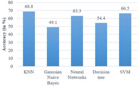
On comparing the results of all models, it is evident that KNN and SVM gave the best overall accuracy compared to other models as shown in Figure 4. It is also inferred that the combination of GLCM and GLRLM features gave good accuracy in all the models used in this work.
Figure 4. Comparison of accuracy in ML models
4.4.2 Analysis of DL methods
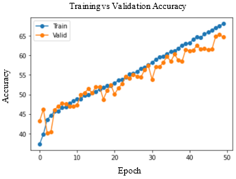
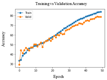
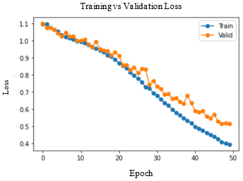
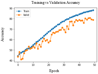
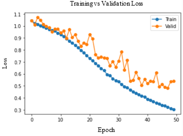
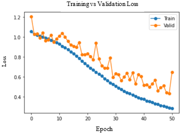
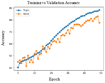
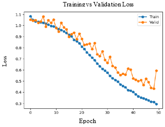
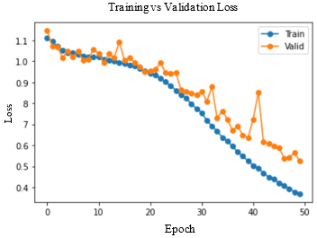
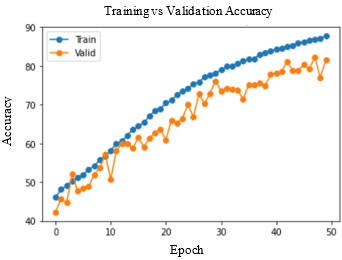
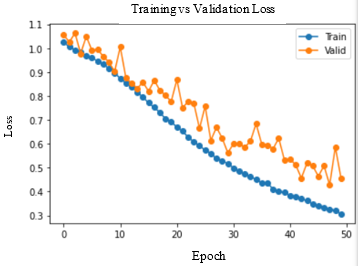
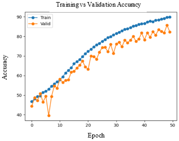
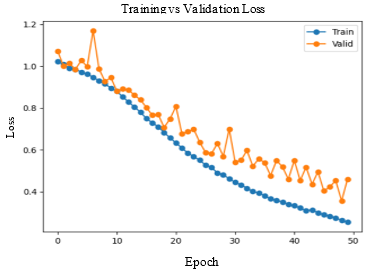
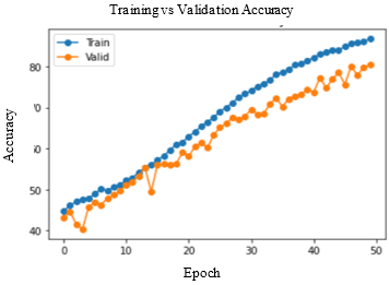
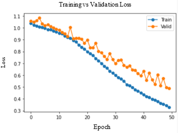
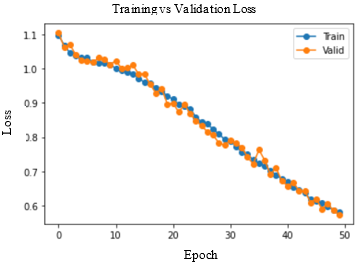
Accuracy and Loss were used to analyse the training performance of different deep learning models. The accuracy of the state-of-art methods is summarized in Table 3. The observations obtained after training each of these models for 50 epochs and their observations are shown in Table 2.
As seen in Figure 5, DenseNet-169 and DenseNet-201 models produced significantly better results for testing sets. Table 4 lists the class-wise evaluation measures, including recall, precision, and F1-score. DenseNet-169 achieved the highest accuracy of 82.2% among the machine learning and deep learning algorithms used in this analysis. DenseNet-201 is the second accurate approach, with an accuracy of 81.6%. Customising the pre-trained models or utilizing the complex CNNs would bring great improvement in performance of the AD diagnostic system.
Figure 5. Comparison of accuracy in state-of-the-art architectures
Table 1. Performance comparison of different ML models
|
Model |
K-nearest neighbour |
Gaussian Naive Bayes |
Neural Networks |
Decision tree |
Support Vector Machines |
||||||||||
|
GLCM |
GLRLM |
Combined features |
GLCM |
GLRLM |
Combined features |
GLCM |
GLRLM |
Combined features |
GLCM |
GLRLM |
Combined features |
GLCM |
GLRLM |
Combined features |
|
|
Accuracy |
62.1 |
52.1 |
68.8 |
46.5 |
46.2 |
49.1 |
55.6 |
50.4 |
63.3 |
48.4 |
47.6 |
54.4 |
59.1 |
54.8 |
66.5 |
|
Precision |
61.6 |
52.3 |
68 |
42 |
41 |
39.2 |
53.6 |
51 |
61.3 |
49 |
48 |
53.3 |
58.3 |
54.3 |
66.6 |
|
Recall |
61 |
52.6 |
68 |
37 |
40.6 |
37.3 |
52 |
50.6 |
60 |
56 |
47.3 |
54.3 |
57.3 |
53.6 |
65 |
|
F1-Score |
61.6 |
51 |
67.3 |
29 |
36.6 |
36.3 |
51 |
51 |
61.6 |
46 |
46.6 |
53.3 |
57 |
53.6 |
66 |
Table 2. Observations of training performance for different DL models
|
Architecture |
Accuracy |
Loss |
|
AlexNet |
||
|
VGGNet-16 |
||
|
ResNet-18 |
||
|
ResNet-34 |
||
|
ResNet-50 |
||
|
ResNet-152 |
||
|
DenseNet-121 |
||
|
DenseNet-169 |
||
|
DenseNet-201 |
||
|
DarkNet |
||
|
EfficientNet-B0 |
Table 3. An analysis of pre-trained architectures based on accuracy
|
S.No |
Model trained |
Number of trainable parameters |
Accuracy (in %) |
|
1 |
AlexNet |
57M |
64.69 |
|
2 |
VGGNet-16 |
134M |
78.82 |
|
3 |
ResNet-18 |
11M |
78.69 |
|
4 |
ResNet-34 |
21M |
76.09 |
|
5 |
ResNet-50 |
23M |
77.6 |
|
5 |
ResNet-152 |
58M |
79.2 |
|
6 |
DenseNet-121 |
6M |
81.51 |
|
7 |
DenseNet-169 |
12M |
82.2 |
|
8 |
DenseNet-201 |
18M |
81.6 |
|
9 |
Darknet |
26M |
80.43 |
|
10 |
EfficientNet-B0 |
4M |
75.01 |
Table 4. Class-wise metrics for the deep learning models trained
|
Model trained |
Precision |
Recall |
F1-Score |
||||||
|
AD |
CN |
MCI |
AD |
CN |
MCI |
AD |
CN |
MCI |
|
|
AlexNet |
62 |
58 |
74 |
73 |
70 |
56 |
74 |
56 |
64 |
|
VGGNet-16 |
78 |
79 |
79 |
77 |
78 |
80 |
79 |
80 |
80 |
|
ResNet-18 |
69 |
83 |
86 |
90 |
74 |
74 |
78 |
78 |
79 |
|
ResNet-34 |
75 |
69 |
83 |
80 |
80 |
72 |
77 |
74 |
77 |
|
ResNet-50 |
78 |
67 |
88 |
79 |
89 |
70 |
79 |
76 |
78 |
|
ResNet-152 |
79 |
77 |
80 |
77 |
78 |
81 |
78 |
77 |
81 |
|
DenseNet-121 |
80 |
77 |
86 |
85 |
83 |
78 |
83 |
80 |
82 |
|
DenseNet-169 |
80 |
81 |
85 |
84 |
80 |
83 |
82 |
80 |
84 |
|
DenseNet-201 |
81 |
75 |
88 |
83 |
90 |
76 |
82 |
82 |
82 |
|
Darknet |
80 |
76 |
84 |
80 |
83 |
79 |
80 |
80 |
81 |
|
EfficientNet-B0 |
75 |
66 |
84 |
73 |
88 |
69 |
74 |
75 |
76 |
The key objective of this research is to evaluate the performance of deep convolutional networks and cutting-edge machine learning models for the classification of AD using MRI images. Machine learning models such as KNN, Gaussian Naïve Bayesian, Decision tree, Neural Networks and SVM were used in the analysis. The state-of-art deep architectures, including AlexNet, VGGNet-16, ResNet-18, ResNet-34, ResNet-50, ResNet-152, DenseNet 121, DenseNet-169, DenseNet-201, Darknet, EfficientNet-B0 were also used for detailed evaluation. Various metrics were used to evaluate the performance of these methods, such as precision, recall, and F1-score. According to the results and analysis, DenseNet-169 outperformed other architectures with an accuracy of 82.2%. The performance of the DL models can still be improved by layer-wise fine-tuning with larger datasets. Other architectural customizations can be done with a backbone model. This will hopefully enable accurate early diagnosis and treatment of AD patients, which will improve their quality of life.
[1] National Institute on Aging. (n.d.). National Institute on Aging. https://www.nia.nih.gov/, accessed on August 16, 2022.
[2] Alzheimer’s disease—Symptoms and causes—Mayo Clinic. (n.d.). https://www.mayoclinic.org/diseases conditions/alzheimers-disease/symptoms-causes/syc-20350447, accessed on August 16, 2022.
[3] Sarraf, S., Desouza, D.D., Anderson, J.A., Saverino, C. (2019). MCADNNet: Recognizing stages of cognitive impairment through efficient convolutional fMRI and MRI neural network topology models. IEEE Access, 7: 155584-155600. https://doi.org/10.1109/ACCESS.2019.2949577
[4] Bhushan, I., Kour, M., Kour, G., Gupta, S., Sharma, S., Yadav, A. (2018). Alzheimer’s disease: Causes & treatment – A review. Annals of Biotechnology, 1(1). https://doi.org/10.33582/2637-4927/1002
[5] Johnson, K.A., Fox, N.C., Sperling, R.A., Klunk, W.E. (2012). Brain imaging in Alzheimer disease. Cold Spring Harbor Perspectives in Medicine, 2(4): a006213.
[6] Liu, M., Li, F., Yan, H., Wang, K., Ma, Y., Shen, L., Xu, M. (2020). A multi-model deep convolutional neural network for automatic hippocampus segmentation and classification in Alzheimer’s disease. NeuroImage, 208: 116459. https://doi.org/10.1016/j.neuroimage.2019.116459
[7] Ge, C., Qu, Q., Gu, I.Y.H., Jakola, A.S. (2019). Multi-stream multi-scale deep convolutional networks for Alzheimer’s disease detection using MR images. Neurocomputing, 350: 60-69. https://doi.org/10.1016/j.neucom.2019.04.023
[8] Feng, W., Halm-Lutterodt, N.V., Tang, H., Mecum, A., Mesregah, M.K., Ma, Y., Li, H., Zhang, F., Wu, Z., Yao, E., Guo, X. (2020). Automated MRI-based deep learning model for detection of Alzheimer’s disease process. International Journal of Neural Systems, 30(6): 2050032. https://doi.org/10.1142/S012906572050032X
[9] Zhang, Y., Dong, Z., Phillips, P., Wang, S., Ji, G., Yang, J., Yuan, T.F. (2015). Detection of subjects and brain regions related to Alzheimer’s disease using 3D MRI scans based on Eigen brain and machine learning. Frontiers in Computational Neuroscience, 9. https://doi.org/10.3389/fncom.2015.00066
[10] Sudharsan, M., Thailambal, G. (2021). Alzheimer’s disease prediction using machine learning techniques and principal component analysis (PCA). Materials Today: Proceedings. https://doi.org/10.1016/j.matpr.2021.03.061
[11] Lodha, P., Talele, A., Degaonkar, K. (2018). Diagnosis of Alzheimer’s Disease Using Machine Learning. 2018 Fourth International Conference on Computing Communication Control and Automation (ICCUBEA), pp. 1-4. https://doi.org/10.1109/ICCUBEA.2018.8697386
[12] Uysal, G., Ozturk, M. (2020). Hippocampal atrophy based Alzheimer’s disease diagnosis via machine learning methods. Journal of Neuroscience Methods, 337: 108669. https://doi.org/10.1016/j.jneumeth.2020.108669
[13] Mirzaei, G., Adeli, H. (2022). Machine learning techniques for diagnosis of Alzheimer disease, mild cognitive disorder, and other types of dementia. Biomedical Signal Processing and Control, 72: 103293. https://doi.org/10.1016/j.bspc.2021.103293
[14] Cabrera-Leon, Y., Baez, P.G., Ruiz-Alzola, J., Suarez-Araujo, C.P. (2018). Classification of mild cognitive impairment stages using machine learning methods. 2018 IEEE 22nd International Conference on Intelligent Engineering Systems (INES), pp. 000067-000072. https://doi.org/10.1109/INES.2018.8523858
[15] Karthik, R., Menaka, R., Hariharan, M., Won, D. (2022). Contour-enhanced attention CNN for CT-based COVID-19 segmentation. Pattern Recognition, 125: 108538. https://doi.org/10.1016/j.patcog.2022.108538
[16] Karthik, R., Vaichole, T.S., Kulkarni, S.K., Yadav, O., Khan, F. (2022). Eff2Net: An efficient channel attention-based convolutional neural network for skin disease classification. Biomedical Signal Processing and Control, 73: 103406. https://doi.org/10.1016/j.bspc.2021.103406
[17] Karthik, R., Radhakrishnan, M., Rajalakshmi, R., Raymann, J. (2021). Delineation of ischemic lesion from brain MRI using attention gated fully convolutional network. Biomedical Engineering Letters, 11(1): 3-13. https://doi.org/10.1007/s13534-020-00178-1
[18] Karthik, R., Menaka, R., Hariharan, M., Won, D. (2022). CT-based severity assessment for COVID-19 using weakly supervised non-local CNN. Applied Soft Computing, 121: 108765. https://doi.org/10.1016/j.asoc.2022.108765
[19] Karthik, R., Menaka, R., Hariharan, M., Won, D. (2021). Ischemic lesion segmentation using ensemble of multi-scale region aligned CNN. Computer Methods and Programs in Biomedicine, 200: 105831. https://doi.org/10.1016/j.cmpb.2020.105831
[20] Radhakrishnan, M., Ramamurthy, K., Choudhury, K.K., Won, D., Manoharan, T.A. (2021). Performance Analysis of Deep Learning Models for Detection of Autism Spectrum Disorder from EEG Signals. Traitement du Signal, 38(3): 853-863. https://doi.org/10.18280/ts.380332
[21] Maqsood, M., Nazir, F., Khan, U., Aadil, F., Jamal, H., Mehmood, I., Song, O.Y. (2019). Transfer learning assisted classification and detection of Alzheimer’s disease stages using 3D MRI scans. Sensors, 19(11): 2645. https://doi.org/10.3390/s19112645
[22] Ghazal, T.M., Issa, G. (2022). Alzheimer disease detection empowered with transfer learning. Computers, Materials & Continua, 70(3): 5005-5019. https://doi.org/10.32604/cmc.2022.020866
[23] Tanveer, M., Rashid, A.H., Ganaie, M.A., Reza, M., Razzak, I., Hua, K.L. (2021). Classification of Alzheimer’s disease using ensemble of deep neural networks trained through transfer learning. IEEE Journal of Biomedical and Health Informatics, 26(4): 1453-1463. https://doi.org/10.1109/JBHI.2021.3083274
[24] Jain, R., Jain, N., Aggarwal, A., Hemanth, D.J. (2019). Convolutional neural network based Alzheimer’s disease classification from magnetic resonance brain images. Cognitive Systems Research, 57: 147-159. https://doi.org/10.1016/j.cogsys.2018.12.015
[25] Puente-Castro, A., Fernandez-Blanco, E., Pazos, A., Munteanu, C.R. (2020). Automatic assessment of Alzheimer’s disease diagnosis based on deep learning techniques. Computers in Biology and Medicine, 120: 103764. https://doi.org/10.1016/j.compbiomed.2020.103764
[26] Oktavian, M.W., Yudistira, N., Ridok, A. (2022). Classification of Alzheimer’s Disease Using the Convolutional Neural Network (CNN) with Transfer Learning and Weighted Loss (arXiv:2207.01584). arXiv. http://arxiv.org/abs/2207.01584.
[27] Liu, L., Zhao, S., Chen, H., Wang, A. (2020). A new machine learning method for identifying Alzheimer’s disease. Simulation Modelling Practice and Theory, 99: 102023. https://doi.org/10.1016/j.simpat.2019.102023
[28] Ashraf, A., Naz, S., Shirazi, S.H., Razzak, I., Parsad, M. (2021). Deep transfer learning for Alzheimer neurological disorder detection. Multimedia Tools and Applications, 80(20): 30117-30142. https://doi.org/10.1007/s11042-020-10331-8.b
[29] Wyman, B.T., Harvey, D.J., Crawford, K., Bernstein, M. A., Carmichael, O., Cole, P.E., Alzheimer's Disease Neuroimaging Initiative. (2013). Standardization of analysis sets for reporting results from ADNI MRI data. Alzheimer's & Dementia, 9(3): 332-337. https://doi.org/10.1016/j.jalz.2012.06.004
[30] Jack Jr, C.R., Bernstein, M.A., Fox, N.C., Thompson, P., Alexander, G., Harvey, D., Weiner, M.W. (2008). The Alzheimer's disease neuroimaging initiative (ADNI): MRI methods. Journal of Magnetic Resonance Imaging: An Official Journal of the International Society for Magnetic Resonance in Medicine, 27(4): 685-691. https://doi.org/10.1002/jmri.21049
[31] Schilling, C. (2012). Analysis of Atrial Electrograms (Vol. 17). KIT Scientific Publishing.
[32] Haralick, R.M. (1979). Statistical and structural approaches to texture. Proceedings of IEEE, 67(5): 786-804. https://doi.org/10.1109/PROC.1979.11328.
[33] Chu, A., Sehgal, C.M., Greenleaf, J.F. (1990). Use of Gray value distribution of run lengths for texture analysis. Pattern Recognition Letters, 11(6): 415-419. https://doi.org/10.1016/0167-8655(90)90112-F
[34] Galloway, M.M. (1975). Texture analysis using Gray level run lengths. Computer Graphics and Image Processing, 4(2): 172-179. https://doi.org/10.1016/S0146-664X(75)80008-6.
[35] Valverde, J.M., Imani, V., Abdollahzadeh, A., De Feo, R., Prakash, M., Ciszek, R., Tohka, J. (2021). Transfer learning in magnetic resonance brain imaging: a systematic review. Journal of Imaging, 7(4): 66. https://doi.org/10.3390/jimaging7040066
[36] Krizhevsky, A., Sutskever, I., Hinton, G.E. (2017). Imagenet classification with deep convolutional neural networks. Communications of the ACM, 60(6): 84-90. https://doi.org/10.1145/3065386
[37] Kumar, L. S., Hariharasitaraman, S., Narayanasamy, K., Thinakaran, K., Mahalakshmi, J., Pandimurugan, V. (2022). AlexNet approach for early stage Alzheimer’s disease detection from MRI brain images. Materials Today: Proceedings, 51: 58-65. https://doi.org/10.1016/j.matpr.2021.04.415
[38] Simonyan, K., Zisserman, A. (2014). Very deep convolutional networks for large-scale image recognition. arXiv preprint arXiv:1409.1556. https://doi.org/10.48550/arXiv.1409.1556
[39] He, K., Zhang, X., Ren, S., Sun, J. (2016). Deep residual learning for image recognition. In Proceedings of the IEEE Conference on Computer Vision and Pattern Recognition, pp. 770-778. https://doi.org/10.48550/arXiv.1512.03385
[40] Huang, G., Liu, Z., Van Der Maaten, L., Weinberger, K.Q. (2017). Densely connected convolutional networks. In Proceedings of the IEEE Conference on Computer Vision and Pattern Recognition, pp. 4700-4708. https://doi.org/10.48550/arXiv.1608.06993
[41] Redmon, J., Farhadi, A. (2018). Yolov3: An incremental improvement. arXiv preprint arXiv:1804.02767. https://doi.org/10.48550/arXiv.1804.02767
[42] Tan, M., Le, Q. (2019). Efficientnet: Rethinking model scaling for convolutional neural networks. In International Conference on Machine Learning, pp. 6105-6114. https://doi.org/10.48550/arXiv.1905.11946