A Road Extraction Method of a High-Resolution Remote Sensing Image Based on Multi-Feature Fusion and the Attention Mechanism

Na Jiang* | Jiyuan Li | Jingyu Yang | Junting Lin | Baopeng Lu
© 2022 IIETA. This article is published by IIETA and is licensed under the CC BY 4.0 license (http://creativecommons.org/licenses/by/4.0/).
OPEN ACCESS
Road extraction from high-resolution remote sensing images has a lot of practical value and significance and has been a research hotspot. Considering that methods based on deep learning and the attention mechanism have achieved good performance in road detection, this paper proposes a deep residual network and an attention mechanism based on the fusion of multiple road features. The encoder–decoder structure of the U-net network with strong multitasking generality is adopted as the basic network. It integrates the spatial multi-scale and multi-channel features of the road to enhance the robustness of feature extraction. Meanwhile, the decoder design based on the attention mechanism further improves the recognition accuracy and effectively curbs the increase in computing cost and time cost. A loss function based on the gradient coordination mechanism is introduced to address the imbalance of road sample data. Finally, experimental verification is carried out on two public road datasets and both qualitative and quantitative comparisons are conducted. Results show that the proposed method is satisfactory and outperforms other methods.
attention mechanism, deep learning, multi-channel feature, remote sensing, road extraction
With the rapid development in space science and technology, the number of high-resolution remote sensing satellites in orbit continues to increase. This has reduced the acquisition cost of high-resolution earth observation image data, and the data acquired are more diverse and comprehensive. Compared with low-resolution remote sensing image data, high-resolution remote sensing image data have more spatial details, providing a large amount of rich data with clear details for remote sensing scientific research [1-3]. With the large amount of high-resolution remote sensing im-age data, the research on remote sensing feature classification and detection, including the research on terrain classification and road detection, has made great progress [4, 5]. Road extraction based on remote sensing images has wide applications, for example, in map update, urban planning, unmanned navigation, disaster relief, and mitigation [6-8].
For road extraction, investigations have been carried out for decades. Zhao et al. [9] proposed the use of PCA to analyze the multi-spectral bands to combine the multi-spectral features with statistical features for road detection. Shi et al. [10] and Miao et al. [11] adopted the adaptive classification method to analyze the multi-spectral features and combined road geometric features to extract non-occluded roads. Que et al. [12], Shanmugam et al. [13], and Mu et al. [14] compared each pixel grayscale feature in remote sensing images with one or more thresholds for road detection and declared that the difference and critical points help determine the optimal threshold. Tan and Zeng realized road extraction and detection by using the edge detection algorithm of the Sobel operator and Canny operator [15, 16]. Cai et al. [17] proposed an improved watershed algorithm to segment the image into individual connected closed regions and select appropriate thresholds to optimize road segmentation. Jin et al. [18] proposed a regional value-added algorithm that continuously merges pixels that can satisfy the judgment conditions and grows iteratively as new seeds. Cheng et al. [19] proposed a method based on texture and geometric features of remote sensing images for road extraction, which is not satisfactory for discontinuous road recognition.
In recent years, deep learning algorithms have made remarkable achievements in the fields of computer vision and artificial intelligence. Cheng et al. [3] proposed a cascaded end-to-end convolutional neural network (Cas Net) to automatically complete road region extraction and road centerline extraction and further used the results for road region detection. This method overcomes the problem of vehicle and tree occlusion. Lu et al. [20] proposed a multi-scale multi-task deep learning framework to automatically complete both road region extraction and midline extraction. In addition, a convolutional neural network method based on edge enhancement was pro-posed [21], which effectively overcomes the influence of tree shadow and vehicle interference in the images.
High-resolution remote sensing images contain a large number of features related to ground objects, and road data account for a small proportion of these features. A model with high feature learning and feature expression capabilities is required to accurately and comprehensively identify and extract road features. Therefore, it is a great challenge to overcome the data imbalance between ground objects to accurately extract road features from high-resolution remote sensing images.
Road information is hierarchical, that is, in high-resolution images of different sizes, the road presents different feature information. It is necessary to carry out feature extraction at different scales and fuse the feature information on different scales to obtain the complete features of the road accurately. Therefore, multi-scale road feature recognition is another major challenge.
In addition, deep learning methods rely on a large number of convolution operations to complete the learning and training of model parameters, which involves a large computing cost. Since convolution is not effective for every computation, many computations are redundant, leading to unnecessary costs and time expenditure. Therefore, how to reduce invalid calculations, saving on calculation costs and shortening training time, is also a key problem of deep-learning-based road recognition methods.
To overcome the above mentioned problem, this paper proposes a novel deep learning network for road extraction from high-resolution remote sensing images—MRAU. The main contributions of this paper are as follows:
A deep-learning-based road extraction method with multi-feature fusion is proposed. Features of different spatial scales and multi-channels are extracted using the atrous space pyramid method and the residual-based compression excitation network, respectively.
A road feature recognition method based on the attention mechanism is proposed. The attention gate network module is designed in the decoding stage to improve the metrics without significantly increasing the redundant calculation and time cost.
A loss function for road recognition based on the gradient coordination mechanism is constructed to solve the unbalanced problems of positive and negative samples as well as the difficult and easy samples of road target datasets.
The rest of this paper is organized as follows: Section 2 details the theoretical prevalence of the proposed method, and Section 3 presents both the implementations of numerical tests and the results. The conclusions are drawn in Section 4.
In this section, the main sections of the MRAU framework for road detection are explained, which are related methods and Multi-scale Residual Attention U-net for Road Detection.
2.1 Review of relative methods
2.1.1 U-net
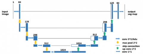
In 2015, Ronneberger et al. [22] proposed the U-net network structure that can obtain higher segmentation accuracy by classifying each pixel of the input image (as shown in Figure 1).
Figure 1. The network structure of U-net
The U-net is simple in structure and is used for image semantic segmentation, with the image under segmentation as input and segmentation results as output. The U-net is mainly composed of three parts: down sampling, up sampling, and skip connection. Down sampling achieves insight and expression of image features, up sampling realizes image restoration, and skip connection preserves and transmits image information of the same size. U-net is a lightweight network with 28 megabits of parameters. Its structure has good adaptability. Similar to the FCN, U-net is often used as the basic skeleton network.
2.1.2 SE-ResNet
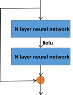
The residual neural network, proposed by He et al. [23] in 2016, is mainly used to solve the problem of network degradation caused by the increasing number of neural network layers. The invented shortcut connection can effectively eliminate the training problem of a deep learning network (as shown in Figure 2).
The residual neural network realizes identity mapping through the shortcut con-nection structure so that the learning of y = H(x) is equivalent to the learning of y = F(x)+x, namely F(x) = H(x) - x, called residuals.
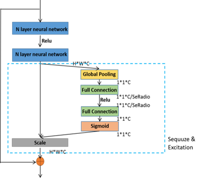
The squeeze-and-excitation network (SEnet), also known as the compression and excitation network, is an image recognition neural network structure proposed by Hu et al. [24] in 2017 and is mainly composed of squeeze operation and excitation operation. For SEnet, first, the interdependence between its input image channels is modeled and then the feature response strength relationship between channels is obtained through global loss function training. As shown in Figure 3, the compression and excitation network is fused with the residual network structure, as described in [24], to form the SE-ResNet network structure.
Figure 2. Original structure of ResNet
Figure 3. The network structure of SE-ResNet
SE-ResNet applies the squeeze-and-excitation module to the residual module: (i) SE-ResNet reduces the feature dimension W of the channel to W/SeRadio, where Se-Radio is the squeeze coefficient, (ii) it is activated by Relu, and (iii) it passes through a fully connected layer. In this way, the complex correlation between channels can be fitted better and the number of parameters and computations can be minimized.
2.1.3 ASPP
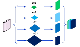
In 2018, Chen et al. [25] proposes the atrous spatial pyramid pooling (ASPP) model, which can increase the receptive field without increasing the number of parameters so that more semantic information of adjacent pixels can be obtained (as shown in Figure 4).
Figure 4. The network structure of ASPP
2.1.4 Attention gates
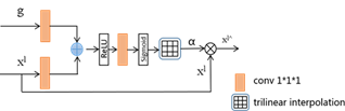
In 2018, Ozan et al. [26] proposed the attention gates model (as shown in Figure 5), which automatically learns the shape and size of the object to be segmented. This is an attention mechanism model and can learn to focus on learning useful salient regions and sup-press the learning of irrelevant background regions during training.
Figure 5. The network structure of attention gate
As shown in Figure 5, α (value 0~1) is the attention coefficient. By multiplying the attention coefficient and the feature map, the value of the irrelevant region in the feature map becomes smaller, while the value of the target region becomes larger. Since the attention gate model has limited parameters, it can achieve feature suppression of irrelevant background regions without a lot of training. At the same time, the attention gate model has good versatility and can be embedded in many convolutional neural network models to improve their performance.
2.1.5 GHM-C loss
Li et al. [27] proposed a coordination mechanism from the perspective of gradient. Balancing the contribution of gradients in the learning process of different samples weakens the gradient accumulation generated by simple samples and outliers to make training more effective and stable.
A common classification loss function is cross-entropy.
$L_{C E}\left(p, p^*\right)= \begin{cases}-\log (p) & p^*=1 \\ -\log (1-p) & p^*=0\end{cases}$ (1)
where, p and p* are the predicted probability and true probability, respectively. Let x be the output of the model. Then, the gradient of the cross-entropy LCE to x is expressed as Eq. (2):
$\begin{aligned} \frac{\partial L_{C E}}{\partial x} & = \begin{cases}p-1 & p^*=1 \\ p & p^*=0\end{cases} \\ & =p-p^*\end{aligned}$ (2)
G is defined as gradient norm distribution, that is, gradient density, as shown in Eq. (3):
$g=\left|p-p^*\right|= \begin{cases}1-p & p^*=1 \\ p & p^*=0\end{cases}$ (3)
Gradient density G is a statistical variable, and g depends on the specific distribution of each batch of training samples. For different samples in different batches, we define a gradient density function as follows:
$G D(g)=\frac{1}{l_{\varepsilon}(g)} \sum_{k=1}^N \delta_{\varepsilon}\left(g_k, g\right)$ (4)
where, gk is the gradient density of the kth sample, the functions of which are:
$\delta_{\varepsilon}(x, y)= \begin{cases}1 & y-\frac{\varepsilon}{2}<=x<y+\frac{\varepsilon}{2} \\ 0 & \text { othenvise }\end{cases}$
$l_{\varepsilon}(g)=\min \left(g+\frac{\varepsilon}{2}, 1\right)-\max \left(g-\frac{\varepsilon}{2}, 0\right)$ (5)
In the gradient density function, the constant is a hyperparameter that can be conferred different empirical values according to different tasks.
Combining the gradient density function with the cross-entropy loss function, the GHM-C loss function is then proposed for classification, as shown in Eq. (6):
$L_{G H M-C}=\sum_{i=1}^N \frac{L_{C E}\left(p_i, p_i^*\right)}{G D\left(g_i\right)}$ (6)
Once the GHM-C loss is used as the loss function of the model for training, the weights of a large number of simple samples can be reduced using the gradient coordination mechanism and the weights of outliers (difficult samples) can also be reduced slightly, which solves the problem of the difference between the number of positive and negative samples. Thus, the imbalance between positive and negative samples and between simple and difficult samples can be solved at the same time. Since the gradient density is calculated iteratively in each batch of training samples, the GHM-C loss function is more robust.
2.2 Multi-scale residual attention U-Net for road detection
2.2.1 Structure of MRAU
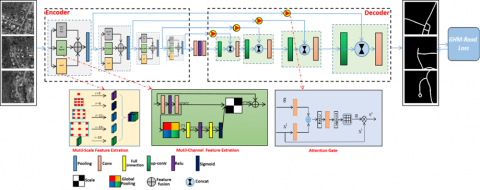
This paper proposes a Multi-scale Residual Attention U-Net for Road Detection (MRAU) network structure (Figure 6).
Figure 6. MRAU architecture frame
The MRAU structure mainly includes (a) a U-net-based encoder decoder and a skip connection structure as the backbone of the network structure to achieve end-to-end automatic segmentation and extract high-resolution remote sensing road images. (b) In the encoder part, on the basis of the standard 3*3 convolution structure of the U-net network, each layer proposes a new structure-fusion feature extraction module, including a spatial multi-scale feature extraction sub-module, a multi-channel feature extraction sub-module, and a deep learning feature extraction sub-module. The three modules perform feature learning on the input image in parallel and then perform feature fusion. (c) In the decoder part, the output of the symmetry layer in the process of feature extraction is applied and the feature is restored through the improved attention skip connection. (d) Loss function based on the gradient density coordination mechanism.
The MRAU network proposed in this paper is a novel end-to-end network for the tasks of automatic road detection from high-resolution remote sensing images. The architecture frame is shown in Figure 6. The backbone network of the MRAU network is similar to that of the U-net network. The original image undergoes two main processing stages: encoder and decoder. The roads in the high-resolution remote sensing images are identified and output. The encoding process of the MRAU network proposed in this paper is similar to the contracting path of the standard U-net network, consisting of four fusion feature extraction blocks. The decoding process is similar to the expanding path of the U-net network, which is also composed of four modules to achieve up sampling and feature enhancement based on the attention mechanism. To effectively overcome the large imbalance between the pixel numbers of road and non-road features in high-resolution remote sensing images, the loss function of the gradient coordination mechanism GHM-C is adopted.
2.2.2 Fusion feature extraction
One of the main innovations of the MRAU network is the fusion feature extraction ability, which consists of four fusion feature extraction blocks in the decoding/down sampling processing stage (as shown in Figure 6). The fusion features here refer mainly to the fusion of spatial multi-scale features, spectral multi-channel features, and deep learning feature sub-modules.
Spatial multi-scale features are extracted using the atrous spatial pyramid pooling method. Before importing to the MRAU network, the original input images are pre-processed and resized to 256*256 pixels. The input images go through four fusion feature extraction modules in turn, and the image sizes of the modules are 256*256, 128*128, 64*64, and 32*32, respectively. The atrous space pyramid used in this paper adopts a four-level structure, and the atrous convolution kernels with magnification ratios of 1, 6, 12, and 18 are convolved with the input image, respectively, and then the convolution results of different sizes are fused and output.
Spectral multi-channel features are extracted using the squeeze-and-excitation network proposed by Hu et al. [24] in 2017 to build a spectral multi-channel feature extraction module. High-resolution remote sensing images usually have multiple different spectral channel data, such as three-channel (RGB) image data. The spectral multi-channel feature extraction module constructed in this paper first performs global pooling on each channel of the input image (3*256*256) to obtain the intermediate result (3*1*1). Each channel is squeezed using a fully connected layer with a squeeze coefficient of 16, yielding an intermediate result (3/16 *1*1). Then, the excitation operation is again used for each channel. Here, the excitation operation also uses a fully connected layer. The intermediate result is 3*1*1. Finally, the sigmoid activation function is used to obtain a normalized weight result between [0, 1] on each of the multiple channels and a scale operation is used to weight the normalized weight to the features of each channel. The above-mentioned squeeze-and-excitation network and the residual network are fused to extract multi-channel features of high-resolution remote sensing images.
The fusion feature extraction module in this paper includes a deep learning feature sub-module, which uses the fully convolutional neural network (FCN) structure of the U-net network proposed by Ronneberger et al. [22] and is specifically composed of two groups of 3*3 convolution + activation function (Figure 6).
2.2.3 Feature enhancement based on the attention mechanism
Another important innovation of the MRAU network is the improved skip connection between down sampling and up sampling in the U-net network. The skip connection structure enables U-net to fuse the feature maps of the corresponding position of the encoder on the channel during the up sampling process of each level. The advantage of this method is that more low-level information can be obtained during up-sampling and then the details in the original image can be recovered more perfectly and the segmentation accuracy can be improved. However, the disadvantage is redundant information. Compared with not using skip connection, the segmentation accuracy can be improved, but there is obviously room for improvement. Therefore, on the basis of skip connection, this paper draws on the attention gate method proposed by Ozan et al. [26] in 2018 and forms a feature enhancement and up sampling method based on the attention mechanism.
As shown in Figure 6, there are two inputs to the method in this paper, in which the output of the encoder corresponding layer is used as an input g through skip connection and the output of the previous layer of the decoder is used as another input, x1. First, g and x1 are, respectively, convolved at 1*1 and concatenate the output. Then, they perform Relu activation, 1*1 convolution, and Sigmoid activation on the concatenated output in turn. Finally, the size of the output is adjusted to be the same as the input of this layer through Resample, which is the attention parameter αi. The value of αi ranges from 0 to 1, and then αi is multiplied by the input of this layer (the corresponding elements are multiplied one by one) to obtain the feature output of this layer's attention enhancement.
In this paper, the up sampling (expanding path) consists of four layers and the feature enhancement output of each layer is as described above, corresponding to the down sampling (contracting path) process (Figure 6).
2.2.4 Loss function GHM-C Loss
The road image data in the high-resolution remote sensing image data account for a small proportion of the entire image data, which will cause an imbalance of positive and negative samples and difficult and easy samples used for training. Referring to the practice of Li et al. [27], and using the distribution relationship of difficult and easy samples, when the gradient is small, the number of samples is large, and when the gradient is moderate, the number of samples is relatively small. Samples with a small gradient can be multiplied by a suppression coefficient, and samples with a large gradient can be multiplied by an excitation coefficient, where the suppression coefficient and incentive coefficient are determined according to the gradient distribution of the samples. The loss function used in this paper is as follows:
$L_{G H M-C}=\sum_{i=1}^N \frac{L_{C E}\left(p_i, p_i^*\right)}{G D\left(g_i\right)}$ (7)
This paper is experimentally validated on two different datasets: the first dataset is the Massachusetts Roads Dataset [28] and the second is the Deep Globe [29] global satellite image road extraction competition dataset.
3.1 Massachusetts roads dataset
The Massachusetts Roads Dataset contains a total of 1171 remote sensing images with an image size of 1500*1500 pixels, each image covers an area of 2.25 square kilo-meters, and the entire Dataset covers about 340 square kilometers. This dataset was published in 2013 by the University of Toronto, Canada. The images were mainly obtained from the relevant areas of Massachusetts, USA, and the land features were mainly urban, suburban, and rural. In this paper, 351 images are selected from the Massachusetts Roads Dataset as the training set and 30 as test set. To speed up the training of the model and reduce the time spent in the training process, the data image is cropped to a size of 256*256 pixels in this experiment (as shown in Figure 7).
Figure 7. Images and road maps of the Massachusetts Roads Dataset
Figure 8. Images and road maps of the Deep Globe Dataset
3.2 Deep globe dataset
The Deep Globe Satellite Image Road Extraction Competition Dataset was provided by the American Digital GLobe Company in the global satellite image road ex-traction competition held in 2018. It was mainly obtained from Thailand, Indonesia, and India, covering a land area of 2220 square kilometers, containing a total of 8570 remote sensing images. To compare with the experiments on the Massachusetts Roads Dataset, in this paper, 312 images are selected from the dataset as the training set and 30 as the test set and the data image is cropped to 256*256 pixels (Figure 8).
4.1 Measurement approach
To quantitatively measure the performance of different road detection methods, this paper adopts three indicators: precision, recall, and F1. In the road recognition task, precision refers to the probability that the model will predict that all pixels belonging to the road are actually positive samples (that is, actually road pixels). The recall rate refers to the probability that the model will predict a positive sample in real road pixels (i.e., the prediction belongs to road pixels). The F1 value is a balance index obtained by using the harmonic mean combined with the recall rate and the precision rate, which is used to measure the performance of the classifier and classification algorithm.
A binary classification problem such as road detection has four situations in terms of the prediction results and actual results of the model, represented by TP, FP, TN, and FN.
TP: The model predicts road pixels as road pixels;
FP: The model predicts non-road pixels as road pixels;
TN: The model predicts non-road pixels as non-road pixels;
FN: The model predicts road pixels as non-road pixels.
Prices $=\frac{\mathrm{TP}}{\mathrm{TP}+\mathrm{FP}}$ (8)
Re call $=\frac{\mathrm{TP}}{\mathrm{TP}+\mathrm{FN}}$ (9)
$\mathrm{F}_1=\frac{2 * \text { Pr ecise } * \text { Recall }}{\text { Precise }+\text { Recall }}$ (10)
4.2 Experimental configurations
In this paper, the above two datasets are used for the training and validation of the experimental model and the Tensor flow 1.5 machine learning platform is used. The processor is Intel(R) Xeon(R) E7530, with the following parameters: 1.87 ghz, 64 GB memory, GPU 2 Tesla T4, 16 GB video memory, Centos7 operating system, Linux Version 3.10.0-1160.6.1.el7.x86_64.
For the Massachusetts and Deep Globe Datasets, the MRAU network is compared with fCN-8s [30], U-net [22], ResUNet [31], DenseUNet [32], ResUNet++ [33], Attention U-Net [26], and other methods. The training batch is set to 50, and the initial learning rate is set to 1*10-5.
4.3 Experimental results
4.3.1 Experiment 1
Experiment 1 is based on the Massachusetts Road Dataset, and the MRAU network is trained and compared with six network models, fCN-8s [30], U-net [22], ResUNet [31], DenseUNet [32], ResUNet++ [33], and Attention U-Net [26], on the same dataset. The visualization effect is shown in Figure 9, and the quantitative comparison is shown in Table 1.
Figure 9 is a visual comparison between the MRAU network and the six network models: fCN-8s [30], U-net [22], ResUNet [31], DenseUNet [32], ResUNet++ [33], and Attention U-Net [26]. The first column is the original image, the second column is the label, the third to eighth columns are the results of the six networks (fCN-8s, U-net, ResUNet, DenseUNet, ResUNet++, and Attention U-Net), and the ninth column dis-plays the results of the MRAU network in this paper. In Figure 9, the green-framed area is the area where the road is mistakenly identified as the background and the red-framed area is the area where the background is mistakenly recognized as the road.
Figure 9. The visual comparison of methods on the Massachusetts Road Dataset
Table 1. Quantitative comparison of methods on the Massachusetts Road Dataset
|
Method |
Image 1 |
Image 2 |
Image 3 |
Image 4 |
Average |
||||||||||
|
P |
R |
F1 |
P |
R |
F1 |
P |
R |
F1 |
P |
R |
F1 |
P |
R |
F1 |
|
|
U-net |
0.8645 |
0.9166 |
0.8898 |
0.9228 |
0.908 |
0.9153 |
0.9271 |
0.9102 |
0.9186 |
0.8972 |
0.9142 |
0.9056 |
0.9029 |
0.9123 |
0.9073 |
|
fCN-8s |
0.5912 |
0.6541 |
0.6211 |
0.5883 |
0.6222 |
0.6048 |
0.6012 |
0.6568 |
0.6278 |
0.6017 |
0.6681 |
0.6332 |
0.5956 |
0.6503 |
0.6217 |
|
ResUNet |
0.9023 |
0.8946 |
0.8984 |
0.8962 |
0.8744 |
0.8852 |
0.9079 |
0.9018 |
0.9048 |
0.8963 |
0.8712 |
0.8836 |
0.9005 |
0.8855 |
0.893 |
|
DenseUNet |
0.9422 |
0.9186 |
0.9303 |
0.9372 |
0.9116 |
0.9242 |
0.9412 |
0.9138 |
0.9273 |
0.9245 |
0.8985 |
0.9113 |
0.9363 |
0.9106 |
0.9233 |
|
ResUNet++ |
0.9443 |
0.9268 |
0.9355 |
0.9566 |
0.9435 |
0.95 |
0.9518 |
0.934 |
0.9428 |
0.9404 |
0.9205 |
0.9303 |
0.9483 |
0.9312 |
0.9396 |
|
Attention U-Net |
0.9509 |
0.9328 |
0.9418 |
0.9625 |
0.9487 |
0.9556 |
0.9573 |
0.9234 |
0.94 |
0.9601 |
0.9413 |
0.9506 |
0.9527 |
0.9365 |
0.9477 |
|
MRAU (ours) |
0.9487 |
0.9369 |
0.9428 |
0.9643 |
0.9525 |
0.9584 |
0.9574 |
0.9297 |
0.9433 |
0.9531 |
0.9493 |
0.9512 |
0.9559 |
0.9421 |
0.9489 |
Table 1 shows the quantitative comparison results between the network used in this paper and the six network models (fCN-8s, U-net, ResUNet, DenseUNet, ResUNet++, and Attention U-Net). The first to fourth columns displays the quantitative comparison results of four images, and the fifth column displays the comparison results of 30 test sets.
4.3.2 Experiment 2
Experiment 2 is based on the DeepGlobe Road Dataset. The MRAU network is trained and compared with six network models—fCN-8s [30], U-net [22], ResUNet [31], DenseUNet [32], ResUNet++ [33], and Attention U-Net [26] on the same dataset. The visualization effect is shown in Figure 10, and the quantitative comparison is shown in Table 2.
Figure 10 is a visual comparison between the MRAU network and the six network models of fCN-8s [30], U-net [22], ResUNet [31], DenseUNet [32], ResUNet++ [33], and Attention U-Net [26]. The first column is the original image, the second column is the label, the third to eighth columns display the results of the six networks (fCN-8s, U-net, ResUNet, DenseUNet, ResUNet++, and Attention U-Net), and the ninth column dis-plays the results of the MRAU network in this paper. In Figure 10, the green-framed area is the area where the road is mistakenly identified as the background and the red-framed area is the area where the background is mistakenly recognized as the road.
Table 2 shows a quantitative comparison between the network in this paper and six network models: fCN-8s, U-net, ResUNet, DenseUNet, ResUNet++, and Attention U-Net. The first to fourth columns display the quantitative comparison results of four images, and the fifth column displays the comparison results of 30 test sets.
Figure 10. The visual comparison of methods on the Deep Globe Road Dataset
Table 2. Quantitative comparison of methods on the Massachusetts Road Dataset
|
Method |
Image 1 |
Image 2 |
Image 3 |
Image 4 |
Average |
||||||||||||
|
P |
R |
F1 |
P |
R |
F1 |
P |
R |
F1 |
P |
R |
F1 |
P |
R |
F1 |
|||
|
U-net |
0.9057 |
0.802 |
0.8507 |
0.9126 |
0.8574 |
0.8841 |
0.9185 |
0.8663 |
0.8916 |
0.9083 |
0.8282 |
0.8664 |
0.9113 |
0.8385 |
0.8734 |
||
|
fCN-8s |
0.6228 |
0.6847 |
0.6523 |
0.5871 |
0.625 |
0.6055 |
0.566 |
0.6128 |
0.5885 |
0.6042 |
0.6774 |
0.6387 |
0.595 |
0.65 |
0.6213 |
||
|
ResUNet |
0.8412 |
0.8127 |
0.8267 |
0.8161 |
0.7854 |
0.8005 |
0.8562 |
0.8497 |
0.8529 |
0.8263 |
0.8147 |
0.8205 |
0.835 |
0.8156 |
0.8252 |
||
|
DenseUNet |
0.9056 |
0.8932 |
0.8994 |
0.9145 |
0.8854 |
0.8997 |
0.9087 |
0.8853 |
0.8968 |
0.9204 |
0.8314 |
0.8736 |
0.9123 |
0.8738 |
0.8926 |
||
|
ResUNet++ |
0.914 |
0.7107 |
0.7997 |
0.9289 |
0.8332 |
0.8785 |
0.9271 |
0.8141 |
0.8669 |
0.9271 |
0.8141 |
0.8669 |
0.9243 |
0.793 |
0.8536 |
||
|
Attention U-Net |
0.9506 |
0.7685 |
0.8499 |
0.9654 |
0.7926 |
0.8705 |
0.9541 |
0.7573 |
0.8444 |
0.9401 |
0.7627 |
0.8422 |
0.9526 |
0.7703 |
0.8518 |
||
|
MRAU (ours) |
0.9225 |
0.9454 |
0.9338 |
0.9488 |
0.9482 |
0.9485 |
0.9431 |
0.9457 |
0.9444 |
0.9202 |
0.9526 |
0.9361 |
0.9337 |
0.948 |
0.9408 |
||
Experiment 1 shows that the FPs and FNs by the FCN are the most serious and there are many misidentifications. Compared with the fCN-8s network, the simple U-net network displays an improvement in FNs but the FPs are still serious and there are still many misidentifications. Compared with the FCN, there is a relative improvement in the FPs and FNs in the experimental results of the ResUNet network, but compared with the simple U-net network, there is a certain deterioration, which can also be seen from the comparison of quantitative data. In ResUNet, a skip connection is added to the simple U-net network and CLAHE enhancement is added. Here, the CLAHE enhancement operation does not eliminate the noise interference inside the ROI, which brings noise interference to the road recognition task and increases the FNs and FPs. In DenseUNet, the output of a certain layer is used as part of the input of several subsequent layers and the input of a certain layer results from the combination of the outputs of the previous layers. Through such a cross-layer output and input association structure, features extracted from different sizes are effectively used, which significantly improves FPs and FNs. The ResUNet++ network uses the atrous space pyramid pooling module connection between the encoder and the decoder and also uses the attention mechanism in the decoder part. The Attention U-Net network uses the attention mechanism in the skip connection between the same layer of the encoder and the decoder so that the output of the encoder part is processed by the attention mechanism to guide the decoder restoration process more accurately. Compared with FNs and FPs of the DenseUNet network, the improvement of the two networks is obvious. Compared with the Attention U-Net, the MRAU network proposed in this paper has significant improvements in FNs and FPs (Figure 9).
Similar to the results of Experiment 1, the FPs and FNs by the FCN are the most serious and there are many misidentifications. There is some improvement in terms of FNs and FPs by the simple U-net network but the FPs are still serious. Compared with the FCN, FPs and FNs are improved significantly in the ResUNet network. However, the ResUNet network is similar to Experiment 1 in the DeepGlobe Dataset, which also presents noise interference and increased FNs and FPs. Compared with fCN-8s, simple U-net, and ResUNet, DenseUNet and ResUNet++ display obvious improvements in FPs and FNs but there are still obvious misidentifications. Attention U-Net improves significantly in terms of FPs but still displays obvious FNs. In the network in this paper (Figure 10), the FNs and FPs have been significantly suppressed and the misidentified areas are significantly improved compared with the above six networks.
As can be seen from Table 1, the MRAU network proposed in this paper performs the best overall. In terms of precision index, the performance of the network in this paper is basically similar to that of Attention U-Net, but the recall rate and the F1 value are significantly improved. From the specific validation data, the precision index is as follows: Compared with fCN-8s, U-net, ResUNet, DenseUNet, ResUNet++, and Attention U-Net, the network in this paper has been improved by 36.03%, 5.3%, 5.54%, 1.96%, 0.76%, and 0.32%, respectively. Recall rate index: Compared with fCN-8s, U-net, ResUNet, DenseUNet, ResUNet++, and Attention U-Net, the network in this paper has been improved by 29.18%, 2.98%, 5.56%, 3.15%, 1.09%, and 0.56%, respectively. F1 value index: Compared with fCN-8s, U-net, ResUNet, DenseUNet, ResUNet++, and Attention U-Net, the network in this paper has been improved by 32.73%, 4.16%, 5.59%, 2.56%, 0.93%, and 0.12%, respectively (as shown in Figure 11).
Table 2 shows the results of a quantitative comparison between the network in this paper and the six network models of fCN-8s, U-net, ResUNet, DenseUNet, ResUNet++, and Attention U-Net. The first to fourth columns display the quantitative comparison results of four images, and the fifth column displays the comparison results of 30 test sets. In terms of precision index, compared with fCN-8s, U-net, ResUNet, DenseUNet, ResUNet++, and Attention U-Net, the network in this paper has been improved by 33.86%, 2.24%, 9.87%, 2.14%, 0.96%, and -1.89%, respectively. Recall rate index: Compared with fCN-8s, U-net, ResUNet, DenseUNet, ResUNet++, and Attention U-Net, the network in this paper has been improved by 29.80%, 10.95%, 13.24%, 7.42%, 15.5%, and 17.77%, respectively. F1 value index: Compared with fCN-8s, U-net, ResUNet, Dens-eUNet, ResUNet++, and Attention U-Net, the network in this paper has been improved by 31.95%, 6.74%, 11.56%, 4.82%, 8.72%, and 8.90%, respectively (as shown in Figure 12).
Figure 11. The accuracy of the quantitative results corresponding to different models in Experiment 1
Figure 12. The accuracy of the quantitative results corresponding to different models in Experiment 2
The above experiments show that the MRAU network does not improve the precision index significantly. For example, in Experiment 1, the method in this paper is only 0.32% better than Attention U-Net and even decreases compared with Attention U-Net in Experiment 2. However, the effect of the recall rate indicator is obvious. In Experiment 2, the recall rate of the network in this paper is 15.7% higher than the average value of other networks. The recall rate indicator is 17.7% higher than that of the Attention U-Net network. The MRAU network adopts the loss function based on the gradient coordination mechanism, which effectively suppresses the sample imbalance and significantly improves the recall rate of the model. In Experiment 1, as shown in Table 3, the MRAU network takes 244 min when training batch (epoch) = 50 and Attention U-Net takes 242 min when training batch (epoch) = 50. The MRAU network significantly improves the recall rate and the F1 value, while the time consumption does not increase.
Table 3. Quantitative comparison of time consumption
|
Epoch |
Attention U-Net(min) |
MRAU(min) |
|
10 |
51 |
49 |
|
20 |
93 |
98 |
|
30 |
150 |
147 |
|
40 |
200 |
198 |
|
50 |
242 |
244 |
This paper proposes the MRAU network for accurate road recognition in high-resolution remote sensing images by fusing the multi-scale, multi-channel, and depth residual learning features of road objects. At the same time, the up sampling process based on the attention mechanism of the proposed method combines the attention gate module with a skip connection, which further enhances the robustness and accuracy. Use of the optimized loss function based on the gradient coordination mechanism suppresses the imbalance of road samples in high-resolution remote sensing images and improves the recall rate significantly. Through detailed experimental verification of Massachusetts Roads and Deep Globe Datasets, compared with other road extraction methods, the proposed method provides more subtle insight into the road and does not increase the calculation.
In this paper, we found that the performance of different datasets is still slightly different. The reason is that the transfer learning ability of the proposed method needs to be strengthened. In the future, we will focus on how to enhance the versatility of road extraction methods from high-resolution remote sensing images and continuously improve the network model. In addition, the imbalance problem of road samples in high-resolution remote sensing images is typical in object detection and needs more insightful study to solve and improve in subsequent network models.
This work was supported by the National Natural Science Foundation of China (Grant No.: 52162050).
[1] Herold, M., Gardner, M.E., Roberts, D.A. (2003). Spectral resolution requirements for mapping urban areas. IEEE Transactions on Geoscience and Remote Sensing, 41(9): 1907-1919. https://doi.org/10.1109/TGRS.2003.815238
[2] Zhang, J., Feng, M.Q., Wang, Y. (2020). Automatic segmentation of remote sensing images on water bodies based on image enhancement. Traitement du Signal, 37(6): 1037-1043. https://doi.org/10.18280/ts.370616
[3] Ammour, N., Alhichri, H., Bazi, Y., Benjdira, B., Alajlan, N., Zuair, M. (2017). Deep learning approach for car detection in UAV imagery. Remote Sensing, 9(4): 312. https://doi.org/10.3390/rs9040312
[4] Cheng, G., Han, J. (2016). A survey on object detection in optical remote sensing images. ISPRS Journal of Photogrammetry and Remote Sensing, 117: 11-28. https://doi.org/10.1016/j.isprsjprs.2016.03.014
[5] Mnih, V., Hinton, G.E. (2010). Learning to detect roads in high-resolution aerial images. In Proceedings of the European conference on computer vision, Heraklion, pp. 210-223.
[6] Cheng, G., Zhu, F., Xiang, S., Pan, C. (2016). Road centerline extraction via semisupervised segmentation and multidirection nonmaximum suppression. IEEE Geoscience and Remote Sensing Letters, 13(4): 545-549. https://doi.org/10.1109/LGRS.2016.2524025
[7] Wu, L., Hu, Y. (2010). A Survey of Automatic Road Extraction from Remote Sensing Images. Acta Automatica Sinica, 36(7): 912-922. https://doi.org/10.3724/SP.J.1004.2010.00912
[8] Feng P., Cao F. (2015). Method of road information extraction in high resolution remote sensing images. Modern Electronics Technique, 38(17): 53-57.
[9] Zhao, W., Li-Qun, L., Zhou, G., Jun, Y., Wei, J. (2015). Road extraction in remote sensing images based on spectral and edge analysis. Spectroscopy and Spectral Analysis, 35(10): 2814-2819.
[10] Shi, W., Miao, Z., Debayle, J. (2013). An integrated method for urban main-road centerline extraction from optical remotely sensed imagery. IEEE Transactions on Geoscience and Remote Sensing, 52(6): 3359-3372. https://doi.org/10.1109/TGRS.2013.2272593
[11] Miao, Z., Shi, W., Zhang, H. (2013). A road centerline extraction algorithm from high resolution satellite imagery. Journal of China University of Mining & Technology, 42(5): 887-892.
[12] Que, H., Huang, H., Xu, J. (2014). Road edge detection based on dual-threshold SSDA template matching. Remote Sensing for Land and Resources, 26(4): 29-33. https://doi.org/10.6046/gtzyyg.2014.04.05
[13] Shanmugam, L., Kaliaperumal, V. (2016). Junction-aware water flow approach for urban road network extraction. IET Image Processing, 10(3): 227-234. https://doi.org/10.1049/iet-ipr.2015.0263
[14] Mu, H., Zhang, Y., Li, H., Guo, Y., Zhuang, Y. Road extraction base on Zernike algorithm on SAR image. In Proceedings of the 2016 IEEE International Geoscience and Remote Sensing Symposium (IGARSS), 2016; pp. 1274-1277.
[15] Tan, H., Huang, H., Xu, J. (2016). Road edge detection from remote sensing image based on improved Sobel operator. Remote Sensing for Land and Resources, 28(3): 7-11. https://www.gtzyyg.com/EN/Y2016/V28/I3/7
[16] Zeng, F., Yang, B., Wu, D., et al. (2013). Extraction of roads in mining area based on Canny edge detection operator. Remote Sensing for Land and Resources, 25(4): 72-78. https://doi:10.6046/gtzyyg.2013.04.12
[17] Cai, H., Yao, G. (2013). Optimized method for road extraction from high resolution remote sensing image based on watershed algorithm. Remote Sensing for Land and Resources, 25(3): 25-29. https://doi:10.6046/gtzyyg.2013.03.05
[18] Jin, J., Dang, J., Wang, Y., Zhai, F. (2017). Research on object oriented algorithm for road extraction in high-resolution remote sensing image. Journal of Lanzhou Jiaotong University, 36(6): 57-61. https://doi:10.3969/j.issn.1001-4373.2017.01.011
[19] Cheng, G., Zhu, F., Xiang, S., Pan, C. (2016). Road centerline extraction via semisupervised segmentation and multidirection nonmaximum suppression. IEEE Geoscience and Remote Sensing Letters, 13(4): 545-549. https://doi.org/10.1109/LGRS.2016.2524025
[20] Lu, X., Zhong, Y., Zheng, Z., Liu, Y., Zhao, J., Ma, A., Yang, J. (2019). Multi-scale and multi-task deep learning framework for automatic road extraction. IEEE Transactions on Geoscience and Remote Sensing, 57(11): 9362-9377.https://doi.org/10.1109/TGRS.2019.2926397
[21] Lu, X., Zhong, Y., Zheng, Z., Zhao, J., Zhang, L. (2020). Edge-reinforced convolutional neural network for road detection in very-high-resolution remote sensing imagery. Photogrammetric Engineering & Remote Sensing, 86(3): 153-160. https://doi.org/10.14358/PERS.86.3.153
[22] Ronneberger, O., Fischer, P., Brox, T. (2015). U-net: Convolutional networks for biomedical image segmentation. In Proceedings of the International Conference on Medical Image Computing and Computer-Assisted Intervention, Munich, pp. 234-241.
[23] He, K., Zhang, X., Ren, S., Sun, J. (2016). Deep residual learning for image recognition. In Proceedings of the Proceedings of the IEEE Conference on Computer Vision and Pattern Recognition, Las Vegas, pp. 770-778.
[24] Hu, J.; Shen, L.; Sun, G. (2018). Squeeze-and-excitation networks. In Proceedings of the Proceedings of the IEEE Conference on Computer Vision and Pattern Recognition, Salt Lake City, pp. 7132-7141.
[25] Chen, L.-C., Papandreou, G., Kokkinos, I., Murphy, K., Yuille, A.L. (2017). Deeplab: Semantic image segmentation with deep convolutional nets, atrous convolution, and fully connected crfs. IEEE Transactions on Pattern Analysis and Machine Intelligence, 40(4): 834-848. https://doi.org/10.1109/TPAMI.2017.2699184
[26] Oktay, O., Schlemper, J., Folgoc, L.L., Lee, M., Heinrich, M., Misawa, K., et al. Attention u-net: Learning where to look for the pancreas. arXiv preprint arXiv:1804.03999 2018.
[27] Li, B., Liu, Y., Wang, X. (2019). Gradient harmonized single-stage detector. In Proceedings of the Proceedings of the AAAI Conference on Artificial Intelligence, Palo Alto, pp. 8577-8584.
[28] Mnih, V. Machine learning for aerial image labeling; University of Toronto (Canada): 2013.
[29] Demir, I., Koperski, K., Lindenbaum, D., Pang, G., Huang, J., Basu, S., et al. (2018). Deepglobe 2018: A challenge to parse the earth through satellite images. In Proceedings of the Proceedings of the IEEE Conference on Computer Vision and Pattern, Salt Lake City, pp. 172-17209.
[30] Shelhamer E., Long J., T. Darrell. (2017). Fully Convolutional Networks for Semantic Segmentation. In IEEE Transactions on Pattern Analysis and Machine Intelligence, 39(4): 640-651. https://doi.org/10.1109/TPAMI.2016.2572683
[31] Xiao, X., Lian, S., Luo, Z., Li, S. (2018). Weighted res-unet for high-quality retina vessel segmentation. In Proceedings of the 2018 9th International Conference on Information Technology in Medicine and Education (ITME), Hangzhou, pp. 327-331.
[32] Huang, G., Liu, Z., Van Der Maaten, L., Weinberger, K.Q. (2017). Densely connected convolutional networks. In Proceedings of the IEEE Conference on Computer Vision and Pattern Recognition, pp. 4700-4708.
[33] Virnodkar, S.S., Pachghare, V.K., Patil, V.C., Jha, S.K. (2021). DenseResUNet: An architecture to assess water-stressed sugarcane crops from Sentinel-2 satellite imagery. Traitement du Signal, 38(4): 1131-1139. https://doi.org/10.18280/ts.380424