Feroz Morab* | Rajeshwari Hegde | Veena N. Hegde
© 2022 IIETA. This article is published by IIETA and is licensed under the CC BY 4.0 license (http://creativecommons.org/licenses/by/4.0/).
OPEN ACCESS
Accommodating multiple users within the limited available bandwidth and providing the same Quality of Service (QoS) to all the users is a challenging task. Channel capacity can be increased by using the Spatial Division Multiple Access (SDMA) technique. Smart Antenna Systems are used to implement the SDMA technique in Real-Time and it also helps in finding the high-resolution Direction of Arrival (DoA) detection of the desired mobile users. In this paper novel Gaussian Triangular Factor (GTF) method is proposed for the detection of the desired mobile users from the 3-D spatial domain. This method is based on vector subspaces, which perform the triangular decomposition of the entire Eigenspace into the Lower Element Factor (LEF) and Upper Element Factor (UEF). These are then supplied for the computation of the power spectrum where peaks represent the detected locations of the desired mobile users in the 3-D spatial field. The proposed method was able to detect all the desired users, which were spaced nearer or far apart spatially, it provided high-quality detection regardless of the number of antenna elements used at the Base Station (BS). The GTF Method was able to detect all the desired users under the presence of heavy noise, fading, and interference. It was able to suppress the side lobes, back lobes, and grating lobes thus immensely improving the detection quality, detection range, system power consumption, detection efficiency, and effectiveness. The proposed GTF method was compared with several existing methods and it provided the best results for different performance parameters like Detection Error, Resolution, Time Complexity, and Disturbance Error.
smart antennas, DoA, beamforming, phased antenna array, 5G, adaptive array antennas, mmWaves, 6G, array signal processing
In upcoming 5G and 6G wireless communication entire coverage area is divided into small number of picocells and femtocells. At each cell, Base Station (BS) is placed which consists of massive Multiple Inputs Multiple Outputs (MIMO) adaptive phased array antennas. The biggest challenge in these upcoming systems is how to accommodate multiple users within the scarcely available bandwidth at service provider’s disposal, how to accommodate multiple users in the same time frame and provide same QoS to all the users.
Thus, to overcome these issues Spatial Division Multiple Access (SDMA) technique is used, which accommodates multiple users within the same time frame and provides same QoS to all the users by separating them in different angular orientation. SDMA technology is based on smart antenna system, which helps in finding the Direction of Arrival (DoA) of desired mobile users from the 3-D spatial field.
Figure 1 shows the setup of Base Station Infrastructure with smart antenna systems, where the antenna elements are arranged in a linear sequence which have equal distance of separation from each other. The infrastructure uses Digital Signal Processor (DSP) which scans and reads incoming electromagnetic waves as digital signals and then process them to identify the direction of desired mobile users. Many classical DoA methods and vector subspace DoA methods were designed in the past but they all miserably failed to detect the desired users when they are spaced very closely to each other and they did not provide any reliable detection when BS was operating with the less number of antenna elements.
Figure 1. Base station infrastructure
Thus there is a dire need to solve this problem. This paper tries to solve this biggest problem of DoA detection by designing the robust and accurate algorithm that detects the desired users when they are closely spaced or widely spaced in the 3-D spatial domain, and to make effective detection possible when using less number of antenna elements or more number of antenna elements at BS. The proposed Gaussian Triangular Factor (GTF) method provides the detection of users under heavy noise, fading and interference. It also suppresses the side lobes and grating lobes to increase the main lobe gain and directivity to achieve the enhanced detection under the presence of random noise and fading.
This paper is organized as following: systematic and rigorous literature review was conducted which became the background of this research work it is presented in the Section-II; Section-III shows the design and implementation of proposed GTF method; Section-IV demonstrates the existing DoA methods; Experimental simulation results are presented in the Section V; Finally, Section-VI concludes the paper.
This section shows the systematic and rigorous literature survey that was conducted, this was used as the background material which acted as the cornerstone for the proposed research work.
The amplitude of electromagnetic waves falling at the base station is taken as a column vector along with Hermitian transpose by computing the auto-correlation matrix. The usage of amplitude values to find the power spectrum improves the accuracy [1].
The underwater detection of sources are done by computing the covariance matrix, which contains both the signal information and ambient noise. Singular Value Decomposition (SVD) is performed to suppress the ambient noise and to generate the noise subspace matrix using the computed eigenvalues and eigenvectors. The noise subspace is filtered out and then given for the power spectrum to compute the sharp detection peaks to give the location of the desired user in the spatial domain [2].
Leaky-wave array antennas are used for indoor as well outdoor mobile based communication. These antenna arrays are fabricated using four port based Substrate Integrated Waveguide (SIW). Two slot arrays along with the computation of radiation beams are solely based on the z-shaped junction that is formed by them. The main beams are directed towards the desired users by amalgamating the dual broad beams. Beam directions are determined by computing the phase shifts and weight vectors, which are connected to each of the individual antenna array elements [3].
The detection of the mobile users is done by computing the Angle of Arrival (AoA) which makes use of autocorrelation matrix along with the eigenvalues and eigenvectors. The Noise Subspace is generated using the eigenvectors on which the Multiple Signal Classification (MUSIC) algorithm is based. The energy computation is done by using the beam-width along the range, the phase shifts are computed by making use of array output along with error signals in such a way that minimum error is obtained, these phase shifts are then applied to individual sensor elements to form the main beam towards the user. This results in obtaining optimal Signal-to-Noise Ratio (SNR) value [4].
Sample Matrix Inverse (SMI) along with Least Mean Square (LMS) algorithms are used for the computation of the phase shifts. These phase shifts are applied to the individual sensor elements to form the main beams towards the desired users. The amplitudes of incoming signals at the Base Station is stored in a column vector, Signal correlation matrix is generated by the multiplication of amplitude vector along with the Hermitian transpose. The first phase shift is computed using the inverse of the resultant matrix, the error signals are computed using array output along with original signal [5].
For the communication link multiple sensors are used in both reception phase and transmission phase. During the reception phase, the detection of mobile users happens by using signal correlation matrix along with eigenvalues which are computed to measure and generate the subspaces, which are used to compute the power spectrum. The peaks of the power spectrum represent the user location in the spatial field. During the transmission phase, the computation of phase shifts, total received signal matrix and autocorrelation matrix is done which will be used to compute the step size. The new phase shifts are obtained by using phase shifts from previous iterations along with the step size, original signal and error signal; which is then applied to individual sensors to form the radiation towards the mobile user. The Constant Module (CM) along with Recursive Least Square (RLS) are used to form main beam [6].
Improved Variable-Step-Size LMS (I-VSSLMS) Algorithm enhances the DoA estimation capabilities. The (I-VSSLMS) algorithm beam-forming phase shifts are computed by making use of original signal, steering vector for specific direction, interference signals along with interference direction vectors and noise signal vector. The legacy power spectrum, makes use of auto correlation matrix to determine the power spectrum. Detection of the signals is performed by normalization of the phase shifts and computing inverse of the array pattern which leads to improved resolution of the legacy methods [7].
The Direction of Arrival (DoA) makes use of antenna arrays which are arranged in a nested form, the direction of mobile users is done by carrying out two different computations namely auto-correlation and cross-correlation. The polynomial is computed on the computed matrix to have the detection angles and then the resolution is used for the comparison of the different methods [8].
The demand for communication and value added services is increasing, thus to accommodate multiple users and to increase the capacity, SDMA Technique is used along with the multi antenna system which are configured as Uniform Circular Array (UCA) geometry. The MUSIC method will compute the auto correlation followed by the computation of the eigenvalues, for each eigenvalues the eigenvectors are computed. These eigenvalues are arranged in descending order and furthermore first (L-M) eigenvectors are combined together to form a low eigen subspace, where: (L) is the number of array elements, (M) is the number of desired vectors. This combination will result in the generation of the Noise subspaces, these noise subspaces are taken into consideration to compute the power spectrum, where the peaks represent the direction of the detected users [9].
Antenna array elements are arranged in a linear fashion with equal distance of separation between each element as , the individual antenna elements are either monopole or dipole antennas. The Capon Root-MUSIC algorithm computes the correlation matrix and the replicator matrix which is plugged in the power spectrum equation and then the transformation is done in order to detect the directions of sources [10, 11].
The reduction of noise values requires the execution of Taylor’s equation, which uses the offsets values to perform the Total Least Squares (TLS) computation. The system uses the nested antenna array to track the DoA which is based on offset compensation method. Along with these above specifications, the Discrete Fourier transform (DFT) is also used for the detection of desired sources [12].
Bayesian learning is applied for the linear array to compute the value of array manifold vector, likelihood functionality has the performance parameters such as size complexity and computational complexity which are used for detection of Angle of Arrival [13]. Antenna sensor array performs the signal processing at the Base Station to detect the direction of the incoming electromagnetic wave using Multiple Signal Classification (MUSIC) algorithm [14].
Steering vectors are computed using the Taylors method, weight vectors computations are based on the spatial computations using the grid model which utilize the IMUSIC method. Thus Bayesian inference is used to draw the inference about the detected direction of the desired user [15].
The smart antenna system produces the good estimation of directions if the compressed matrix along with the Sequential estimation method is applied to the Uniform Linear Array (ULA) which provides much better accuracy and thus improving the Root Means Square Error (RMSE) and resolution probability [16].
Mobile Source Detection (MSD) will find the location of the desired user and the location of the interference user. The computed data of MSD are used to generate beam shape patterns and these beam shapes are provided as input to the Method of Moments (MoM). The Signal-to-Interference and Noise Ratio (SINR) is improved by the combination of Mobile Source Detection (MSD) and Method of Moments (MoM) [17].
In the proposed method, the channel used by the mobile sources is based on the SDMA technique. In this technique, the capacity is improved by spatially sharing the channel with the multiple users. All the accommodated users operate at same frequency range within the same time frame but they are separated spatially which improves the capacity drastically because it has spatial dependency rather than frequency or time dependency. Among all the detection techniques, the subspace based technique is better as compared to the conventional technique because it allows to perform more complex signal processing techniques on the transmitting and receiving signals.
The proposed detection mechanism comprises of the following steps: (1) Computation of Total Correlation Matrix. (2) Computation of Eigenvalues. (3) Computation of Low Eigenspace. (4) Transformation of Gaussian Process and (5) Detection of Mobile Sources.
3.1 Computation of total correlation matrix
Consider the Uniform Linear Array (ULA) in which the elements are arranged in a sequence with equal distance between array elements.
Figure 2 shows the geometric layout of Uniform Linear Array, which has L number of individual antenna elements and each antenna element in an array is separated with a distance of $d=\lambda / 2$. This is the minimum separating distance required for proper detection and reducing the grating lobes.
The advantage of using multi-antenna array system at the Base Station over a single antenna system is that, it provides the improved SNR value by optimally combining all the signals and less signals are effected by the path loss and fading losses, thus the use of multi antenna array system improves the overall detection capabilities. When an electromagnetic wave hits the multi-antenna array system at the Base Station, it receives the original signal along with the several delayed copies of the same signal, even if few signals are corrupted the optimal combining of all the received signals will result in high SNR value.
Figure 2. Uniform linear array
The delay between the elements can be defined using the following equation:
$Dl{{t}_{i}}=\frac{i\,Dlv\,\sin {{\theta }_{s}}\,d}{TS(l)}$ (1)
where,
i=Positive number, Dlv=distance representation, $\theta_{s}$=direction of impinging Electromagnetic wave, d=distance between the antenna array elements.
The value of (i) will vary starting from 0 till the (Ne)th number of array elements.
The incoming electromagnetic waves contain original signal and multiple delayed copies of the same signal which are received at the different antenna elements at different time intervals from different directions. These values are stored as a column vector which has Ne number of rows as shown in Eq. (2).
$D_{v e m}(\theta)=\left[\begin{array}{c}1 \\ e^{-j \frac{2 \pi}{\lambda} d \sin (\theta)} \\ e^{-j(-2) \frac{2 \pi}{\lambda} d \sin (\theta)} \\ \vdots \\ e^{-j\left(N_{e}-1\right) \frac{2 \pi}{\lambda} d \sin (\theta)}\end{array}\right]$ (2)
where,
$\theta_{v}$=Signal Angle of Arrival, $\lambda$=Operating Wavelength, dis=Distance between Antenna elements.
In order to avoid the grating lobe, the distance between array elements should be multiple of half the operating wavelength $d=\lambda / 2$. By making use of half wavelength the disturbance can be avoided.
$D_{vem }(\theta)=\left[\begin{array}{c}1 \\ e^{-j \pi d \sin (\theta)} \\ e^{-j(-2) \pi d \sin (\theta)} \\ \vdots \\ e^{-j\left(N_{e}-1\right) \pi d \sin (\theta)}\end{array}\right]$ (3)
The base station processor needs to know the direction and the number of array elements in order to generate the delay vector representation.
If there are Nm number of mobile sources then the column vector of order (Nm x 1) is formed, which has Nm number of rows in it. Each row of this column vector represents the amplitude of electromagnetic wave hitting the individual antenna element at the Base Station.
$A_{v}=\left[\begin{array}{c}a m_{1} \\ a m_{2} \\ \vdots \\ a m_{N_{m}}\end{array}\right]$ (4)
where,
ami=The amplitude value for (i)th user.
The entire signal characteristics can be captured by forming the total Signal Correlation Matrix (SCM), which is generated by multiplying amplitude vector with its Hermitian transpose. The principle diagonal of SCM contains autocorrelation terms and off-diagonal contains cross-correlation terms.
$S C M=A_{v} * A_{v}^{H}$ (5)
By making use of Additive White Gaussian Noise (AWGN) the cross correlation terms between two different elements tend to zero.
$S C M=\left[\begin{array}{cccc}a m_{1} a m_{1}^{*} & 0 & \ldots & 0 \\ 0 & a m_{2} a m_{2}^{*} & \ldots & 0 \\ \vdots & \vdots & \ddots & \vdots \\ 0 & 0 & \ldots & a m_{N_{m}} a m_{N_{m}}^{*}\end{array}\right]$ (6)
The Noise Correlation Matrix (NCM) takes into consideration all the elements which are present at the Base Station. For the AWGN noise the total correlation noise matrix can be represented by using the following equation
$N C M=N_{v} * N_{v}^{H}$ (7)
The noise correlation matrix is generated by taking the noise vector and its Hermitian transpose, here each (nv) represents the noise contribution from each element with respect to the impinging electromagnetic waves.
$N C M=\left[\begin{array}{cccc}n v_{1} n v_{1}^{*} & 0 & \ldots & 0 \\ 0 & n v_{2} n v_{2}^{*} & \ldots & 0 \\ \vdots & \vdots & \ddots & \vdots \\ 0 & 0 & \ldots & n v_{N_{m}} n v_{N_{m}}^{*}\end{array}\right]$ (8)
For the random process which use the AWGN will have the same amplitude because the variance of the noise is almost equal as shown in the Eq. (9).
$n v_{1} n v_{1}^{*}=n v_{2} n v_{2}^{*}=\cdots=n v_{N_{m}} n v_{N_{m}}^{*}=\sigma^{2}$ (9)
By using the Eq. (9), the NCM can be represented as a product of identity matrix with variance of noise which is scalar value.
$N C M=\sigma^{2} I$ (10)
where,
$\sigma^{2}$=Variance of Noise, I=Identity Matrix.
If there are (Nm) number of mobile users then the array manifold vector is formed by combining the directional vectors from each of the direction and it is represented by using the following equation:
$A C M_{v}=\left\lceil A C M_{\theta_{1}} \quad A C M_{\theta_{2}} \quad \ldots \quad A C M_{\theta_{N_{m}}}\right\rceil$ (11)
The Total Correlation Matrix (TCM) captures the entire characteristics of the system, it is generated using the original signal, array manifold vector, signal correlation matrix and noise variance. The following equation shows the TCM:
$T C M=A C M_{v} * S C M * A C M_{v}^{H}+\sigma^{2} I$ (12)
where,
ACMv=Array Manifold Vector, ACMVH=Hermitian transpose of Array Manifold Vector, SCM=Signal Correlation Matrix, σ2=Noise Variance, I=Identity Matrix.
3.2 Computation of Eigenvalues
Eigenvalues are computed by solving the following equation.
$|T C M-\lambda I|=0$ (13)
where,
λ=Eigenvalue, ei=Eigenvector.
The solution to the Eq. (13) will provide the eigenvalues as $\left\{\lambda e_{1}, \lambda e_{2}, \ldots . ., \lambda e_{N_{e}}\right\}$ these eigenvalues should be sorted in ascending order of the magnitude values and then pick the first (Ne - Nm) terms.
3.3 Computation of Low Eigenspace
The Low Eigenspace will pick each of the eigenvalues and then compute the eigenvector for each eigenvalue as,
$TCM\,\,E{{V}_{n}}=\lambda {{e}_{i}}\,\,\,\,E{{V}_{n}}$ (14)
where,
TCM=Total Correlation Matrix, EVn=(Nex1) vector containing unknown values, λei=Eigenvalue.
$\left[ \begin{matrix} tr{{m}_{0,0}} & tr{{m}_{0,1}} & \ldots & tr{{m}_{0,Ne}} \\ tr{{m}_{1,0}} & tr{{m}_{1,1}} & \ldots & tr{{m}_{1,{{N}_{e}}}} \\ \vdots & \vdots & \vdots & \vdots \\ \,\,\,tr{{m}_{{{N}_{e}},0}} & tr{{m}_{{{N}_{e}},1}} & \ldots & \,\,\,\,\,\,tr{{m}_{{{N}_{e}},{{N}_{e}}}} \\\end{matrix} \right]\,\left[ \begin{matrix} E{{V}_{1}} \\ E{{V}_{2}} \\ \vdots \\ E{{V}_{{{N}_{e}}}} \\\end{matrix} \right]=\lambda e\left[ \begin{matrix} E{{V}_{1}} \\ E{{V}_{2}} \\ \vdots \\ E{{V}_{{{N}_{e}}}} \\\end{matrix} \right]\,$ (15)
Eigenvectors are obtained by solving the above Eq. (15) with a column vector of unknowns which has (Ne) number of rows.
$N S_{1}=\left[\begin{array}{c}e v_{11} \\ e v_{12} \\ \vdots \\ e v_{1 N_{e}}\end{array}\right]$ (16)
where,
ev1,j=The partial value element of eigenvector.
The (NS1) shows the generation of one such noise subspace, thus the entire Eigenspace is formed by combining the eigenvectors for all the (Ne) values.
$E V=\left[\begin{array}{cccc}e_{11} & e_{21} & \cdots & e_{N_{e} 1} \\ e_{12} & e_{22} & \cdots & e_{N_{e} 2} \\ \vdots & \vdots & \ddots & \vdots \\ e_{1 N_{e}} & e_{2 N_{e}} & \cdots & e_{N_{e} N_{m}}\end{array}\right]$ (17)
3.4 Transformation of Gaussian process
The transformation of Gaussian process is done by decomposing the entire Eigenspace into two different matrices such as Lower Elements Factor (LEF) and Upper Elements Factor (UEF). The Gaussian triangular factorization is computed using the following steps:
STEP 1: The formation of Lower Element Factor (LEF) matrix is done by making use of following
$L E F=\left[\begin{array}{cccc}1 & 0 & \ldots & 0 \\ L_{2} & 1 & \ldots & 0 \\ \vdots & \vdots & \ddots & \vdots \\ L_{N_{e} 1} & L_{N_{e} 2} & \ldots & 1\end{array}\right]$ (18)
STEP 2: The formation of Upper Element Factor (UEF) matrix is done by making use of following
$U E F=\left[\begin{array}{cccc}u_{e 11} & u_{e 12} & \ldots & u_{e 1 N_{e}} \\ 0 & u_{e 22} & \ldots & u_{e 12} \\ \vdots & \vdots & \ddots & \vdots \\ 0 & 0 & \ldots & u_{e N_{e} N_{e}}\end{array}\right]$ (19)
The combination of Lower Element Factor (LEF) and Upper Element Factor (UEF) is done in order to obtain the Gaussian Triangular Factor (GTF) method.
$G T F=L E F * U E F$ (20)
3.5 Detection of mobile locations
The detection of mobile user locations are done by combining both Lower Element Factor (LEF) and Upper Element Factor (UEF), these matrices are used in the computation of power spectrum where the peaks of power spectrum represent the locations of the desired users.
$P S_{G T F}=\frac{1}{D_{v}^{H}(\theta) * G T F G T F^{H} * D_{v}(\theta)}$ (21)
where,
Dv(θ)=Delay vector for direction θ, $D_{v}^{H}(\theta)=$Hermitian Transpose Delay vector for direction θ, GFT=Gaussian Triangular Factor, GTFH=Hermitian Transpose of Gaussian Triangular Factor.
In this section, the existing DoA methods are compared with the proposed scheme. The existing methods are bifurcated as Classical DoA Methods and Subspace DoA Method, the Classical DoA Method provides the detection based on simple signal processing techniques like Array Correlation Method (ACM), Maximum Magnitude Method (MMD) and Inverse Auto Correlation (IAC) Methods. The Subspace DoA Methods are implemented by generating the signal and noise subspaces, they allow the execution of complex signal processing techniques like Low Eigenvector Subspace (LEVS) method.
4.1 Array Correlation Method (ACM)
The array correlation is computed and then used directly for the detection. The spectrum is found for the range between -90° to + 90°, the peaks of the power spectrum show the detected directions of the mobile users.
$P S_{A C M}=\frac{D_{v}^{H}(\theta) * S C M * D_{v}(\theta)}{N_{E l e}^{2}}$ (22)
where,
Dv(θ)=Delay vector for direction θ, $D_{v}^{H}(\theta)=$Hermitian Transpose Delay vector for direction θ, SCM=Signal Correlation Matrix, NEle2=Number of Antenna Elements.
4.2 Maximum Magnitude Detection (MMD)
From all the columns of the correlation matrix, the column which has the highest magnitude is chosen as the column vector, this column vector is used in the detection of sources. The power spectrum is defined as the following.
$P S_{M M D}=\frac{1}{D_{v}^{H}(\theta) * M M M M^{H} * D_{v}(\theta)}$ (23)
where,
Dv(θ)=Delay vector for direction θ, $D_{v}^{H}(\theta)=$Hermitian Transpose Delay vector for direction θ, MM=Maximum Magnitude, MMH=Hermitian Transpose of Maximum Magnitude.
4.3 Inverse Auto Correlation Method (IAC)
The steering vector is computed for the desired directions and then combined with the array manifold vector, then the signal and noise correlation matrices are computed. The signal correlation matrix is obtained by combining the amplitude of electromagnetic waves along with its Hermitian transpose, the noise vector is computed by multiplying the noise vector along with its Hermitian transpose. Both the matrices are combined to form the total correlation matrix. The inverse of total correlation matrix is used in the power spectrum matrix and is defined as below.
$P S_{I A C}=\frac{1}{D_{v}^{H}(\theta) * T M C_{i n v} * D_{v}(\theta)}$ (24)
where,
Dv(θ)=Delay vector for direction θ, $D_{v}^{H}(\theta)=$Hermitian Transpose Delay vector for direction θ, TCMinv=Inverse of Total Correlation Matrix.
4.4 Low Eigenvector Subspace Method (LEVS)
The original signal along with delayed versions of the same signal are received at the Base Station, the auto correlation matrix is computed by taking the amplitudes of incoming electromagnetic waves. After that the noise correlation matrix along with array manifold vector is computed, these matrices are combined to form the total signal correlation matrix which is received at the Base Station. The eigenvalues are found for the total correlation matrix and then eigenvectors are found for each individual eigenvalue. Then the first (Na-Nm) eigenvectors are taken out and combined to form the noise subspace, this noise subspace is used in the computation of power spectrum and is provided by the following equation.
$P S_{L E V S}=\frac{1}{D_{v}^{H}(\theta) * N S N S^{H} * D_{v}(\theta)}$ (25)
where,
Dv(θ)=Delay vector for direction θ, $D_{v}^{H}(\theta)=$Hermitian Transpose Delay vector for direction θ, NS=Low Eigenvector Noise Subspace, NSH=Hermitian Transpose of Low Eigenvector Noise Subspace.
This section shows the experimental simulation results of the proposed method and along with that the comparisons with existing methods are done. The performance parameters that are used for the comparison between the algorithms are bias, resolution, time complexity, detection error and disturbance error. Bias gives the difference between what was estimated vs. what is actual detection direction, the resolution is the ability to detect the users which are closely spaced or spaced far apart.
To check the robustness and accuracy of each algorithm, they are tested for different cases such as:
Case1: Lesser Number of Antenna Elements and Widely Spaced Users Directions
Case2: Larger Number of Antenna Elements and Widely Spaced Users Directions
Case3: Lesser Number of Antenna Elements and Closely Spaced Users Directions
Case4: Larger Number of Antenna Elements and Closely Spaced Users Directions
5.1 Detection error
The detection error is the difference between the actual direction and the estimated direction.
$D E=\left|\theta_{Actual}-\theta_{Estimated} \quad \right|$ (26)
where,
θActual=Actual Direction, θEstimated=Estimated Direction.
5.2 Resolution
The resolution is the capability of the algorithm to detect and distinguish between two different users which are either closely spaced or spaced far apart in the 3-D spatial domain.
5.3 Case 1: Lesser number of antenna elements and widely spaced users directions
The Case-1 defines the condition when less number of antenna elements are used and the mobile users are spread-out in a wider directional space in the spatial field.
Table 1 shows the input configurations of the experimental setup, which uses less number of antenna elements i.e. 8 and the directions of the users are spaced wide apart in the 3-D spatial location of 10, 45 and 60 degrees.
Table 1. Detection experiment setup for case-1
|
Experimental Parameter |
Value |
|
Number of Array Elements |
8 |
|
Distance of Separation |
λ/2 |
|
Type |
Linear array |
|
Number of Sources |
3 |
|
Amplitude |
[1 2 3]v |
|
Actual Direction of Sources |
[10 45 60] degree |
Figure 3. AoA detection for case-1
Figure 3 shows the AoA detection for Case-1. The peaks in the power spectrum represents the detected direction of the desired users, the following methods such as MMD, LEVS, IAC and GTF were able to detect the directions of the users present at 10, 45 and 60 degrees, but the ACM method was unable to detect the directions of the mobile sources. The proposed GTF method provides the suppression of the side lobes, which improves the directivity of the main lobe and there will be lesser leakage of the energy via side lobes.
Table 2. Detection time for case-1
|
Algorithm |
Time Taken (ms) |
|
ACM |
0.7411 |
|
MMD |
0.7400 |
|
IAC |
0.7369 |
|
LEVS |
0.7386 |
|
GTF |
0.1619 |
Table 2 shows the Detection Time which represents the quickness of the algorithm in detecting the desired users from the spatial domain. The proposed GTF method has taken the lowest time to detect the sources then followed by the LEVS, IAC, MMD and ACM methods.
Table 3. Detection error for case-1
|
Algorithm |
Detection Error |
|
ACM |
0.7411 |
|
MMD |
0.7400 |
|
IAC |
0.7369 |
|
LEVS |
0.7386 |
|
GTF |
0.0193 |
Table 3 depicts the Detection Error which is the difference between what was actual direction to the detected direction form the algorithm, this error should be as low as possible. Here it can be clearly seen that the GTF method has very accurately estimated the locations of the desired users whereas existing DoA methods were unable to detect the users properly.
Table 4. Disturbance error for case-1
|
Algorithm |
Disturbance Error (w) |
|
ACM |
14000 |
|
MMD |
5010 |
|
IAC |
4345 |
|
LEVS |
3090 |
|
GTF |
1020 |
Table 4 represents the Disturbance Error, it shows how each algorithm is dealing with environmental and phenomenal disturbance such as thermal noise, system noise, AWGN, slow fading, fast fading, frequency selective fading, reflection and absorption effects. The proposed method delivered the lower disturbance error when compared to the existing DoA methods.
5.4 Case 2: Larger number of antenna elements and widely spaced users directions
The Case-2 shows the condition when larger number of antenna elements are used and the mobile sources are widely spaced in the spatial domain.
Table 5. Detection experiment setup for case-2
|
Experimental Parameter |
Value |
|
Number of Array Elements |
100 |
|
Distance of Separation |
λ/2 |
|
Type |
Linear array |
|
Number of Sources |
3 |
|
Amplitude |
[1 2 3]v |
|
Actual Direction of Sources |
[10 45 60] degree |
The input configuration for the experimental setup which uses larger number of antenna elements i.e. 100 are shown in Table 5, where users are located at 10, 45 and 60 degrees. The amplitude of incoming electromagnetic waves are [1 2 3]v.
Figure 4. AoA detection for case-2
Figure 4 shows the AoA Detection for Case-2. The proposed GTF method provides the exact detection of the location of the mobile sources which are widely spread-out in the free space at the following locations of 10, 45 and 60 degrees. The detection given by existing methods namely ACM, MMD, LEVS, IAC was not clean and some disturbance was present in there detection.
Table 6. Detection time for case-2
|
Algorithm |
Time Taken (ms) |
|
ACM |
0.8254 |
|
MMD |
0.8120 |
|
IAC |
0.9186 |
|
LEVS |
0.8058 |
|
GTF |
0.1621 |
Table 6 illustrates the time complexity of the different DoA algorithms for Case-2, by performing Gaussian triangular factorization on the entire Eigenspace the time required for detection of the mobile source is less for the proposed GTF method i.e. 0.1621 ms. The existing methods take more time to detect the source, the IAC algorithm has taken the highest time because computing the inverse operation is expensive.
Table 7. Detection error for case-2
|
Algorithm |
Detection Error |
|
ACM |
0.1156 |
|
MMD |
0.1149 |
|
IAC |
0.3539 |
|
LEVS |
0.3539 |
|
GTF |
0.0182 |
Table 7 shows the Detection Error, it represents how much error is present in algorithm's detection when compared to the actual direction of the user. The proposed GTF algorithm provides almost accurate detection of the users direction in the 3-D space when compared to the existing methods.
Table 8. Disturbance error for case-2
|
Algorithm |
Disturbance Error (w) |
|
ACM |
18742 |
|
MMD |
16000 |
|
IAC |
5000 |
|
LEVS |
3000 |
|
GTF |
1024 |
During the detection phase each algorithm experiences the disturbance which is a form of a random noise. For an effective and efficient detection to take place the disturbance error level should be low. Table 8 shows the disturbance error for detection of mobile sources by the various methods for Case-2, where proposed GTF method delivers the lowest value of the disturbance factor when compared with the existing DoA methods like LEVS, IAC, MMM and ACM, thus the ACM algorithm had the highest disturbance factor.
5.5 Case 3: Lesser number of antenna elements and closely spaced users directions
The Case-3 depicts the condition when lesser number of antenna elements are used and spacing between the mobile sources is narrow.
Table 9. Detection experiment setup for case-3
|
Experimental Parameter |
Value |
|
Number of Array Elements |
8 |
|
Distance of Separation |
λ/2 |
|
Type |
Linear array |
|
Number of Sources |
3 |
|
Amplitude |
[1 2 3]v |
|
Actual Direction of Sources |
[10 15 20] degree |
The parameters required for the experimental setup for Case-3 is as shown in Table 9, the system input configurations are as following: the spacing between the mobile sources is very narrow i.e. 10, 15 and 20 degrees, and lesser number of antenna elements are used.
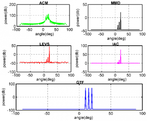
Figure 5. AoA detection for case-3
The majority of energy is leaked out via side lobes and grating lobes, for an efficient and effective detection these side lobes and grating lobes must be suppressed, the AoA detection for Case-3 is show in Figure 5. The proposed GTF method was able to detect all the mobile sources which are very closely spaced at 10, 15 and 20 degrees. The existing methods failed to detect these mobile sources which are so closely spaced.
Table 10. Detection time for case-3
|
Algorithm |
Time taken (ms) |
|
ACM |
0.7585 |
|
MMD |
0.7670 |
|
IAC |
0.7628 |
|
LEVS |
0.7672 |
|
GTF |
0.1658 |
Table 10 depicts the time complexity represents the amount of time taken by an algorithm to detect the mobile users in the free space, use of triangular factorization helps in reducing the timing complexity of the proposed GTF algorithm and MMD algorithm takes the highest time duration of 0.7670 ms.
Table 11. Detection error for case-3
|
Algorithm |
Detection Error |
|
ACM |
1.7110 |
|
MMD |
1.1380 |
|
IAC |
0.1328 |
|
LEVS |
0.0303 |
|
GTF |
0.0198 |
Table 11 shows the detection of estimated direction to the actual direction is given by the detection error, the lower detection error value provides the optimal and accurate detection rate for the algorithm. The least accurate detection was given by ACM algorithm and the proposed GTF method has provided more accurate and reliable detection thus it has the lowest detection error rate.
Table 12. Disturbance error for case-3
|
Algorithm |
Disturbance Error (w) |
|
ACM |
12944 |
|
MMD |
10161 |
|
IAC |
10153 |
|
LEVS |
8000 |
|
GTF |
1028 |
Similarly Table 12 represents the disturbance error factor of ACM algorithm is the highest and GTF has the lowest value of disturbance because it is least affected by it.
5.6 Case 4: Larger number of antenna elements and closely spaced users directions
The Case-4 defines the condition for larger number of antenna elements and the users are closely spaced in the spatial locations.
Table 13. Detection experiment setup for case-4
|
Experimental Parameter |
Value |
|
Number of Array Elements |
100 |
|
Distance of Separation |
λ/2 |
|
Type |
Linear array |
|
Number of Sources |
3 |
|
Amplitude |
[1 2 3]v |
|
Actual Direction of Sources |
[10 15 20] degree |
The experimental setup has the following input configurations such as the amplitude of incoming electromagnetic waves are [1 2 and 3]v and the mobile users are located very close to each other at 10, 15 and 20 degrees. Table 13 shows the entire setup of the system for Case-4.
Figure 6. AoA detection for case-4
Figure 6 shows AoA Detection, the proposed GTF algorithm was able to detect all the mobile sources in the spatial domain, but the existing algorithms namely ACM and MMD method were able to detect only one direction and missed the rest of the directions.
Table 14. Detection time for case-4
|
Algorithm |
Time Taken (ms) |
|
ACM |
0.8048 |
|
MMD |
0.8125 |
|
IAC |
0.9066 |
|
LEVS |
0.8105 |
|
GTF |
0.1687 |
From Table 14 it can be seen that the proposed GTF method takes the lowest time to detect the desired users in the 3-D spatial field, the IAC algorithm takes the most time to detect the mobile users, Table 14 shows the different detection time values for different algorithms.
Table 15. Detection error for case-4
|
Algorithm |
Detection Error |
|
ACM |
0.1157 |
|
MMD |
0.1149 |
|
IAC |
0.7425 |
|
LEVS |
0.1170 |
|
GTF |
0.0194 |
The detection error was computed for Case-4 using different DoA methods which is shown in Table 15, the GTF method provided very accurate detection of the desired users thus it has the lowest detection error rate when compared to all the other existing methods.
Table 16. Disturbance error for case-4
|
Algorithm |
Disturbance Error (w) |
|
ACM |
187420 |
|
MMD |
16000 |
|
IAC |
5000 |
|
LEVS |
3000 |
|
GTF |
1025 |
Disturbance error was computed for all the algorithms and the results are depicted in Table 16, the GTF method showed strong resilience against disturbance and it was least affected by it when compared to other existing methods. The ACM has the highest disturbance error followed by IAC, LEVS and MMD algorithms, thus proposed GTF algorithm outperforms all the other existing DoA algorithms.
5.7 Time complexity comparison
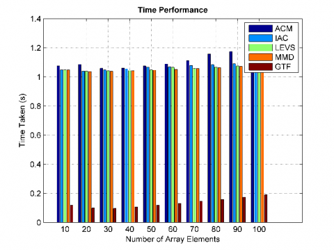
The time complexity comparison for all the algorithms were computed using different array count values ranging from 10 to 100 on x-axis and the time taken to detect is represented on the y-axis.
Figure 7 shows time complexity comparison for different algorithms, it represents the amount of time required by each algorithm to perform the detection of the desired mobile users from the 3-D free space. The proposed GTF method take the lowest time to perform the detection as compared to the LEVS, IAC, MMD and ACM methods.
5.8 Detection error comparison
Using different array count values ranging all the way from 10 elements to 100 elements the detection error for different algorithms were computed, where the array count values are represented on the x-axis and the amount of detection error values are shown on the y-axis.
Figure 7. Time complexity comparison
Figure 8. Detection error comparison
Figure 8 shows the different values of detection error for different algorithms, which are computed for varying array count values from 10 to 100. The ACM algorithm has highest detection error value because it was unable to estimate the user’s direction accurately and the proposed GTF method has shown the least value of the detection error because its estimation of desired users were accurate.
The SDMA technique was chosen to provide the communication access between the multiple Mobile Sources (MS) and Base Station (BS), because it provides the same frequency of operation to all the users in the same time frame but separating them spatially. Thus SDMA can accommodate multiple users with equal QoS therefore increasing the overall channel capacity and system performance. The proposed Gaussian Triangular Factor method was designed form the scratch and implemented. The GTF method was compared with existing DoA methods, experimental simulations were conducted under different environmental conditions and each of these algorithms were executed for different multiple cases to test their detection accuracy, robustness and time complexity.
To implement the smart antenna systems in real time, the proposed Gaussian Triangular Factor method plays a very vital role by providing high resolution DoA detection with less Bias and disturbance error. The GTF can detect the users which are spaced nearer or far apart and it can also provide excellent detection when using less number of antenna elements or more number of antenna elements at the BS. The Proposed GTF method successfully suppressed the side lobes and the grating lobes which caused the leakage of the energy and made the entire system less effective and less efficient. For each algorithm the power spectrum was computed and the peaks represented the location of the detected desired mobile users in the 3-D spatial field. Thus the proposed GTF method outperformed all the existing DoA methods and consistently delivered the best statistical results for different performance parameters such as Detection Error (0.019175), Detecting Resolution (very high), Time Complexity (0.164625 ms) and Disturbance Error factor (1024.25).
The work reported in this research paper is supported by the college through the Technical Education Quality Improvement Programme (TEQIP-III) of the MHRD, Government of India.
[1] Prince, T.J., Elmansouri, M.A., Filipovic, D.S. (2021). A framework for design of multibeam antenna systems used for amplitude-only direction finding based on correlation method. In 2021 IEEE-APS Topical Conference on Antennas and Propagation in Wireless Communications (APWC), pp. 109-109. https://doi.org/10.1109/APWC52648.2021.9539529
[2] Liu, A., Shi, S., Wang, X. (2021). Efficient DOA estimation method with ambient noise elimination for array of underwater acoustic vector sensors. In 2021 IEEE/CIC International Conference on Communications in China (ICCC Workshops), pp. 250-255. https://doi.org/10.1109/ICCCWorkshops52231.2021.9538869
[3] Li, X., Wang, J., Li, Z., Li, Y., Geng, Y., Chen, M., Zhang, Z. (2021). Leaky-wave antenna array with bilateral beamforming radiation pattern and capability of flexible beam switching. IEEE Transactions on Antennas and Propagation, 70(2): 1535-1540. https://doi.org/10.1109/TAP.2021.3111157
[4] Belay, H., Kornegay, K., Ceesay, E. (2021). Energy efficiency analysis of RLS-MUSIC based smart antenna system for 5G network. In 2021 55th Annual Conference on Information Sciences and Systems (CISS), pp. 1-5. https://doi.org/10.1109/CISS50987.2021.9400325
[5] Abualhayja'a, M., Hussein, M. (2021). Comparative study of adaptive beamforming algorithms for smart antenna applications. In 2020 International Conference on Communications, Signal Processing, and their Applications (ICCSPA), pp. 1-5. https://doi.org/10.1109/ICCSPA49915.2021.9385725
[6] Belay, H., Kornegay, K., Ceesay, E. (2021). Energy efficient smart antenna beamforming algorithms for next-generation networks. In 2021 IEEE 11th Annual Computing and Communication Workshop and Conference (CCWC), pp. 1106-1113. https://doi.org/10.1109/CCWC51732.2021.9376032.
[7] Qin, Y., Li, S., Tang, Z. (2021). DOA estimation method based on improved variable-step-size LMS algorithm. In 2021 International Symposium on Computer Technology and Information Science (ISCTIS), pp. 46-49. https://doi.org/10.1109/ISCTIS51085.2021.00018
[8] Sun, F., Lan, P. (2021). Efficient two-dimensional DOA estimation for coprime-displaced three parallel nested arrays. In 2021 6th International Conference on Communication, Image and Signal Processing (CCISP), pp. 393-397. https://doi.org/10.1109/CCISP52774.2021.9639271
[9] Alsalti, H.A., Abualnadi, D.I., Abdalazeez, M.K. (2021). Direction of arrival for uniform circular array using directional antenna elements. In 2021 IEEE Jordan International Joint Conference on Electrical Engineering and Information Technology (JEEIT), pp. 83-88. https://doi.org/10.1109/JEEIT53412.2021.9634136
[10] Tayem, N., Budimir, S., Veramareddy, V.R., Hussain, A.A. (2021). Capon root-MUSIC-like direction of arrival estimation based on real data. In 2021 IEEE 94th Vehicular Technology Conference (VTC2021-Fall), pp. 1-6. https://doi.org/10.1109/VTC2021-Fall52928.2021.9625275
[11] Yu, G.C. (2020). A computationally efficient estimation algorithm for direction of arrival in double parallel linear array. Traitement du Signal, 37(3): 443-449. https://doi.org/10.18280/ts.370311
[12] Zhang, Q., Li, J., Li, Y., Li, P. (2021). A DOA tracking method based on offset compensation using nested array. IEEE Transactions on Circuits and Systems II: Express Briefs, 69(3): 1917-1921. https://doi.org/10.1109/TCSII.2021.3114025
[13] Mao, Y., Guo, Q., Ding, J., Liu, F., Yu, Y. (2021). Marginal likelihood maximization based fast array manifold matrix learning for direction of arrival estimation. IEEE Transactions on Signal Processing, 69: 5512-5522. https://doi.org/10.1109/TSP.2021.3112922
[14] Sultan, K., Alharbey, R.A. (2019). ULA‐based near‐field source localisation in cognitive femtocell network: A comparative study of genetic algorithm hybridised with pattern search and swarm intelligence. IET Communications, 13(12): 1753-1761. https://doi.org/10.1049/iet-com.2018.5038
[15] Xu, X., Shen, M., Zhang, S., Wu, D., Zhu, D. (2021). Off-grid DOA estimation of coherent signals using weighted sparse Bayesian inference. In 2021 IEEE 16th Conference on Industrial Electronics and Applications (ICIEA), pp. 1147-1150. https://doi.org/10.1109/ICIEA51954.2021.9516237
[16] Bakhshi, G., Shahtalebi, K. (2017). Role of the NLMS algorithm in direction of arrival estimation for antenna arrays. IEEE Communications Letters, 22(4): 760-763. https://doi.org/10.1109/LCOMM.2017.2760253
[17] Chang, K.Y., Chen, K.T., Ma, W.H., Hwang, Y.T. (2019). An enhanced MUSIC DoA scanning scheme for array radar sensing in autonomous movers. In 2019 IEEE International Conference on Artificial Intelligence Circuits and Systems (AICAS), pp. 152-153. https://doi.org/10.1109/AICAS.2019.8771584