Zhenyu Wang | Mingshun Yang* | Leijie Ren | Jiali Han | Yirou Liu | Xingbai Zhao | Yangang Feng
© 2022 IIETA. This article is published by IIETA and is licensed under the CC BY 4.0 license (http://creativecommons.org/licenses/by/4.0/).
OPEN ACCESS
To detect the micro-size injection molded parts of electronic connectors, this paper establishes a complete size detection system based on machine vision, and measures the size through image acquisition and processing, according to the features of the injection molded parts. The proposed system is called the improved BM3D-Canny-Zernike algorithm. Specifically, the traditional block matching and three-dimensional filtering (BM3D) image denoising algorithm was improved to optimize the peak signal-to-noise ratio (PSNR) and reduce the mean squared error (MSE). Then, the Canny algorithm was improved for pixel-level edge detection, and the Zernike moment is improved for detecting edges on the subpixel-level more effectively and reducing the calculation amount. Finally, the least squares method was employed to fit the edge to be measured. The exact pixel length was obtained by solving the function of different edges, thereby realizing size measurement. Experimental results show that the mean error percentage of our algorithm was 8.73%, which meets the needs of industrial detection.
machine vision, size detection, image denoising, edge detection, block matching and three-dimensional filtering (BM3D)
Electronic connector, which connects the conductors in the circuit, is mainly produced through injection molding. The injection molded parts electronic connectors are easily affected by the mold, raw materials, and molding operation, and prone to suffer from depression, warpage deformation, and edge overflow. As a result, it is very difficult to directly measure the size of the electronic connector. Traditionally, the sample size is inspected manually with precision measurement tools. There are several disadvantages with the traditional approach, namely, difficulty in measurement, slow speed, low accuracy, and high missing rate. Thus, the traditional approach cannot meet the needs of automatic production. Introducing machine vision to geometric measurement can effectively avoid human errors, realize non-contact, precise, and efficient measurement, and automate the production and manufacturing process.
Researchers at home and abroad have extensively studied the online size measurement of parts, and made notable progress [1-4]. Different measurement protocols should be adopted depending on the type of parts, precision requirement, and processing condition. Injection molded parts are very small. Liu et al. [5] identified and measured particles as small as 1μm by scanning Raman microscopy. Gussen et al. [6] designed a multi-sensor measuring system for detecting plastic surfaces, and demonstrated that the system can measure the indicated properties of traditional materials and plastics. To calibrate cameras more effectively, Song et al. [7] relocated the subpixel edge of the feature points detected by the Canny operator, with the aid of Zernike. Zhang et al. [8] Combined ceramic slicing with deep learning to measure the thickness of fuel coating automatically and accurately. In general, pixel-level size detection is much more common than subpixel size detection. Focusing on subpixel size detection, Ren et al. [9] found that interpolation is susceptible to noise, and the smoothing effect of bilinear interpolation sacrifices the details and hinders high-precision detection.
During size measurement, two main problems may arise concerning the inspection of small-size parts. Firstly, the actual production environment is often unfavorable. The light, mechanical noise, and other factors may seriously affect the detection of part size. Secondly, it is difficult to extract subpixel edge features with sufficient accuracy. The existing studies on image denoising and edge detection mainly employ two kinds of methods: traditional methods [10-17], and deep learning-based methods [18-25]. With a fixed threshold, the traditional methods cannot adapt to the image scene with flexible noise and edge changes. Deep learning-based methods can solve the problem, but requires high-quality hardware, incurs heavy computation, and faces deployment difficulties [26].
To realize real-time precise detection of the size of injection molded parts of electronic connectors, this paper firstly improves the traditional block matching and three-dimensional filtering (BM3D) algorithm by introducing the flexible threshold of deep learning. Next, the Canny algorithm was improved to overcome the difficulty and high time cost of locating the edge center pixel, facilitating the pixel-level detection of edges. After that, ideal step model of Zernike moment was improved to detect subpixel edges more accurately, reflecting the smooth change of edge pixels in the actual image.
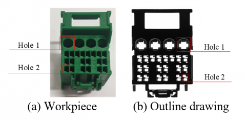
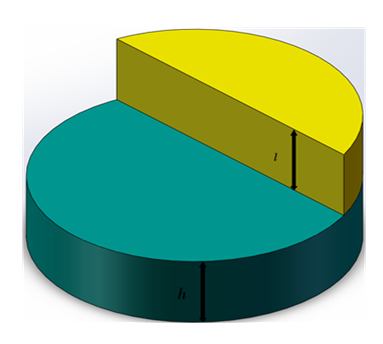
Figure 1 shows the shell of electronic connectors. The hole to be measured is a through hole. Back panel light was taken as the light source, and object telecentric lens were employed to acquire high-quality images.
Figure 1. Electronic connector
Image acquisition is often affected by noise, which hinders the extraction of the edge information from the small features of electronic connectors. Therefore, the first step of image preprocessing is denoising. This paper firstly denoises the original image by the BM3D algorithm, and then calls the Canny algorithm to extract the edge of the denoised image. Finally, Zernike moment was used to detect the subpixel positions of each edge of the image, laying the basis for subsequent size measurement.
2.1 Image denoising
The noise level of the original image directly affects the accuracy of edge extraction. Each common denoising algorithm has its unique features. Specifically, the mean filter and Gaussian filter blur the edge of the image, and are thus disqualified for size measurement. Despite its good boundary value, the median filter cannot effectively suppress the Gaussian noise. BM3D algorithm [27] can remove noise effectively without distorting image edges. That is why BM3D algorithm is selected for image denoising in this research.
2.1.1 BM3D
(1) Overview
The original BM3D algorithm converts every pixel of image from the spatial domain to frequency domain, before identifying and removing noise. Unlike ordinary spatial domain filters, BM3D can pinpoint and eliminate noises that cannot be detected in the spatial domain, but in the transformation domain of the basic estimate. The algorithm relies on a hard threshold to filter the noise pixels. In the actual detection environment of the electronic connector, each image has a unique gray value distribution, according to the analysis of noise sources. The noise in the image mainly comes from the high-frequency region, and approximates Gaussian noise. This calls for a method to remove high-frequency noise according to gray value distribution. To this end, we improved the BM3D algorithm.
(2) Improved BM3D Algorithm
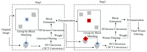
The BM3D algorithm has a much better noise reduction effect than spatial domain filters. But it might miss some image details of the Gaussian noises. To solve the problem, adaptive denoising was improved to enhance the removal of the high-frequency noise generated by the small feature size detection system of electronic connectors. The improved BM3D algorithm contains two steps, namely, basic estimation and final estimation. Each step involves three modules: similar block grouping, collaborative filtering, and aggregation. The overall flow chart of the algorithm is shown in Figure 2.
The improved BM3D algorithm uses Gaussian function instead of hard threshold. Since BM3D converts the target block into a 3D matrix, the 3D Gaussian function is called:
$\lambda _{3D}^{func}\left( {{f}_{x}},{{f}_{y}},{{f}_{z}} \right)=\lambda _{3D}^{hard}{{e}^{-\frac{f_{x}^{2}+f_{y}^{2}+f_{z}^{2}}{2{{\sigma }^{2}}}}}$ (1)
where, $\lambda_{3 D}^{\text {hard }}$ the hard threshold in the basic estimate, which depends on $f_{x}^{2}+f_{y}^{2}+f_{z}^{2} ; f_{x}^{2}+f_{y}^{2}+f_{z}^{2}$ the 3D coordinates in the transformation domain; σ is the standard deviation of a function, whose value is adjustable but independent of the noise level. Since the Z-axis data are not sorted in the grouping of target blocks, it is necessary to determine whether the frequency in the Z-axis direction is meaningful. Therefore, the denoising ability of BM3D algorithm should be compared here between two-dimensional (2D) Gaussian function and 3D Gaussian function.
$\lambda _{3D}^{func}\left( {{f}_{x}},{{f}_{y}},{{f}_{z}} \right)=\lambda _{3D}^{hard}{{e}^{-\frac{f_{x}^{2}+f_{y}^{2}}{2{{\sigma }^{2}}}}}$ (2)
The comparison shows that the improved BM3D far outperforms the traditional algorithm on images with rich details. However, the σ-values under different Gaussian noises differ significantly, and cannot be described by definite functions. In this paper, the relationship between Gaussian noise level and σ is summarized through multiple experiments. For ease of calculation, the relationship in Table 1 is adopted.
Figure 2. Flow chart of improved BM3D algorithm
Table 1. Coefficients σ under different levels of Gaussian noise
|
Gaussian noise level |
<40 |
40-60 |
80 |
100 |
|
σ |
8 |
10 |
12 |
16 |
Experimental results show that our algorithm excels, when the level of Gaussian noise falls between 40 and 100. At this time, the noise level is medium, the details of the high-frequency region are not covered, and the noise reduction is very effective. It can also be found that, although the Z-axis direction components are not ordered regularly in the 3D block area, the details have components on that axis. This means the noise also has components on the Z-axis. Then, it is imperative to remove the noise components on that axis. Hence, this paper selects a Gaussian function model with Z-axis denoising effect for cooperative filtering, instead of hard thresholding.
2.1.2 Results
In the real work environment, the image quality is mainly affected by illumination, human factors, and Gaussian noise. Therefore, our experimental processing focuses on the images under these three conditions. The noisy image is shown in Figure 3.
Figure 3. Noisy image
(1) Denoising effect in dark environment
In the actual production environment of electronic connectors, uneven or insufficient illumination may occur due to the problems of the light source on the factory pipeline. This study simulates the actual production environment in lab, and compares the denoising effect of original and improved BM3D on the electronic connector in dark environment.
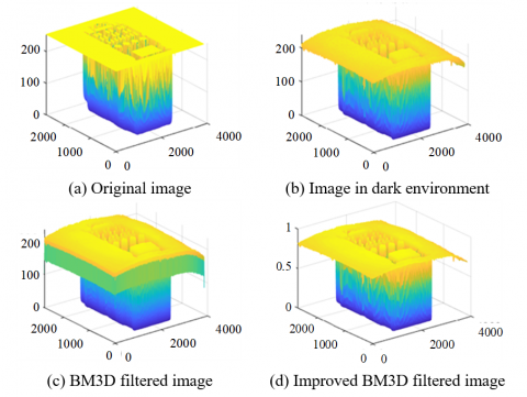
Figure 4. 3D histogram of denoising in dark environment
Figure 4 compares the 3D histogram effect of image denoising in dark environment. Comparing Figures 4(a) and 4(b), it is learned that the image data collected in dark environment are distorted by uneven and insufficient illumination. The size of smaller workpiece was affected more significantly. Comparing Figures 4(b) and 4(c), traditional BM3D greatly improved the quality of the image, but eliminated valuable information along with the noise, i.e., the noise removal is excessive. Comparing Figures 4(c) and 4(d), the improved BM3D effectively eliminated noise, while retaining the original information to the maximum extent. This is conductive to accurate edge detection.
(2) Denoising effect facing Gaussian noise
The contrast between samples from dark and light environments is not obvious enough. Therefore, we added Gaussian noise with a density of 0.3 to simulate the high-frequency noise generated by the electronic connector image acquisition system. Figure 5 presents the 3D histogram of denoising facing Gaussian noise. It can be seen that BM3D filtering generated a noise layer, while the improved BM3D approximated the histogram of the original image.
Figure 5. 3D histogram of denoising facing Gaussian noise
Figure 6. PSNR, MSE and SSIM values of different filters in dark environment
Figure 7. PSNR, MSE and SSIM values of different filters in manmade noise environment
(3) Evaluation of denoising quality
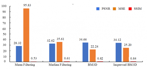
The 3D histogram can visualize the denoising effect of each algorithm. Here, the algorithm performance is evaluated objectively by noise reduction metrics, such as peak signal-to-noise ratio (PSNR), mean squared error (MSE) and structural similarity (SSIM) (Figures 6 and 7).
As shown in Figure 7, the improved BM3D increased PSNR, MSE and SSIM by 0.34%, 8.51%, and 2.8%, respectively, in the dark environment. When it comes to the manmade noise environment, the improved algorithm increased PSNR by 2.47%, reduced MSE by 29.36%, and increased SSIM by 3.58%. Obviously, the improved BM3D has a strong performance in noise removal.
2.2 Edge detection
Edge detection of objects is an important basis of size detection. Common edge detectors have various strengths and weaknesses. Sobel operator and Scharr operator are sufficient for common edge detection tasks. But they perform poorly in high-precision size measurement, where the detected edge is the aggregation of multiple pixels rather than a single pixel. Such an edge cannot be accepted as the calculation basis for size measurement algorithms on the pixel-level or even subpixel-level.
In feature extraction, the second-order Laplacian operator is more sensitive than the first-order Laplacian operator. The operator is also very sensitive to noise. However, the high sensitivity comes at the cost of a heavy computing load. In contrast, the Canny algorithm can locate edges accurately, pinpoint every pixel, and suppress the noise effectively. Nevertheless, this “ideal” edge detector has the following shortcomings: the image edges may be blurred by the Gaussian filter; the pixel gradient cannot be solved instantly by Gaussian function; the threshold selection lacks flexibility. Thus, the Canny algorithm is improved in the following subsection.
2.2.1 Improved Canny algorithm
Step 1. Denoise with improved BM3D.
Step 2. Extract image edge by Sobel operator.
Step 3. Carry out non-maximum suppression.
Step 4. Select the threshold by Otsu’s method [28], and connect the edge points through depth first search (DFS).
To sum up, the flow of the improved Canny algorithm is as follows: Firstly, the improved BM3D is used to filter the original image instead of Gaussian filter. Next, the Sobel operator is employed to calculate the gradient direction and gradient value. After that, non-maximum suppression is implemented based on computed gradient directions and gradient values. Then, the image is subject to thresholding, using the dual thresholds determined by Otsu’s method. After the processing based on the high and low thresholds, the edges are linked up through DFS.
2.2.2 Results
Illumination has a huge impact on image quality. Figure 8 compares the experimental results of Sobel operator, Canny algorithm, and improved Canny algorithm based on improved BM3D. It can be observed that the improved Canny algorithm achieved the best extraction effect on edge features, especially the small edge features. The extraction effect was much better than the original Canny algorithm.
2.2.3 Zernike moment operator
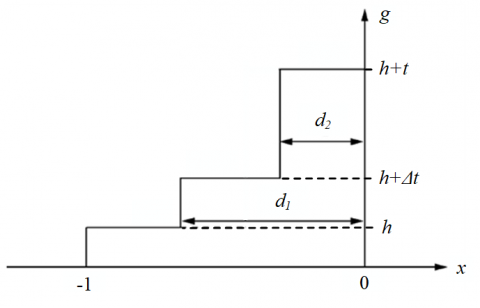
To detect subpixel edges, the traditional Zernike moment [29] assumes that the edge pixels of the original image have the same position information as those of the ideal step model. However, Figure 9 reveals that the pixels in the edge region of the ideal step model have abrupt gray values. By contrast, the edge region of the small features found in the actual image acquisition are not abrupt pixels, but gradually transit from the gray value of the background to the gray value of the edge region of the small features. There is a large difference in the moment between the actual edge region and the ideal step model. Thus, this paper improves the Zernike moment subpixel edge detection algorithm.
After analyzing the gray values of the pixels in the edge region of the actual image, a certain difference was noticed with the ideal step model: In the edge region of the tiny feature of the target electronic connector, the gray value is not an abrupt pixel, but gradually transits from the background gray value to the edge gray value. This paper adopts a three-gray interval model, which mimics the distribution of gray values in the edge region of the actual tiny features (Figure 10).
Figure 8. Results of different edge detectors in dark environment
Figure 9. Ideal edge step model
Figure 10. Three-gray interval model
Note: The solid line represents the three-gray interval model; the dotted line represents the ideal step model in the traditional Zernike moment method; h represents the gray value of the background; h + t represents the gray value of the edge region of the tiny feature; h +Δt represents the gray value change interval of the three-gray intervals; d1 represents the distance from the background to the edge pixels of the tiny feature; d2 represents the center distance between the three-gray intervals and the edge pixels of the tiny feature. Let a be the distance difference between d1 and d2. Then, d1 and d2 can be determined by edge features in the dark environment. Here, a 7×7 template is selected for a, i.e., a = 2/7.
The Zernike orthogonal moments can be calculated according to the three-gray interval model:
$\begin{align} & {{Z}_{00}}=\Delta t\left[ {{d}_{2}}\sqrt{1-d_{2}^{2}}+{{\sin }^{-1}}\left( {{d}_{2}} \right)-{{d}_{1}}\sqrt{1-d_{1}^{2}}- \right.\left. {{\sin }^{-1}}\left( {{d}_{1}} \right) \right] \\ & +t\left[ \frac{\pi }{2}-{{d}_{2}}\sqrt{1-d_{2}^{2}}-{{\sin }^{-1}}\left( {{d}_{2}} \right) \right]+h\pi \\\end{align}$ (3)
${{Z}_{11}}=\frac{2}{3}\Delta t\left[ {{\left( 1-d_{1}^{2} \right)}^{\frac{3}{2}}}-{{\left( 1-d_{2}^{2} \right)}^{\frac{3}{2}}} \right]+\frac{2}{3}t\left( 1-d_{2}^{2} \right)\frac{3}{2}$ (4)
${{Z}_{20}}=\frac{2}{3}\Delta t\left[ {{d}_{1}}{{\left( 1-d_{1}^{2} \right)}^{\frac{3}{2}}}-{{d}_{2}}{{\left( 1-d_{2}^{2} \right)}^{\frac{3}{2}}} \right]+\frac{2}{3}t{{d}_{2}}{{\left( 1-d_{2}^{2} \right)}^{\frac{3}{2}}}$ (5)
$\begin{align} & {{Z}_{31}}=\frac{2}{3}\Delta t\left[ {{\left( 1-d_{1}^{2} \right)}^{\frac{3}{2}}}-{{\left( 1-d_{2}^{2} \right)}^{\frac{3}{2}}} \right]+\frac{4}{5}\Delta t{{\left( 1-d_{2}^{2} \right)}^{\frac{5}{2}}} \\ & -\frac{4}{5}\Delta t{{\left( 1-d_{1}^{2} \right)}^{\frac{5}{2}}}+\frac{2}{15}t{{\left( 1-d_{2}^{2} \right)}^{\frac{3}{2}}}\left( 6d_{2}^{2}-1 \right) \\\end{align}$ (6)
Substituting the calculated values Z00, Z11, Z20, Z31 into the following Zernike moment template, a graph can be obtained for improved Zernike moment detection:
$\left[ \begin{array}{*{35}{l}} {{x}^{\prime }} \\ {{y}^{\prime }} \\\end{array} \right]=\left[ \begin{array}{*{35}{l}} x \\ y \\\end{array} \right]+\frac{N}{2}\cdot l\left[ \begin{array}{*{35}{l}} \cos (\phi ) \\ \sin (\phi ) \\\end{array} \right]$ (7)
where, (x’, y’) are the subpixel coordinates of the edge; (x, y) are the center of the unit circle; k, l and ϕ are parameters determined by Z11 and Z20.
The improved Zernike moment model optimizes the ideal step model of the traditional Zernike moment. The three-gray interval model was applied to the transition area of the edge region with a large background and tiny features, aiming to enhance the extraction ability of tiny feature edges and optimize the model. Unlike the traditional Zernike moment template, the improved Zernike moment template effectively speeds up subpixel detection, as it eliminates the need to compute Z40.
2.2.4 Comparative analysis on experimental results
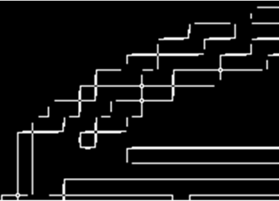
The holes to be inspected of the electronic connector is already shown in Figure 1. Figures 11 and 12 present the detection results of original and improved Zernike moment methods on holes 1 and 2, respectively.
(a) Detection results of Zernike moment method
(b) Detection results of improved Zernike moment method
Figure 11. Local contrast diagram for the two methods on hole 1
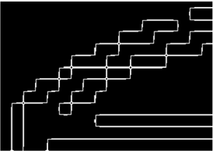
(a) Detection results of Zernike moment method
(b) Detection results of improved Zernike moment method
Figure 12. Local contrast diagram for the two methods on hole 2
The traditional Zernike moment method did not completely connect the edges, owing to the defect of the ideal step model. On the contrary, the results of the improved Zernike moment method contained no broken edges or discrete edge pixels, and featured completely connected edge regions. This is because the improved method connects the edge pixels smoothly according to the three-ray interval model. The improved Zernike moment method achieved the better recognition and positioning accuracy for different types of micro-feature edges of electronic connectors.
Figure 13. Flow of size detection system
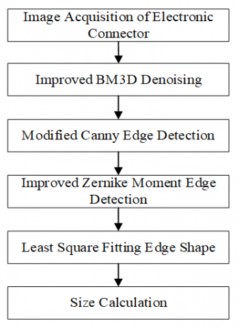
3.1 Size detection system
Figure 13 illustrates the process of size measurement. After acquiring the original image of the target workpiece, the image goes through preprocessing and edge extraction. Then, the key points are collected from the extracted data on the real edge. Afterwards, the polygonal edge function and circular function of the irregular workpiece are fitted by the least squared method, and the accurate pixel length is obtained by solving different functions. Finally, the error is analyzed in contrast to the actual measurements.
3.2 Edge fitting and size measurement
The points collected from the polygonal hole were fitted by the least squares method of the linear equation, while the tiny features of the target workpiece were piecewise fitted by the linear equation, in order to measure the edge length. In addition, the coordinates of the end points of each linear equation were obtained by connecting up the linear equations of all segments. In order to facilitate recording, the edge length is numbered as shown in Figure 14.
Based on the pixel size measured here, the mapping coefficient was solved and averaged at 65.5398. Then, the true size was obtained, and compared with the manually measured size of the workpiece, producing measurement error. In this paper, the measured pixel size is the mean of 50 groups of measured data. The experimental data are shown in Table 2.
Figure 14. Numbers of least squares fitting
Table 2. Experimental data on the size of target workpiece
|
Number |
Pixel size (pixel) |
Calculated size (mm) |
Measurement (mm) |
Measurement error (mm) |
Error percentage (%) |
|
C |
12 |
0.18 |
0.2 |
0.02 |
10.00 |
|
B |
25 |
0.38 |
0.5 |
-0.12 |
24.00 |
|
E |
54 |
0.83 |
1 |
-0.17 |
17.00 |
|
G |
60 |
0.92 |
1 |
-0.08 |
8.00 |
|
I |
63 |
0.96 |
1 |
-0.04 |
4.00 |
|
F |
87 |
1.33 |
1.5 |
-0.17 |
11.33 |
|
D |
96 |
1.46 |
1.5 |
-0.04 |
2.67 |
|
A |
119 |
1.82 |
1.8 |
0.02 |
1.11 |
|
H |
132 |
2.01 |
2 |
0.01 |
0.50 |
|
Mean |
72 |
1.10 |
1.17 |
-0.06 |
8.73 |
As shown in Table 2, when the measured size was below 0.9 mm, the relative error percentage was larger for relatively small edges C, B and E, peaking at 24.00%. With the increase of the measured size, the error percentage continued to decline. For the longest edge H, the error was only 0.50%. Referring to the size requirement of electronic connectors, the biggest error appeared at the edge lengths B and E, which does not significantly affect the functioning of the connector. Overall, the mean error percentage of size detection was 8.73%, which meets the requirements of industrial detection.
Focusing on the injection molded parts of electronic connectors, this paper specifically studies the detection of the tiny size of the holes. The acquired image was preprocessed before size measurement.
(1) In terms of image denoising, the traditional denoising algorithm may blur the image edge, which hinders edge extraction. This paper adopts the BM3D denoising algorithm to overcome the problem. But the hard threshold of the original BM3D cannot effectively eliminate the Gaussian noise in the high frequency region. Therefore, BM3D was improved for removing high-frequency noise. Using subjective and objective evaluation criteria, the images denoised by the original and improved BM3D were compared. The comparison shows the improved algorithm outperformed the original algorithm, and provides good quality denoised images for the subsequent edge detection process.
(2) In terms of pixel-level edge detection, the commonly used operators, e.g., Sobel operator, are discarded, due to its inaccurate localization of edge pixels, a fatal flaw for subpixel-level size measurement. The Canny algorithm can locate the edge pixel accurately, but falls short of the real-time requirement for industrial production lines. As a result, we improved the original Canny algorithm, and demonstrated through experiments that the improved algorithm can realize real-time detection of pixel-level edges.
(3) In terms of subpixel-level edge detection, this paper uses an optimization model, i.e., a three-gray interval model, instead of the ideal step model, and verifies that the improved Zernike moment method is more accurate for edge localization than the original method.
(4) The size of the target workpiece was measured in the following steps. Firstly, the linear and circular equations of the edges of tiny features were fitted by the least squares method. Then, the lengths of all sides of the polygon and the diameter of the circle were calculated. After that, the true physical sizes of the tiny features were computed by mapping the coefficients K. Finally, the measurement error was analyzed based on the measured results. The mean error percentage of experiments was merely 8.73%, which meets the industrial testing requirements.
(5) Our detection method has a high accuracy for the workpiece with relatively simple structure. However, the measurement accuracy of the parts with complex structure requires a comprehensive and systematic measurement of the parts. In future, the overall accuracy of a part will be considered, rather than measure the key sizes only.
This research is supported by National Natural Science Foundation of China (Grant No.: 52075437) and Natural Science Foundation of Shaanxi Province, China (Grant No.: 2021SF-422, 2021SF-421).
[1] Pai, W., Liang, J., Zhang, M.K., Tang, Z., Li, L. (2022). An advanced multi-camera system for automatic, high-precision and efficient tube profile measurement. Optics and Lasers in Engineering, 154: 106890. https://doi.org/10.1016/j.optlaseng.2021.106890
[2] Liu, Y., Mei, Y., Sun, C., et al. (2021). A novel cylindrical profile measurement model and errors separation method applied to stepped shafts precision model engineering. Measurement, 188: 110486. https://doi.org/10.1016/j.measurement.2021.110486
[3] Liu, W., Jia, Z., Wang, F., et al. (2012). An improved online dimensional measurement method of large hot cylindrical forging. Measurement, 45(8): 2041-2051. https://doi.org/10.1016/j.measurement.2012.05.004
[4] Li, X., Yang, Y., Ye, Y., Ma, S., Hu, T. (2021). An online visual measurement method for workpiece dimension based on deep learning. Measurement, 185: 110032. https://doi.org/10.1016/j.measurement.2021.110032
[5] Liu, D.T., Song, Y., Li, F.F., Chen, L.J. (2020). A detection method of small-sized microplastics based on micro-Raman mapping. Zhongguo Huanjing Kexue/China Environmental Science, 40(10): 4429-4438.
[6] Gussen, L.C., Ellerich, M., Schmitt, R.H. (2020). Equivalence analysis of plastic surface materials and comparable sustainable surfaces by a multisensory measurement system-sciencedirect. Procedia Manufacturing, 43: 627-634. https://doi.org/10.1016/j.promfg.2020.02.143
[7] Song, T., Tang, B., Zhao, M., Deng, L. (2014). An accurate 3-d fire location method based on sub-pixel edge detection and non-parametric stereo matching. Measurement, 50: 160-171. https://doi.org/10.1016/j.measurement.2013.12.022
[8] Zhang, H., Liu, J., Hu, Z., Chen, N., Yang, Z., Shen, J. (2022). Design of a deep learning visual system for the thickness measurement of each coating layer of TRISO-coated fuel particles. Measurement, 191(15): 110806. https://doi.org/10.1016/j.measurement.2022.110806
[9] Ren, Y.Q., Tu, D.J., Han, S. (2020). Dimension measurem-ent of diesel cylinder liner based on machine vision. Modular Ma-chine Tool & Automatic Manufacturing Tech-nique, 2020(9): 151-153. https://doi.org/10.13462/j.cnki.mmtamt.2020.09.034
[10] Thanh, D.N.H., Hien, N.N., Prasath, S. (2020). Adaptive total variation L1 regularization for salt and pepper image denoising. Optik, 208: 163677. https://doi.org/10.1016/j.ijleo.2019.163677
[11] Li, X., Meng, X., Xiong, B. (2022). A fractional variational image denoising model with two-component regularization terms. Applied Mathematics and Computation, 427: 127178. https://doi.org/10.1016/j.amc.2022.127178
[12] Routray, S., Malla, P.P., Sharma, S.K., Panda, S.K., Palai, G. (2020). A new image denoising framework using bilateral filtering based non-subsampled shearlet transform. Optik - International Journal for Light and Electron Optics, 216: 164903. https://doi.org/10.1016/j.ijleo.2020.164903
[13] Singh, H., Kommuri, S.V.R., Kumar, A., Bajaj, V. (2021). A new technique for guided filter based image denoising using modified cuckoo search optimization. Expert Systems with Applications, 176: 114884. https://doi.org/10.1016/j.eswa.2021.114884
[14] Hu, Q., Xu, X., Leng, D., Shu, L., Jiang, X., Virk, M., Yin, P. (2021). A method for measuring ice thickness of wind turbine blades based on edge detection. Cold Regions Science and Technology, 192: 103398. https://doi.org/10.1016/j.coldregions.2021.103398
[15] Ismael, A.A., Baykara, M. (2021). Digital image denoising techniques based on multi-resolution wavelet domain with spatial filters: A review. Traitement du Signal, 38(3): 639-651. https://doi.org/10.18280/ts.380311
[16] Bharodiya, A.K., Gonsai, A.M. (2019). An improved edge detection algorithm for x-ray images based on the statistical range. Heliyon, 5(10): e02743. https://doi.org/10.1016/j.heliyon.2019.e02743
[17] Li, N.N., Yue, S.Y., Jiang, B. (2020). Adaptive and feature-preserving bilateral filters for three-dimensional models. Traitement du Signal, 37(2): 157-168. https://doi.org/10.18280/ts.370202
[18] Xu, S., Zhang, J., Wang, J., Sun, K., Zhang, C., Liu, J., Hu, J. (2022). A model-driven network for guided image denoising. Information Fusion, 85: 60-71. https://doi.org/10.1016/j.inffus.2022.03.006
[19] Onishi, Y., Hashimoto, F., Ote, K., Ohba, H., Ota, R., Yoshikawa, E., Ouchi, Y. (2021). Anatomical-guided attention enhances unsupervised PET image denoising performance. Medical Image Analysis, 74: 102226. https://doi.org/10.1016/j.media.2021.102226
[20] Rajesh, C., Kumar, S. (2022). An evolutionary block based network for medical image denoising using differential evolution. Applied Soft Computing, 121: 108776. https://doi.org/10.1016/j.asoc.2022.108776
[21] Khowaja, S.A., Yahya, B.N., Lee, S.L. (2021). Cascaded and recursive convnets (crcnn): An effective and flexible approach for image denoising. Signal Processing Image Communication, 90: 116420. https://doi.org/10.1016/j.image.2021.116420
[22] Wang, L., Shen, Y., Liu, H., Guo, Z. (2019). An accurate and efficient multi-category edge detection method. Cognitive Systems Research, 58: 160-172. https://doi.org/10.1016/j.cogsys.2019.06.002
[23] Yan, J., Zhang, L., Luo, X., Peng, H., Wang, J. (2022). A novel edge detection method based on dynamic threshold neural P systems with orientation. Digital Signal Processing, 127: 103526. https://doi.org/10.1016/j.dsp.2022.103526
[24] Wang, B., Chen, L.L., Zhang, Z.Y. (2019). A novel method on the edge detection of infrared image. Optik, 180: 610-614. https://doi.org/10.1016/j.ijleo.2018.11.113
[25] Dong, B., Zhou, Y., Hu, C., Fu, K., Chen, G. (2021). Bcnet: bidirectional collaboration network for edge-guided salient object detection. Neurocomputing, 437(4): 58-71. https://doi.org/10.1016/j.neucom.2021.01.034
[26] Yang D.P., Peng B., Al-Huda Z., Malik A., Zhai D.H. (2022). An overview of edge and object contour detection. Neurocomputing, 488: 470-493. https://doi.org/10.1016/j.neucom.2022.02.079
[27] Dabov, K., Foi, A., Katkovnik, V., Egiazarian, K. (2007). Image denoising by sparse 3-d transform-domain collaborative filtering. IEEE Transactions on Image Processing, 16(8): 2080-2095. https://doi.org/10.1109/TIP.2007.901238
[28] Canny, J. (1986). A computational approach to edge detection. IEEE Transactions on Pattern Analysis and Machine Intelligence, PAMI-8(6): 679-698. https://doi.org/10.1109/TPAMI.1986.4767851
[29] Hwang, S.K., Kim, W.Y. (2006). A novel approach to the fast computation of Zernike moments. Pattern Recognition, 39(11): 2065-2076. https://doi.org/10.1016/j.patcog.2006.03.004