Hadj Abdelkader Benghenia* | Hadj Slimane Zine-Eddine | Andrade Alexandre
© 2022 IIETA. This article is published by IIETA and is licensed under the CC BY 4.0 license (http://creativecommons.org/licenses/by/4.0/).
OPEN ACCESS
A new method is proposed for recognition of the sleep apnea-hypopnea syndrome (SAHS) using electrocardiograms (ECG) signal in order to find an alternative with the same performance of polysomnography (PSG). Heart rate variability (HRV) signals generated from an ECG signal are used to examine a wide range of indices. A novel aspect of this work is the use of a method to decompose the HRV spectrum into total power spectrum (TP), high frequency (HF), low frequency (LF) and very low frequency (VLF) sub-band signals, and correlates their energy content with sympathetic and parasympathetic activity. The HRV signal was decomposed using the continuous wavelet transform (CWT) followed by the inverse continuous wavelet transform (ICWT), and sub-band signals were extracted from 5-minute episodes. In this regard, the suggested technique provides novel indices based on the mean of small (1 to 5), medium (6 to 10) and large (11 to 20) time scales of multiscal dispersion entropy (MDE) for each sub-band signals. In order to choose the best classifier, the indices of the MDE are submitted to a t-test technique and categorized using three classifiers: decision trees (DT), support vector machines (SVM-RBF) and K-nearest neighbor (KNN). The proposed method is evaluated using the combination of Physionet Apnea–ECG database and the University College Dublin Sleep Apnea Database. Using a 10-fold cross validation technique, the SVM-RBF classification approach achieves an average sensitivity, specificity, and accuracy of 93.91%, 96.92% and 93.94%, respectively. The results demonstrate that the approach presented is as precise as the best contemporary methods investigated using the same ECG datasets.
electrocardiogram (ECG), sleep apnea-hypopnea events (SAHE), continuous wavelet transform (CWT), multiscal dispersion entropy (MDE), classifiers
Sleep apnea–hypopnea syndrome (SAHS) is a respiratory disease that causes partial or total closure of the upper airways while sleeping [1, 2]. Obstructive sleep apnea is accompanied by a decrease in oxygen levels in the blood, with airway obstruction (partial or complete closure) lasting for at least 10 seconds and up to 3 minutes. Therefore, the body makes an important effort to breathe, but the air does not pass through it [3]. Hypopnea is a 50% reduction in respiratory flow for at least 10 seconds, accompanied by a minimum 3% reduction in oxygen saturation [4]. The Sleep apnea-hypopnea index measures the number and limitations of apnea per hour during sleep. The severity of sleep apnea can be assessed: normal (<5), mild (5-15), moderate (15-30) and severe (>30) [5]. Polysomnography (PSG) is the most complete and accurate medical examination designed to record the various stages of sleep by capturing the body's electrical rhythms [6]. The PSG typically includes electrocardiogram (ECG), electrocardiogram (EOG), electromyography (EMG), electroencephalography (EEG), oximeters, nasal airflow, oral airflow, tracheal and chest cavity sounds. However, it has some disadvantages, such as cost and patient discomfort [7]. As a result, devices and technologies that can somehow replace PSG are needed to detect SAHS. An electrocardiogram (ECG) is one of the primary signals used to screen for SAHS [8]. The effects of sleep apnea on the cardiovascular system have been observed indirectly. Therefore, it is possible to detect the consequences of obstructive sleep apnea in the cardiovascular system via the ECG signal. Changes caused by automatic and mechanical neurological factors in an electrocardiogram (ECG) could be a sign of recurrent apnea. In this case, there are periodic changes in the heart rate and the amplitude of the electrocardiogram or the morphology [9]. More specifically, studies have shown that HRV signal contains relevant information about OSA.
de Chazal et al. proposed an algorithm for automatic classification of periods of sleep apnea using ECG signals. The methodology of this study was based on the collection of 70 single-lead ECG results, half of which were used for training and the other half for test data. The 128 derived features based on estimates of the time and spectral domains of the HRV signal proved to be more insightful [10]. de Chazal et al. next used HRV and EDR signals to derive 88 simultaneous features in the time and spectral domains. The two classifiers used in this study are linear discrimination (LD) and quadratic discrimination (QD) [11]. Hossen et al. announced an automated method for detecting sleep apnea from HRV signals based on a sub-band decomposition soft decision algorithm [12]. Khandoker et al. extracted features from events of Hypopnea and wavelet based features and classified sleep apneas by using a two staged feed-forward neural network (NN) [13]. How OSA detects using empirical mode decomposition of ECG signal is by Mendez et al. proposed. In this study, minute apnea was classified using linear discrimination (LD) and quadratic discrimination (QD) as classifiers [14]. In another study proposed by a group of researchers, Bsoul et al. announce Apnea MedAssist, an app for real-time monitoring of apnea events that can detect obstructive sleep apnea. To train the SVM classifier, the time domain and frequency features are extracted from the RR intervals and the respiratory signals derived from the ECG [15]. Nguyen et al. use a nonlinear technique to analyze the HRV signal to detect OSA. Recurrence quantification analysis (RQA) is used to extract the hidden complexity present in the HRV signal [16]. Atri and Mohebbi demonstrated the effectiveness of combining linear and nonlinear methods in analyzing HR and EDR signals. They have developed an algorithm for OSA detection using new features based on bispectral analysis including spectra and HOS of HRV, EDR signals [17]. Janbakhshi and Shamsollahi proposed an approach to detect sleep apnea from features that rely on respiratory signals derived from an electrocardiogram (EDR) using various features in time and frequency domains and the ANN classifier [18]. The fluctuation properties of HRV were examined using fuzzy approximation entropy on 5-min HRV segments of OSA patients [19]. Feng et al. suggested unsupervised feature learning using an auto-encoder model. They employed the Hidden Markov Model (HMM) as a classifier and attained an accuracy of 85% [20].
Figure 1 depicts the general structure of the technique suggested in this research for screening OSA patients using HRV signal. In this work, twenty four new HRV signal indices are presented for SAHS recognition. These indices are calculated by taking the mean of the small (1 to 5), medium (6 to 10) and large (11 to 20) time scales of the MDE of sub-band signals described in this study. The suggested method begins by estimating the power spectrum of the HRV signal using the CWT methodology, from which the time-frequency spectrum picture is generated. Second, based on the physiological importance of HRV signal, the CWT image is split into several frequency bands, yielding many sub-scalograms. Third, the ICWT method is used to convert sub-scalograms into sub signals. Finally, twenty four unique indices are derived by examining the mean of the small, medium and large time scales of the MDE of various sub-band signals. In order to evaluate the performance of the proposed method for OSA screening, the decision tree (DT), support vector machine (SVM-RBF), and K-nearest neighbor (KNN) classifiers are applied to the twenty-four new indices.
Figure 1. Framework of the proposed method for sleep apnea-hypopnea events (SAHE) detection
2.1 The ECG data description
PysioNet is a physiological signal database that may be utilized in biomedical research. Both of the databases we utilized are accessible via the web site, allowing an easy examination and evaluation of our technique. The databases used in this research allow us to have more records in order to obtain different classes of SAHS [21].
2.1.1 The apnea-ECG database
This work uses the Apnea ECG database, which is available on the Physio website [8], to diagnose SAHS. The data consists of 70 recordings separated into a learning set (a01-a20, b01-b05, c01-c10) and a test set (x01-x35) with 35 records each. Each of these recordings is related to a single channel ECG signal (lead) with a sampling frequency of 100 Hz and a resolution of 16 bits, for a period of time (less than 7 h to approximately 10 h). Additionally, the ECG signals were collected based on the following factors: age, gender, weight, height, apnea index (AI), hypopnea index (HI), and apnea hypopnea index (AHI). They are classified into three groups based on the AHI value (a, b, c). When the AHI value is less than 5, it is classified as normal; when the value is greater than 10, it is classified as apnea; and when the value is less than 10, it is classified as boundary.
2.1.2 UCD database
The St. Vincent’s University Hospital/University College Dublin Sleep Apnea Database (UCD database) contains 25 complete overnight PSG records from people without heart disease or autonomic dysfunction and not taking any medication known to interfere with heart rate, each of which includes an ECG signal as well as other data. ECG signals are sampled at a rate of 125 Hz. Sleep technologists create annotations, which describe the onset and duration of all episodes of apnea and hypopnea. Two labeling standards are used to select the reference annotation on a one-minute basis. A similar method is used in the Apnea-ECG database. Each recording contains ECG signals that span 5.9 to 7.7 hours, as well as an annotation file that details the start time and length of each apnea or hypopnea event [22]. This database provides us with the options of normal and hypopnea groups.
2.2 Pre-processing
Accurate detection of the QRS complex is essential for producing optimal HRV signal from ECG recordings. The method we propose for the delineation of QRS complexes is based on a multi-resolution analysis by the wavelet transform. In wavelet applications, the mother wavelet chosen is extremely important. In reality, there is no well-defined criterion for selecting the mother wavelet, and this decision is highly dependent on the nature of the application and varies from one to the next. Several studies of wavelet analysis of the ECG signal have discovered that the 'Daubechies' wavelet family, specifically the wavelet 'db6,' is best suited for the treatment of the ECG signal since its form is comparable to the QRS complex [23].
As a result, the Daubechies mother wavelet ‘db6' will be used to breakdown the ECG signal throughout the remainder of this article. The level of decomposition chosen is also a factor to consider. In this algorithm, we have divided the ECG signal into nine levels [24]. This wise choice makes it possible to clearly distinguish the QRS complex, P waves, T waves and the baseline. The R peak detection is the most crucial stage in identifying the QRS complex since the accuracy of subsequent waves is dependent on this initial step. The db6 wavelet is used to produce nine levels of wavelet decomposition on the preprocessed ECG data. All information except D3 to D6 is preserved, while the rest are erased. The signal is therefore reconstructed from the details D3-D6, allowing the QRS complexes in the signal to be preserved while the other components at low and high frequencies are eliminated.
The Pan Tompkins method was used to identify the QRS complex from the previously filtered signal [25]. Once R peaks have been identified, HRV signal may be generated easily and precisely. The variation in successive RR intervals yields an HRV signal.
2.3 Feature description
2.3.1 Continuous wavelet transform (CWT)
The CWT is a robust time-frequency conversion method, which uses a set of wavelet functions to deal with simultaneous filtering and segmentation in the time-frequency domain. Unlike STFT, CWT is one of the most advanced methods for STFT, as it can provide by adjusting scale and translation parameters high time resolution and low frequency resolution in the high frequency, and high frequency resolution and low time resolution in the low frequencies [26]. The CWT can be computed from the following expression:
$\mathrm{X}_{\mathrm{CWT}}(\mathrm{u}, \mathrm{s})=\frac{1}{\sqrt{\mathrm{s}}} \int_{-\infty}^{\infty} \mathrm{x}(\mathrm{t}) \psi^{*}\left(\frac{\mathrm{t}-\mathrm{u}}{\mathrm{s}}\right) \mathrm{dt}$ (1)
where, s is a scale parameter, u is a translation parameter, and ψ*(t) is the mother wavelet. The scale can be converted to frequency by
$\mathrm{F}=\frac{\mathrm{F}_{\mathrm{c}} * \mathrm{f}_{\mathrm{s}}}{\mathrm{s}}$ (2)
where, Fc is the center frequency of the mother wavelet, fs is the sampling frequency of signal x(t) [27].
The synthesis of the complete or limited-range part of the signals is accomplished from the wavelet parameters by means of the inverse continuous wavelet transform (ICWT), defined as follows:
$x(t)=\frac{1}{C_{\psi}} \int_{-\infty}^{\infty} \int_{-\infty}^{\infty} X_{C W T}(u, s) \frac{1}{\sqrt{s}} \psi\left(\frac{t-u}{s}\right) d u \frac{d s}{s^{2}}$ (3)
where, Cψis the admissibility condition obtained when ψ(t) fulfills all the requirements to be considered a mother wavelet.
2.3.2 Multiscale dispersion entropy
Dispersion entropy (DisEn) is a time series irregularity measurement approach based on nonlinear dynamic analysis. DisEn has a better anti-noise capability than sample entropy since a slight change in amplitude does not modify the associated class label in DisEn.
The stages of DisEn may be stated as follows [28, 29] for a given univariate time series $X=\left\{x_{1}, x_{2}, \ldots, x_{N}\right\}$ with length N:
$y_{j}=\frac{1}{\sigma \sqrt{2 \pi}} \int_{-\infty}^{x_{j}} e^{\frac{-(t-\mu)^{2}}{2 \sigma^{2}}} d t$ (4)
where, $y i \in(0,1)$, and µ and σ represent the mean and standard deviation of time series X, respectively.
$\mathrm{z}_{\mathrm{j}}^{\mathrm{c}}=\mathrm{R}\left(\mathrm{c} \cdot y_{j}+0.5\right)$ (5)
where, $\mathrm{z}_{\mathrm{j}}^{\mathrm{c}}$ denotes the jth member of the classified time series, c means the number of classes, and R(·) represents the rounding function. Despite the fact that step (2) is linear, the entire mapping method is nonlinear due to the usage of NCDF in the first step.
Each time series $\mathrm{z}_{\mathrm{i}}^{\mathrm{m}, \mathrm{c}}$ can be mapped to a dispersion pattern $\pi_{v_{0} v_{1} \ldots v_{m-1}}$, where $\mathrm{z}_{\mathrm{j}}^{\mathrm{c}}=v_{0}, \mathrm{z}_{\mathrm{j}+\mathrm{d}}^{\mathrm{c}}=v_{1}, \ldots, \mathrm{z}_{\mathrm{j}+(\mathrm{m}-1) \mathrm{d}}^{\mathrm{c}}=v_{m-1}$. The number of possible dispersion patterns that can be assigned to each time series $\mathrm{z}_{\mathrm{i}}^{\mathrm{m}, \mathrm{c}}$ is equal to $c \mathrm{~m}$ as the signal has $m$ members, and each member can be one of the integers from 1 to $c$.
$p\left(\pi_{v_{0} v_{1} \ldots v_{m-1}}\right)=\frac{\#\left\{\begin{array}{c}\frac{i}{i} \leq N-(m-1) d, \mathrm{z}_{\mathrm{i}}^{\mathrm{m}, \mathrm{c}} \\ \text { has type } \pi_{v_{0} v_{1} \ldots v_{m-1}}\end{array}\right\}}{N-(m-1)}$ (6)
where, # means cardinality. In fact, $p\left(\pi_{v_{0} v_{1} \ldots v_{m-1}}\right)$ shows the number of dispersion patterns of $\pi_{v_{0}} v_{1} \ldots v_{m-1}$ that is assigned to $\mathrm{Z}_{\mathrm{i}}^{\mathrm{m}, \mathrm{c}}$, divided by the total number of embedded signals with embedding dimension m.
$\operatorname{DisEn}(\mathrm{X}, \mathrm{m}, \mathrm{c}, \mathrm{d})$
$=-\sum_{\pi=1}^{\mathrm{c}^{\mathrm{m}}} \mathrm{p}\left(\pi_{\mathrm{v}_{0} \mathrm{v}_{1} \ldots \mathrm{v}_{\mathrm{m}-1}}\right) \ln \left(\mathrm{p}\left(\pi_{\mathrm{v}_{0} \mathrm{v}_{1} \ldots \mathrm{v}_{\mathrm{m}-1}}\right)\right)$ (7)
It can be found from the algorithm of DisEn that when all distribution patterns $p\left(\pi_{v_{0} v_{1 \ldots} \ldots v_{m-1}}\right)$ have equal probabilities, DispEn acquires the largest entropy value $\ln \left(c^{m}\right)$, and a typical example is the Gaussian white noise.
In contrast, when the probability of the distribution pattern $p\left(\pi_{v_{0} v_{1 \ldots} \ldots v_{m-1}}\right)$ is unitary, i.e., only one value is not zero, DisEn obtains the smallest value, which indicates that the time series is completely predictable and a typical example is the periodic signal with low frequency.
According to DispEn, the MDE algorithm is as follows [29, 31]:
$\mathrm{y}_{\mathrm{j}}^{(\tau)}=\frac{1}{\tau} \sum_{\mathrm{a}=(\mathrm{j}-1) \tau+1}^{\mathrm{j} \tau} \omega_{\mathrm{a}}, 1 \leq \mathrm{j} \leq\lfloor\mathrm{L} / \tau\rfloor$ (8)
where, τ is called the scale factor and y(1) (i.e., $\tau=1$) is the original data. When $\tau>1$, the original data is divided into $\mathcal{T}$ coarse graining time series y(τ) with length ⌊N/τ ⌋ (where ⌊N/τ ⌋ represents the largest integral smaller than N/τ).
$\operatorname{MDE}(\mathrm{W}, \tau, \mathrm{m}, \mathrm{c}, \mathrm{d})=\operatorname{DE}\left(\mathrm{y}^{(\tau)}, \mathrm{m}, \mathrm{c}, \mathrm{d}\right)$
MDE analysis is the process of drawing DispEn over various time scales as a function of the scale factor. MDE corrects the flaws in DispEn, which only assesses time series irregularity on a single scale. The coarse graining-based multiscale method employed in MDE, on the other hand, is strongly reliant on the length of the time series, and the entropy fluctuation over many scales increases as the scale factor increases.
2.3.3 Sub-band signals extraction and nonlinear features
The CWT and ICWT methods were employed to extract the VLF, LF, HF, and TP sub-band-bands signal from the HRV signal. This approach is similar to separating the four bands of interest by using four independent band-pass filters with high cut-off frequencies, as demonstrated below [32]:
Nonlinear characteristics, such as multiscale dispersion entropy (MDE), are calculated from sub-band data. We computed the mean of the MDE values for each sub-band signal over three time scales: small (1 to 5), medium (6 to 10) and large (11 to 20).
2.4 Feature ranking
Feature rankings are used to select a subset of features. This reduces the complexity of the classifier without making a difference in performance. In our work, the feature raking method we have adopted is t-test. The student's t-test method is used to determine whether the mean of the two groups are different. The result of this test is the p-value of the calculated features of the two classes. The value of p is used to rank the features. Features with a low p-value are considered more discriminating [33]. Student's t-test raking was used to confirm differences between the normal and SAHS groups. At a p value of <0.01 the significance of the index was assumed. After ranking using the t-test technique, 24 characteristics for the identification of episodes of sleep apnea-hypopnea syndrome (SAHS) were retrieved from the Apnea-ECG and UCD databases.
2.5 Classification
2.5.1 Decision tree
The DT is a supervised classifier used to separate complex decision processes into simpler ones. This is a tree-like decision model built using the Input Training feature, in which each branch of the tree represents the result of the DT operation, the leaf nodes represent the class labels, and the attributes are specified by the internal nodes. The path from the root node of the tree to the leaf node depends on a set of rules for classification. Classifications rules help predict the class of unknown datasets [34].
2.5.2 k-nearest neighbor
The KNN classifier uses the relationship of the unknown sample to the nearest known sample to classify an unknown sample. Distance or similarity criteria are used to assess the proximity of the k-nearest sample [35]. Near samples are considered to be more effective than far-flung samples. Finally, the unknown sample is assumed to be a part of the same class as k-nearest neighbors.
2.5.3 Support vector machine
The SVM is one of the most widely used classifiers for constructing hyper-plane in feature space that divide training data into two categories [35]. If the data used is non-linearly separable, kernel functions can be used to map the original input data to a higher dimensional feature space and linearly separate the features. This study used least squares (LS-SVM) and radial basis functions (RBFs) to form decision boundary [36]. In this work, the highest classification accuracy was obtained considering the width σ of the RBF kernel function σ=3.1.
The HRV signals in the three classes: normal, OSA and hypopnea were examined using the recommended indices based on the CWT and MDE methods. To begin, all indices were evaluated the difference using the t-test. These 24 significant features were then assessed by three classifiers. These classifiers included the decision tree (DT), the support vector machine (SVM-RBF), and the K-nearest neighbor (KNN). To give more reliable and stable findings, the items were splited into testing and training sets using 10-fold cross validation, and the 10-fold cross-validation average was determined as the classification outcomes. In addition, three indices of precision (Acc), specificity (Spe) and sensitivity (Sen) were used to assess categorization outcomes, which are described as follows:
$\text { Accuracy }(\text { Acc })=\frac{\mathrm{TP}+\mathrm{TN}}{\mathrm{TP}+\mathrm{TN}+\mathrm{FP}+\mathrm{FN}}$
Specificity $( Spe )=\frac{\mathrm{TN}}{\mathrm{TN}+\mathrm{FP}}$
Sensitivity $(\mathrm{Sen})=\frac{\mathrm{TP}}{\mathrm{TP}+\mathrm{FN}}$
where, TN is the number of true negatives; TP is the number of true positives; FN is the number of false negatives; FP is the number of false positives.
In addition, 1000 minutes were chosen at random from each group for each experiment to increase the trustworthiness of the results (5430 minutes for OSA, 3000 minutes for respiratory impairment, and 9200 minutes for normal). In the last, the method was performed 100 times, and the average value of the results was the final result in the classification.
3.1 Results
The implementation of the proposed method was carried out in the MATLAB software. A total of 14630 episodes which includes normal and OSA, each episode of one minute duration is taken from 35 subjects of Apnea ECG database (20 subjects with recordings over 100 minutes of OSA, 5 subjects with recordings from 10 to 96 minutes of OSA and 10 subjects with less than 5 minutes of OSA), as for hypopnea episode, 3000 minutes were selected from UCD database. The noise for every minute of the ECG signal was deleted using a wavelet-based noise reduction technique. After noise reduction, QRS complex detection was performed using the Pan Tompkins algorithm. After detection of the QRS complex, HRV signal were obtained by calculating the time between two successive R peaks.
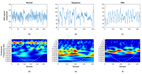
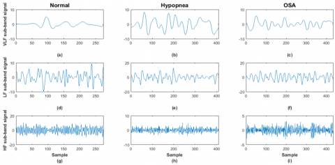
The TP, HF, LF and VLF sub-band signals were obtained by applying these three steps: first, converting the HRV signal into the time-frequency domain using a CWT technique as shown in Figure 2. Second, we have eliminated wave coefficients outside the VLF (0 to 0.04 Hz) or LF (0.04 to 0.15 Hz) or HF (0.15 to 0.4 Hz) or Total (0 to 0.4 Hz) bands by setting them to zero. Finally, the non-zero residual coefficients were converted to the time domain using ICWT technique to recover the spectral components. The HF, LF and VLF sub-band signals obtained by sequencing CWT and ICWT for a normal person and someone who suffers from OSA or hypopnea are shown in the Figure 3.
Using the proposed CWT followed by ICWT method with MDE analysis yielded a total of 24 indices. Eight indices are taken from mean of the small (1 to 5) time scales, and the rest are taken from the mean of the medium (6 to 10) and large (11 to 20) time scales. Table 1 shows the mean and standard deviation (SD) values for all groups. In addition, we calculated the p-value for both groups by using the t-test method.
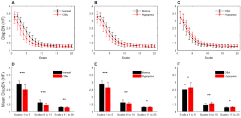
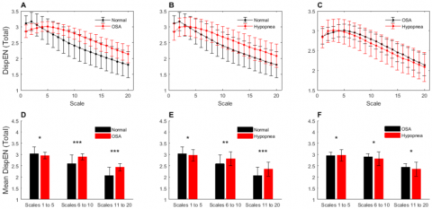
Figures 4-7 and Figure 8 represent the mean and standard deviation of the indices based on the method of calculating the MDE in the small (1 to 5), medium (6 to 10) and large (11 to 20) time scales of the sub-band signals. The 24 indices: DispEnVLF, DispEnLF, DispEnHF, DispEnTP, DispEnLF/HF, DispEnpVLF, DispEnpLF and DispEnpHF in the three time scales: small, medium and large were significantly different and varied as follows:
- Between normal and OSA episodes: 14 indices (p < 0.0001), 5 indices (p < 0.001) and 5 indices (p < 0.01).
- Between normal and hypopnea episodes: 6 indices (p<0.0001), 10 indices (p<0.001), and 8 indices (p<0.01).
- Between OSA and hypopnea episodes: 2 indices (p<0.0001), 6 indices (p<0.001), and 16 indices (p<0.01).
Figure 2. The five minute of HRV segment (up). 3D color power scalogram of HRV (down). The color represents the power scalogram. (a, d) Normal segment; (b, e) Hypopnea segment; (c, f) OSA segment
Figure 3. The VLF sub-band signal reconstructed by ICWT (left). LF sub-band signal reconstructed by ICWT (center). HF sub-band signal reconstructed by ICWT (right). (a, d and g) belongs to Normal episodes; (b, e and h) belongs to Hypopnea episodes; (c, f and i) belongs to OSA episodes
Table 1. Range distribution (mean ± standard deviation) of small, medium and large time scales of MDE features extracted from the TP, HF, LF and VLF sub-band signals using CWT followed by ICWT technique for normal, OSA and hypopnea episodes
|
Index |
Mean Scales |
Normal (Mean±SD) |
OSA (Mean±SD) |
Hypopnea (Mean±SD) |
p-value Normal–OSA |
p-value Normal-Hypopnea |
p-value OSA–Hypopnea |
|
DispEn_VLF |
Scales 1 to 5 |
2.9865 ± 0.1197 |
2.8563 ± 0.1827 |
2.8171 ± 0.1232 |
0*** |
0*** |
0* |
|
DispEn_LF |
2.9996 ± 0.1885 |
3.0955 ± 0.2464 |
3.0807 ± 0.1588 |
0* |
0* |
0.2050* |
|
|
DispEn_HF |
2.8755 ± 0.2198 |
2.4879 ± 0.3608 |
2.6272 ± 0.3297 |
0*** |
0*** |
0* |
|
|
DispEn_TP |
3.0280 ± 0.3043 |
2.9509 ± 0.1414 |
2.9634 ± 0.2592 |
0* |
0* |
0.3151* |
|
|
DispEn_LF/HF |
1.0464 ± 0.0721 |
1.2643 ± 0.1730 |
1.1906 ± 0.1602 |
0*** |
0*** |
0* |
|
|
DispEn_pVLF |
0.9985 ± 0.1321 |
0.9707 ± 0.0839 |
0.9603 ± 0.1192 |
0* |
0* |
0.1774* |
|
|
DispEn_pLF |
0.9984 ± 0.0952 |
1.0516 ± 0.0995 |
1.0495 ± 0.1282 |
0* |
0* |
0.8063* |
|
|
DispEn_pHF |
0.9553 ± 0.0745 |
0.8450 ± 0.1286 |
0.8928 ± 0.1344 |
0*** |
0** |
0* |
|
|
DispEn_VLF |
Scales 6 to 10 |
2.9685 ± 0.1243 |
3.0360 ± 0.1649 |
2.9777 ± 0.1305 |
0** |
0.1958* |
0** |
|
DispEn_LF |
1.9218 ± 0.2185 |
2.2381 ± 0.2492 |
2.1263 ± 0.2062 |
0*** |
0** |
0** |
|
|
DispEn_HF |
1.6115 ± 0.1852 |
1.4437 ± 0.1088 |
1.5277 ± 0.1072 |
0*** |
0** |
0** |
|
|
DispEn_TP |
2.5821 ± 0.4007 |
2.8954 ± 0.1401 |
2.8121 ± 0.3077 |
0*** |
0** |
0* |
|
|
DispEn_LF/HF |
1.1990 ± 0.1251 |
1.5547 ± 0.1747 |
1.3948 ± 0.1299 |
0*** |
0*** |
0*** |
|
|
DispEn_pVLF |
1.1859 ± 0.2500 |
1.0508 ± 0.0739 |
1.0761 ± 0.1674 |
0** |
0** |
0.4000* |
|
|
DispEn_pLF |
0.7594 ± 0.1260 |
0.7741 ± 0.0891 |
0.7682 ± 0.1369 |
0.1770* |
0.2603* |
0.4301* |
|
|
DispEn_pHF |
0.6372 ± 0.1054 |
0.4997 ± 0.0438 |
0.5516 ± 0.0869 |
0*** |
0*** |
0*** |
|
|
DispEn_VLF |
Scales 11 to 20 |
2.3984 ± 0.1990 |
2.6003 ± 0.1695 |
2.5259 ± 0.1415 |
0*** |
0** |
0** |
|
DispEn_LF |
1.3330 ± 0.0667 |
1.4093 ± 0.1024 |
1.3753 ± 0.1014 |
0** |
0* |
0* |
|
|
DispEn_HF |
1.3117 ± 0.0422 |
1.2860 ± 0.0382 |
1.3065 ± 0.0484 |
0** |
0.5170* |
0* |
|
|
DispEn_TP |
2.0588 ± 0.3697 |
2.4288 ± 0.1642 |
2.3457 ± 0.3148 |
0*** |
0*** |
0* |
|
|
DispEn_LF/HF |
1.0166 ± 0.0481 |
1.0959 ± 0.0736 |
1.0526 ± 0.0644 |
0*** |
0** |
0** |
|
|
DispEn_pVLF |
1.1975 ± 0.2120 |
1.0753 ± 0.1000 |
1.1030 ± 0.2105 |
0** |
0** |
0.1390* |
|
|
DispEn_pLF |
0.6703 ± 0.1346 |
0.5828 ± 0.0574 |
0.6014 ± 0.1254 |
0*** |
0** |
0.1900* |
|
|
DispEn_pHF |
0.6601 ± 0.1323 |
0.5320 ± 0.0416 |
0.5703 ± 0.1038 |
0*** |
0** |
0** |
|
|
*, ** and ***=p < 0.01, p < 0.001 and p < 0.0001, respectively |
|||||||
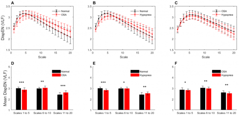
Figure 4. The computed multiscale dispersion entropy curves and Bar graphs for Normal & OSA (A and D), Normal & Hypopnea (B and E), and OSA & Hypopnea (C and F), which were obtained from the (VLF) signal
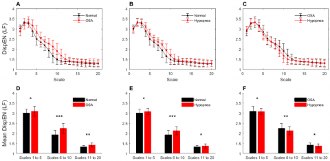
Figure 5. The computed multiscale dispersion entropy curves and Bar graphs for Normal & OSA (A and D), Normal & Hypopnea (B and E), and OSA & Hypopnea (C and F), which were obtained from the (LF) signal
Figure 6. The computed multiscale dispersion entropy curves and Bar graphs for Normal & OSA (A and D), Normal & Hypopnea (B and E), and OSA & Hypopnea (C and F), which were obtained from the (HF) signal
Figure 7. The computed multiscale dispersion entropy curves and Bar graphs for Normal & OSA (A and D), Normal & Hypopnea (B and E), and OSA & Hypopnea (C and F), which were obtained from the (TP) signal
Table 2. Performance of proposed system using various classifiers
|
Object |
Mean Scales |
DT |
SVM-RBF |
KNN |
||||||
|
Acc (%) |
Spe (%) |
Sen (%) |
Acc (%) |
Spe (%) |
Sen (%) |
Acc (%) |
Spe (%) |
Sen (%) |
||
|
Normal & OSA |
1 to 5 |
92.4419 |
91.5447 |
93.3786 |
94.2691 |
92.2345 |
96.5096 |
94.1860 |
92.6282 |
95.8621 |
|
Normal & Hypo |
88.0399 |
86.8167 |
89.3471 |
89.7010 |
87.1118 |
92.6786 |
90.4485 |
89.0851 |
91.9105 |
|
|
OSA & Hypo |
73.5050 |
72.6400 |
74.4387 |
73.6711 |
73.4761 |
73.8693 |
76.5781 |
75.8065 |
77.3973 |
|
|
Normal & OSA |
6 to 10 |
90.6146 |
91.3706 |
89.8858 |
93.8538 |
93.4211 |
94.2953 |
94.8505 |
95.0000 |
94.7020 |
|
Normal & Hypo |
82.3920 |
81.9672 |
82.8283 |
86.7110 |
85.6452 |
87.8425 |
85.6312 |
85.4545 |
85.8097 |
|
|
OSA & Hypo |
77.5748 |
76.6026 |
78.6207 |
79.7342 |
79.8333 |
79.6358 |
78.3223 |
78.5595 |
78.0890 |
|
|
Normal & OSA |
11 to 20 |
86.0465 |
84.7756 |
87.4138 |
85.3821 |
82.4695 |
88.8686 |
85.2159 |
83.4385 |
87.1930 |
|
Normal & Hypo |
75.6645 |
78.3486 |
73.4446 |
77.4917 |
77.4461 |
77.5374 |
76.9103 |
76.6447 |
77.1812 |
|
|
OSA & Hypo |
69.8505 |
71.0018 |
68.8189 |
72.4252 |
73.3564 |
71.5655 |
71.6777 |
72.3842 |
71.0145 |
|
|
Normal & OSA |
All |
95.6811 |
95.8333 |
95.5298 |
98.5880 |
98.3471 |
98.8314 |
98.3389 |
97.7049 |
98.9899 |
|
Normal & Hypo |
90.8638 |
90.7663 |
90.5693 |
95.6997 |
94.7455 |
95.7298 |
95.2658 |
93.5795 |
96.7983 |
|
|
OSA & Hypo |
78.9867 |
79.6265 |
78.3740 |
87.0432 |
89.9642 |
84.0201 |
86.5449 |
89.4265 |
84.5557 |
|
Figure 8. Feature statistics of MDE for Normal, OSA and Hypopnea grouped by small (1 to 5), medium (6 to 10) and large (11 to 20) time scales. Groups, (A and E) DispEnLF/HF; (B and F) DispEnpVLF; (C and G) DispEnpLF; (D and H) DispEnpHF. *, **, *** represent p<0.01, p<0.001, p<0.0001, respectively
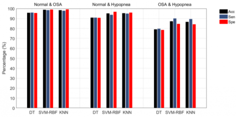
Figure 9. Performance of proposed system using various classifiers and under (one-vs-one) classification method
The indices DispEnVLF, DispEnLF, DispEnHF, DispEnTotal, DispEnLF/HF, DispEnpVLF, DispEnpLF, and DispEnpHF in the three time scales small (1 to 5), medium (6 to 10) and large (11 to 20) are thought to be the most statistically significant to discriminate the normal and OSA episodes, the normal and hypopnea episodes, according to the p-value of the t-test.
The indices DispEnVLF, DispEnLF, DispEnHF, DispEnTotal, DispEnLF/HF, DispEnpVLF, DispEnpLF, and DispEnpHF in the medium (6 to 10) time scales are thought to be the most statistically significant indices to discriminate the OSA and hypopnea episodes, according to the p-value of the t-test.
The normal and OSA episodes, the normal and hypopnea episodes, and the OSA and hypopnea episodes were categorized using the DT, SVM-RBF, and KNN classification techniques, respectively. Table 2 and Figure 9 compare the accuracy, specificity, and sensitivity of several categorization techniques across different episodes. Table 2 and Figure 9 demonstrate that SVM-RBF has the best accuracy and specificity for normal and OSA episodes, normal and hypopnea episodes, and OSA and hypopnea episodes, with 98.58% and 98.34%, 95.69% and 94.74%, 87.04% and 89.96%, respectively.
The normal, OSA and hypopnea episodes were also graded using multi-classification method to further assess the ability of the proposed method for the SAHS recognition. The three sample groups were examined using the DT, SVM-RBF, and KNN classifiers, and the accuracy, specificity, and sensitivity are shown in Table 3 and Figure 10. From the results, it can be seen that by combining the indices of the small (1 to 5) medium (6 to 10) and large (11 to 20) time scales in the case of SVM-RBF, we achieved the highest mean for accuracy, specificity and sensitivity being 93.94%, 96.92% and 93.91% over straight.
Figure 11 also shows the true positive (TP) and false positive (FP) rates for all classifiers, including DT, SVM-RBF, and KNN, for each class. As shown in Figure 8, the maximum likelihood of normal episodes (predict class) being classified as normal episodes (true class) is 98.01% (SVM-RBF), and the samples are classified into OSA and hypopnea episodes (true class) with a minimum likelihood of 0.17% and 1.82% (SVM-RBF), respectively. The probability of OSA episodes (predicted class) being maximum categorized as OSA episodes (true class) is 93.33% (KNN). The OSA episodes (predicted class) are more likely to be categorized incorrectly as hypopnea episodes (true class) (DT: 17.08%, SVM-RBF: 7.46%, KNN: 6.80%). The probability of hypopnea episodes (predicted class) being maximum categorized as hypopnea episodes (true class) is 86.10% (SVM-RBF).
Table 3. Performance of proposed system using various classifiers and under (one-vs-all) classification method
|
Object |
Mean Scales |
DT |
SVM-RBF |
KNN |
||||||
|
Acc (%) |
Spe (%) |
Sen (%) |
Acc (%) |
Spe (%) |
Sen (%) |
Acc (%) |
Spe (%) |
Sen (%) |
||
|
Normal |
1 to 5 |
92.8571 |
95.7916 |
90.5473 |
95.8478 |
97.6308 |
91.8740 |
94.4257 |
96.7000 |
92.7032 |
|
OSA |
82.3328 |
90.8444 |
79.6020 |
83.9316 |
91.7976 |
81.4262 |
81.9398 |
90.5594 |
81.2604 |
|
|
Hypopnea |
74.6082 |
86.3636 |
78.9386 |
77.0898 |
87.5943 |
82.5871 |
77.0598 |
88.0772 |
79.1045 |
|
|
mean |
83.2660 |
90.9999 |
83.0293 |
85.6231 |
92.3409 |
85.2957 |
84.4751 |
91.7789 |
84.3560 |
|
|
Normal |
6 to 10 |
88.0342 |
92.8571 |
85.4063 |
88.9621 |
93.3267 |
89.5522 |
85.4430 |
90.8640 |
89.5522 |
|
OSA |
78.3694 |
88.0074 |
78.1095 |
82.0380 |
90.5967 |
78.7728 |
80.7047 |
89.4399 |
79.7678 |
|
|
Hypopnea |
70.4655 |
84.2735 |
72.8027 |
74.1573 |
86.3095 |
76.6169 |
74.6988 |
87.4144 |
71.9735 |
|
|
mean |
78.9564 |
88.3793 |
78.7728 |
81.7191 |
90.0777 |
81.6473 |
80.2822 |
89.2394 |
80.4312 |
|
|
Normal |
11 to 20 |
86.5646 |
91.6842 |
84.4113 |
90.2896 |
94.0126 |
87.8939 |
86.2069 |
91.1672 |
87.0647 |
|
OSA |
75.8621 |
85.3333 |
80.2653 |
76.8740 |
86.6728 |
79.9337 |
75.1166 |
85.0327 |
80.0995 |
|
|
Hypopnea |
66.3808 |
83.5156 |
64.1791 |
69.4118 |
84.7571 |
68.4909 |
68.9408 |
85.3514 |
63.6816 |
|
|
mean |
76.2692 |
86.8444 |
76.2852 |
78.8585 |
88.4808 |
78.7728 |
76.7548 |
87.1838 |
76.9486 |
|
|
Normal |
All |
93.4211 |
96.1014 |
94.1957 |
98.9950 |
99.4614 |
98.0100 |
97.8188 |
98.8095 |
96.6833 |
|
OSA |
86.4111 |
93.1338 |
82.2554 |
92.0661 |
95.9664 |
92.3715 |
88.0691 |
93.5429 |
93.0348 |
|
|
Hypopnea |
78.1499 |
88.5928 |
81.2604 |
90.7743 |
95.3488 |
91.3765 |
89.9306 |
95.1747 |
85.9038 |
|
|
mean |
85.9940 |
92.6093 |
85.9038 |
93.9451 |
96.9255 |
93.9193 |
91.9395 |
95.8424 |
91.8740 |
|
Figure 10. Performance of proposed system using various classifiers and under (one-vs-all) classification method
Figure 11. The TPR and FPR at different classifier (a) KNN; (b) SVM; (c) DT
The present paper describes a new method for detecting and classifying episodes of obstructive sleep apnea and hypopnea using ECG signal. This method is based on extracting the calculated the mean of the small (1 to 5), medium (6 to 10) and large (11 to 20) time scales of the multiscale dispersion entropy (MDE) directly from the VLF, LF, HF and TP sub-band signals. So that the VLF, LF and HF sub-band signals were obtained by analyzing the HRV signal using CWT followed by ICWT technique. The CWT enables for signal analysis at multiple scales and translations according to the problem (It allows extracting each band between specific frequency bands). The ICWT approach aided us in noise reduction, to be implemented in the wavelet domain and in the signal reconstruction that resulted after processing.
Figures 4-9 and Figure 10 represent the mean and standard deviation of the indices based on the method of calculating the MDE in the small (1 to 5), medium (6 to 10) and large (11 to 20) time scales of the sub-band signals. As can be shown, the DispEnLF and DispEnLF/HF indices indicate a rising tendency among normal, hypopnea, and OSA episodes. Between normal, hypopnea, and OSA episodes, the DispEnHF and DispEnpHF indices indicate a declining tendency. In the normal, hypopnea, and OSA episodes, the ShEnVLF and ShEnpVLF indices exhibit volatility in the three time scales of MDE.
Because LF is associated with sympathetic nervous system activity, variations in HRV's LF sub-band signal change significantly in the sympathetic nervous system. HF is thought on the other hand to be associated with parasympathic activity. The physiological meaning of the very low frequency factor (VLF) is still unclear, however, and was merely determined using long-term rhythms [37]. Because typical people's parasympathetic activity increases during nighttime sleep, the fluctuation patterns of the HRV increase inside the HF band, the texture of the HF sub-image of CWT and sub-signal of ICWT is complicated. The sympathetic activity inhibiting HF component diminishes by comparison, i.e. in normal episodes, the fluctuations of HRV decreases with LF band, thereby simplifying the texture of the CWT sub-band image and ICWT sub-band signal of LF. Parasympathetic activity is, however, inhibited for OSA patients due to predominant sympathetic activity. Thus, the oscillation features of the HRV are reduced in the HF band, while the range of LF is increased in comparison to ordinary episodes. As a consequence, the DispEnLF and DispEnLF/HF indices show an increasing trend between the normal, hypopnea and OSA episodes, while the DispEnHF and DispEnpHF indices show a decreasing trend between the normal, hypopnea and OSA episodes in both three time scales: small, medium and large. As the variation of HRV signals from normal to hypopnea and normal to hypopnea episodes was represented largely in the HF band and the LF bands, there were therefore substantial disparities in both normal and hypopnea or OSA episode, and there was no significant difference between OSA and a hypopnea episode.
As you know from Table 2 and Figure 9, the highest classification accuracy between the normal and OSA episodes is 98.58% using SVM classifier with Radial Basis Function (RBF) kernel and combination indices of the small, medium and large time scales. Because OSA causes breathing disorders during sleep and increases sympathetic nervous system activity, it's simpler to discriminate between the two types of normal and OSA episodes. In OSA episodes and hypopneas, the HRV signal has more turbulent vibrational properties, whereas the HRV signal in a healthy individual has more regular and tuned qualities. This difference can be seen by the distribution of the wavelet spectral power in the time-frequency domain of HRV signal. The accuracy for both normal and hypopnea episodes is 95.69% using the SVM-RBF classifier and the combination of the indices of the small, medium and large time scales, which is lower than the normal and OSA episodes due to the diminution turbulent vibrational properties of the HRV signal in the hypopnea episodes.
The accuracy between the OSA and the hypopnea is 87.04%, by means of the SVM-RBF classifier and combining small, medium and large time scales, which is less than in the previous two examples. The fluctuating features of the HRV signal shows some parallels between OSA and hypopnea episodes. The activity of the sympathetic nervous system, which may produce OSA episodes, is more important than the activity of the hypoventilation episodes, resulting a difference between the two OSA and hypopnea episodes.
The average classification accuracy of three episodes (normal, OSA, and dyspnea) in Table 3 and Figure 10 is 93.94% by using the multi-classification technique of SVM-RBF classifier and combining small, medium and large time scale indices. The decrease in accuracy is due to the increasing types of categorization, which increases the probability of categorizing data into similar groups.
Several classification tests were performed in the proposed study, with the three-category ECG dataset (normal episodes, OSA episodes and hypopnea) so that the most difficult to accurately classify were OSA episodes and hypopnea. The traditional OSA detection and classification approach is based on the use of HRV and EDR signals analysis using time and frequency domains either alone or in combination. Khandoker et al. [13] demonstrated the best results for identifying OSA using the classic OSA detection and classification approach, which uses time-frequency domain analysis and an ANN classifier. They were able to detect apnea episodes with 94.84% accuracy which is less than that obtained by our proposed method. In reality, exploiting temporal characteristics of signal in real-time applications might be beneficial since they are simple to extract and provide a low-complexity calculation. However, in order to meet the established criteria, they have to split the original signal into short (5 sec) segments. Splitting the signal into small pieces often leads to loss and spoilage of the general dynamics of the signal. Also, there is no mathematical equation that can be used to determine the threshold levels in order to separate the sudden rises from the noise. Furthermore, ECG signal is a sort of weak and unstable signal that is readily impacted by noise, and frequency band analysis is not a solution since the signal is not stable.
As a result, we concentrated our efforts in this study on the HRV signal, which may be utilized as markers of cardio-respiratory rhythm coordination during SAHS, and we sought to uncover their non-linear features like multiscale dispersion entropy. Other research that used the same database (the Apnea-ECG database) for training and testing were compared to the suggested automated OSA detection methodology. Chazal et al. [10] and McNames and Frazer [38] are both achieving highly accurate. The authors [10] utilized a high-dimensional feature matrix (128 features), which results in a complicated technique. Furthermore, fundamental flaw is that their classification processes are not automated [38]. Also, in the classification stage, they deleted borderline recordings (10 participants), which is not the case in our classification work. Varon et al. [39] and Bali et al. [40] achieved the best results (100% accuracy) among the approaches for automated OSA identification. The methods mentioned in the studies [17-18] derived different characteristics from the RR intervals and EDR signal with an accuracy of 85.26 percent and 82.07 percent, respectively. Furthermore, several other researches, such as [19, 38], have rejected some of the noisy recordings with poor data quality in the process. As a result of the noisy nature of physiological signals, these techniques require high-quality datasets, which are not readily available.
In summary, the study's novelty stems mostly from the use of multiscale entropy characteristics of the HF, LF, VLF and TP sub-band signals in SAHS detection. The 24 novel indices in this article allow OSA and hypopnea to be recognized. Furthermore, this article benefits from the fact that the OSA and hypopnea episode may be recognised just with 5 minutes of the ECG signal, and that SAHS can be screened by the OSA episode, but also the hypopnea episode. There are few studies to differentiate obstructive sleep apnea episodes from episodes of hypopnea. As a result of this research, the suggested new indices based on CWT and MDE can differentiate between OSA episodes and hypopnea episodes, and these indices perform well - Accuracy, Sensitivity, and Specificity, respectively, are 89.87%, 87.13%, and 92.86%.
In this work, twenty-four novel CWT and MDE based indices are suggested for SAHS identification, which are accomplished by evaluating the HRV signal. The indices are extracted by the small, medium and large time scales of the MDE method. In the proposed method, firstly, the power spectrum of HRV is estimated by the CWT method, then, TP, HF, LF, and VLF sub-band signals is obtained by using the ICWT technique. Finally, the vibrational characteristics of HRV signals are assessed, and SAHS identification is accomplished by computing the mean of the MDE values for each sub-band signal over three time scales: small (1 to 5), medium (6 to 10) and large (11 to 20) and their relationships between them. The recordings from the Physionet Apnea–ECG database and the UCD database were utilized to test the performance of the CWT and MDE based indices, and each HRV segment was categorized using the DT, SVM-RBF, and KNN classification techniques. For SAHS recognition, the SVM-RBF classification technique had the highest accuracy, with an average of 93.94%, an average sensitivity of 93.91, and an average specificity of 96.92%. It cannot be denied that the CWT and MDE-based indices proposed in this article offer a new step for SAHS detection. In the future, we can support the proposed method with other nonlinear properties, such as fuzzy and permutaion entropy, can be used to improve the suggested technique further.
[1] Liu, Y.T., Zhang, H.X., Li, H.J., Chen, T., Huang, Y.Q., Zhang, L. (2018). Aberrant interhemispheric connectivity in obstructive sleep apnea-hypopnea syndrome. Frontiers in Neurology, 9: 314. https://doi.org/10.3389/fneur.2018.00314
[2] Duarte, R.L.M., Mello, F.C.Q., Magalhães-da-Silveira, F.J., Oliveira-e-Sá, T.S., Rabahi, M.F., Gozal, D. (2015). Withstanding the obstructive sleep apnea syndrome at the expense of arousal instability, altered cerebral autoregulation and neurocognitive decline. Journal of Integrative Neuroscience, 14(2): 169-193. https://doi.org/10.1142/S0219635215500144
[3] Malhotra, A., White, D.P. (2002). Obstructive sleep apnoea. Lancet, 360(9328): 237-245. https://doi.org/10.1016/S0140-6736(02)09464-3
[4] Tobal, G.G.C., Álvarez, A.M.L., Álvarez, D., Del Campo, F., Santos, T.J., Hornero, R. (2015). Diagnosis of pediatric obstructive sleep apnea: Preliminary findings using automatic analysis of airflow and oximetry recordings obtained at patients’ home. Biomedical Signal Processing and Control, 18: 401-407. https://doi.org/10.1016/j.bspc.2015.02.014
[5] Hudgel, D.W. (2016). Sleep apnea severity classification -revisited. Sleep, 39(5): 1165-1166.
[6] Berry, R.B., Budhiraja, R., Gottlieb, D.J., et al. (2012). Rules for Scoring Respiratory Events in Sleep: Update of the 2007 AASM Manual for the Scoring of Sleep and Associated Events. Journal of Clinical Sleep Medicine, 8(5): 597-619. https://doi.org/10.5664/jcsm.2172
[7] Deutsch, P.A., Simmons, M.S., Wallace, J.M. (2006). Cost-effectiveness of split-night polysomnography and home studies in the evaluation of obstructive sleep apnea syndrome. Journal of Clinical Sleep Medicine, 2(2): 145-153. https://doi.org/10.5664/jcsm.26508
[8] Penzel, T., Moody, G.B., Mark, R.G., Goldberger, A.L., Peter, J.H. (2000). The apnea-ECG database. In Computers in Cardiology 2000, 27: 255-258. https://doi.org/10.1109/CIC.2000.898505
[9] Guilleminault, C., Winkle, R., Connolly, S., Melvin, K., Tilkian, A. (1984). Cyclical variation of the heart rate in sleep apnoea syndrome: Mechanisms, and usefulness of 24 h electrocardiography as a screening technique. The Lancet, 323(8369): 126-131. https://doi.org/10.1016/S0140-6736(84)90062-X
[10] de Chazal, P., Heneghan, C., Sheridan, E., Reilly, R., Nolan, P., O’Malley, M. (2000). Automatic classification of sleep apnea epochs using the electrocardiogram. Computers in Cardiology, 27: 745-748. https://doi.org/10.1109/CIC.2000.898632
[11] de Chazal, P., Heneghan, C., Sheridan, E., Reilly, R., Nolan, P., O’Malley, M. (2003). Automated processing of the single-lead electrocardiogram for the detection of obstructive sleep apnoea. IEEE Transactions on Biomedical Engineering, 50(6): 686-696. https://doi.org/10.1109/TBME.2003.812203
[12] Hossen, A., Ghunaimi, B.A., Hassan, M.O. (2005). Subband decomposition soft decision algorithm for heart rate variability analysis in patients with obstructive sleep apnea and normal controls. Signal Process, 85(1): 95-106. https://doi.org/10.1016/j.sigpro.2004.09.004
[13] Khandoker, A.H., Gubbi, J., Palaniswami, M. (2009). Automated scoring of obstructive sleep apnea and hypopnea events using short-term electrocardiogram recordings. IEEE Transactions on Information Technology in Biomedicine, 13(6): 1057-1067. https://doi.org/10.1109/TITB.2009.2031639
[14] Mendez, M.O., Corthout, J., Van Huffel, S., Matteucci, M., Penzel, T., Cerutti, S. (2010). Automatic screening of obstructive sleep apnea from the ECG based on empirical mode decomposition and wavelet analysis. Physiological Measurement, 31: 273-289. https://doi.org/10.1088/0967-3334/31/3/001
[15] Bsoul, M., Minn, H., Tamil, L. (2011). Apnea MedAssist: Real-time sleep apnea monitor using single-lead ECG. IEEE Transactions on Information Technology in Biomedicine, 15: 416-427. https://doi.org/10.1109/TITB.2010.2087386
[16] Nguyen, H.D., Brek, A.W., Cheng, Q., Bruce, A.B. (2014). An online sleep apnea detection method based on recurrence quantification analysis. IEEE Journal of Biomedical and Health Informatics, 18: 1285-1293. https://doi.org/10.1109/JBHI.2013.2292928
[17] Atri, R., Mohebbi, M. (2015). Obstructive sleep apnea detection using spectrum and bispectrum analysis of single-lead ECG signal. Physiological Measurement, 36: 1963-1980. https://doi.org/10.1088/0967-3334/36/9/1963
[18] Janbakhshi, P., Shamsollahi, M.B. (2018). Sleep apnea detection from single-lead ECG using features based on ECG-Derived respiration (EDR) signals. IRBM, 39: 206-218. https://doi.org/10.1016/j.irbm.2018.03.002
[19] Li, Y., Pan, W., Jiang, Q., Li, K. (2019). Sliding trend fuzzy approximate entropy as a novel descriptor of heart rate variability in obstructive sleep apnea. IEEE Journal of Biomedical Health Informatics, 23: 175-183. https://doi.org/10.1109/JBHI.2018.2790968
[20] Feng, K., Qin, H., Wu, S., Pan, W., Liu, G. (2020). A sleep apnea detection method based on unsupervised feature learning and single-lead electrocardiogram. IEEE Transactions on Instrumentation and Measurement, 70: 1-12. https://doi.org/10.1109/TIM.2020.3017246
[21] Xie, B., Qiu, W., Minn, H., Tamil, L., Nourani, M. (2011). An improved approach for real-time detection of sleep apnea. Proceedings of International Conference on Bio-inspired Systems and Signal Processing, Rome, Italy, January 26-29.
[22] St. Vincent’s University Hospital/University College Dublin Sleep ApneaDatabase. (2008). Available: http://www.physionet.org/pn3/ucddb.
[23] Bouaziz, F., Boutana, D., Benidir, M. (2012). Automatic detection method of R-wave positions in electrocardiographic signals. The 24th International Conference on Microelectronics, Algiers, pp. 1-4. https://doi.org/10.1109/ICM.2012.6471429
[24] Martis, R.J., Acharya, U.R., Min, L.C. (2013). ECG beat classification using PCA, LDA, ICA and discrete wavelet transform. Biomedical Signal Processing and Control, 8: 437-448. https://doi.org/10.1016/j.bspc.2013.01.005
[25] Pan, J., Tompkins, W.J. (1985). A real-time QRS detection algorithm. IEEE Transactions on Biomedical Engineering, 8: 230-236. https://doi.org/10.1109/TBME.1985.325532
[26] Wang, T., Lu, C., Sun, Y., Yang, M., Liu, C., Ou, C. (2021). Automatic ECG classification using continuous wavelet transform and convolutional neural network. Entropy, 23: 119-132. https://doi.org/10.3390/e23010119
[27] Wu, Z., Lan, T., Yang, C., Nie, Z. (2019). A novel method to detect multiple arrhythmias based on time-frequency analysis and convolutional neural networks. IEEE Access, 7: 170820-170830. https://doi.org/10.1109/ACCESS.2019.2956050
[28] Rostaghi, M., Azami, H. (2016). Dispersion entropy: A measure for time-series analysis. IEEE Signal Process Letters, 23: 610-614. https://doi.org/10.1109/LSP.2016.2542881
[29] Zheng, J., Pan, H., Liu, Q., Ding, K. (2020). Refined time-shift multiscale normalised dispersion entropy and its application to fault diagnosis of rolling bearing. Physica A: Statistical Mechanics and its Applications, 545: 123641. https://doi.org/10.1016/j.physa.2019.123641
[30] Azami, H., Rostaghi, M., Abasolo, D., Escudero, J. (2017). Refined composite multiscale dispersion entropy and its application to biomedical signals. IEEE Transactions on Biomedical Engineering, 64(12): 2872-2879. https://doi.org/10.1109/TBME.2017.2679136
[31] Azami, H., Escudero, J. (2018). Coarse-graining approaches in univariate multiscale sample and dispersion entropy. Entropy, 20(2): 138. https://doi.org/10.3390/e20020138
[32] Cartas-Rosado, R., Becerra-Luna, B., Martínez-Memije, R., Infante-Vázquez, O., Lerma, C., Pérez-Grovas, H. (2020). Continuous wavelet transform based processing for estimating the power spectrum content of heart rate variability during hemodiafiltration. Biomed Signal Process Control, 62: 102031. https://doi.org/10.1016/j.bspc.2020.102031
[33] Acharya, U.R., Sudarshan, V.K., Ghista, D.N., Eugene, L.W.J. (2015). Computer-aided diagnosis of diabetic subjects by heart rate variability signals using discrete wavelet transform method. Knowledge-Based Systems, 81: 56-64. https://doi.org/10.1016/j.knosys.2015.02.005
[34] Acharya, U.R., Fujita, H., Bhat, S., Raghavendra, U., Gudigar, A., Molinari, F., Vijayanathan, A., Ng, K.H. (2016). Decision support system for fatty liver disease using GIST descriptors extracted from ultrasound images. Information Fusion, 29: 32-39. https://doi.org/10.1016/j.inffus.2015.09.006
[35] Sharma, R., Pachori, R.B., Acharya, U.R. (2015). An integrated index for the identification of focal electroencephalogram signals using discrete wavelet transform and entropy measures. Entropy, 17: 5218-5240. https://doi.org/10.3390/e17085218
[36] Suykens, J.A.K., Vandewalle, J. (1999). Least squares support vector machine classifiers. Neural Process Letters, 9: 293-300. https://doi.org/10.1023/A:1018628609742
[37] Sztajzel, J. (2004). Heart rate variability: A noninvasive electrocardiographic method to measure the autonomic nervous system. Swiss Medical Weekly, 134: 514-522.
[38] McNames, J.N., Fraser, A.M. (2000). Obstructive sleep apnea classification based on spectrogram patterns in the electro-cardiogram. Computers in Cardiology, 27: 749-752. https://doi.org/10.1109/CIC.2000.898633
[39] Varon, C., Caicedo, A., Testelmans, D., Buyse, B., Van Huffel, S. (2015). A novel algorithm for the automatic detection of sleep apnea from single-lead ECG. IEEE Transactions on Biomedical Engineering, 62(9): 2269-2278. https://doi.org/10.1109/TBME.2015.2422378
[40] Bali, J., Nandi, A., Hiremath, P.S. (2020). Efficient ANN algorithms for sleep apnea detection using transform methods. In Advancement of Machine Intelligence in Interactive Medical Image Analysis, 99-152. https://doi.org/10.1007/978-981-15-1100-4_5