Angelin Preethi Rajakumar* | Anandharaj Ganesan
© 2022 IIETA. This article is published by IIETA and is licensed under the CC BY 4.0 license (http://creativecommons.org/licenses/by/4.0/).
OPEN ACCESS
The growth of serial remote sensing images (SRSI) offers abundant information for determining sequential spatial patterns in several fields like vegetation cover, urban development, and agricultural monitoring. Or else, traditional sequential pattern-mining algorithms cannot be applied efficiently or directly to remote sensing images. Here a new technique is proposed for enhancing the mining efficacy of spatial sequential patterns from raster serial remote sensing images (SRSI) based on pixel grouping approach. The modified extrema pattern is employed to offering grey-scale invariant transform of intensity values unlike previously employed local ternary pattern. The pattern features are computed by transformation process from which the multilinear matrix decomposition of the image is made by computing the covariance estimation on recognizing their orthogonal component. The matrix decomposition is then attained based on run length encoding process (RLC). The two rows of RLC vectors are intersected to attain pixel group matrix. Finally, the compressed image is attained in an efficient manner with effective mining time. The performance outcome reveals that the technique offered in this paper is capable of extracting spatial sequential patterns from SRSI effectively. The proposed system ensures that the entire patterns are extracted at a lower time consumption when compared to the state-of-the-art technologies.
serial remote sensing images, pixel grouping, modified extrema pattern, multilinear matrix decomposition, run length encoding
Recently, the researchers all over the world have concentrated on the image classification of image which is considered as a significant technology in case of pattern recognition and computer vision. Generally, Satellite images are in the digital form. An image processing technique can be employed for retrieving the exact set of data from the images that are stored. Thus, this process can be helpful in enhancing the visual perception and for modifying or repairing the image that is based on image blurring, deformation of image, or detoriation of an image. There were some techniques that are available for analyzing image and they rely on the specific issue’s necessities [1-4]. The algorithms of image classification and segmentation are employed in several image regions in the thematic groups [5-8]. The image classification forms can be categorized as four groups in different angles like image clustering based on model-driven, edge-based, and region. Due to this simple principle like strong and quick classification effect, CNN is employed widely. Moreover, the images are classified normally by means of a single CNN [9-12], it is probable for getting stuck in local maximum, the blurring of boundaries occurs with bad visual effect [13, 14].
The foremost issues are not only image capturing however also to process the information captured fast and disseminate them in an instant manner at the specified target detection and tehri classification is estimated by their accuracy. The primary method for any problem related to the detection of target is to isolate various components of the scene and recognize the one which is of interesting one from the remaining. Still, the classification approach is a complex task and a valid issue for detecting the robust satellite target system. There will be some issues in identifying the clutter and guard’s region. Henceforth there is a need to address the issues of satellite image classification by means of an effective system.
1.1 Motivation and objective of proposed scheme
Serval existing techniques have been presented for mining SRSI. However, there were limitations like the method is not effective for multilinear component and so on. So as to overcome this shortcoming, this method is proposed with the use of modified extrema pattern to provide grey-scale invariant transform. The multilinear matrix decomposition is employed instead of singular value decomposition process as it is not applicable for multilinear data. The run length encoding based pixel grouping is presented and the image is compressed in an effective manner.
1.2 Organization
The remaining portion of this manuscript is schematized as shown: section II is the depiction of various existing technique’s review employed so far. Section III is the detailed explanation of proposed methodology. The performance analysis of the proposed system is depicted in section IV. Finally, the conclusion of proposed system is made clear in section V.
A method of pixel clustering-dependent one for enhancing the spatial sequential mining from raster SRSI was presented [15]. Initially, the images are compressed through the run-length coding scheme. After that, the pixels having undistinguishable sequences are clustered by means of run-length code dependent overlay function. At last, the pruning scheme was presented for extending the prefix span scheme for skipping unwanted database scanning on mining the group of pixels. The experimental outcomes reveal that the presented method is capable of extracting the spatial sequential patterns in an effective manner.
A scheme of resilient distributed datasets (RDD) was offered in this [16] work, which is meant for processing the remote sensing image, and in turn employs three significant kinds of mosaicking image that covers region estimation of overlapping that are the type of transformation functions of self-defined RDD. This is the one at which the extending functionality is attained in spark. At last, the parallel processing of an image mosaicking is then realized through performing the self-defined RDD operators along with the conversion implicit.
The application of high-resolution network (HRnet) was presented in the study of Zhang et al. [17] for producing the features of high-resolution deprived of the decoding step. However, low-to-high features were being extracted from various branches in a separate manner for strengthening the scale-oriented strengthening of contextual data. The features having low-resolution has more semantic information and consists of minor spatial size. Hence, they were employed for modelling the long-term spatial correlations. The branches with high-resolution were implemented on introducing the adaptive spatial pooling (ASP) unit for the aggregation of more contexts that are local. On combining those designs of aggregation context over various levels, the architecture attained is capable of employing spatial context at local and also at global level.
In this approach [18], the author contributed the issue on enhancing the representation of features in two different manners. In one hand, the patch attention module (PAM) was employed for enhancing the context information embedding depending on the patch wise computation of local attention. In other hand, the attention embedding module (AEM) was presented for enriching the semantic information of lower-level features on embedding the features of higher level. These two modules were light weight and could be employed for processing the features extracted by convolutional neural networks (CNNs).
The process of ultimate research well-defined as the quantization dependent retrieval of images was offered which is termed as hypergraph and the process of hacking [19]. Song et al. [20] employed generative encoders, and the multimodal stochastic recurrent neural network (RNNs) for an efficient recovery of images, hierarchical binary auto-encoders.
An efficient unsupervised method of evaluation was presented in the study of Gao et al. [21] for measuring the segmentation outcome quality in a quantitively manner for overcome this issue. In this technique, spatial features and multiple spectral of images were extracted initially in a simultaneous manner and then combining them into feature set for enhancing the feature representation quality of the ground objects [22]. The indicators presented for spatial autocorrelation and spatial graded heterogeneousness were encompassed for estimating the segmentation properties at this feature set that were integrated.
A simple and reliable binary logic regression solution was presented [23] for the classification of image. The review was conducted in India’s subtropical east coast region that was surrounded by means of fallow land, land, and the water bodies. Diverse habits of categorizing objects through employing several techniques of image processing the setting of remote sensing was presented [4]. The probability of calculation was suggested for all pixels in a class [24]. The values were related and the class the pixels were assigned at which the probability is high. This is an effective technique highly for the purpose of classifying satellite images, specifically the images of multi-spectral properties. However, this technique needs a high time for computation. The sparse SVM classifier algorithm was introduced by Menaka et al. [25]. The images that are segmented were classified as small patches. Then after the extraction process, the images segmented will be classified as small patch [26, 27]. The image patches and sparse images are employed after the extraction mechanism. The sparse image is the resolved by verifying the pixels of image and is optimized for the efficiency of classification.
The classification of Remote sensing image is a usual application of remote sensing images [28]. So as to enhance the remote sensing image classifier performance, combinations of multiple classifiers were employed for categorizing the images of Landsat-8 Operational Land Imager (Landsat-8 OLI). Some classifier combination algorithms and techniques were examined. The collaborative classifier comprising of five classifiers member is made. The outcomes of each classifier member were assessed. The strategy of voting is investigated to integrate the classification outcomes of classifier member. The outcomes illustrates that the classifiers entirely have dissimilar concerts and the combination of multiple classifiers delivers improved concert on comparing the single classifier, and attains overall higher classification accuracy.
Research was carried on [29] regarding multiple-feature flexible hashing learning context meant for LSRSIR that took multiple features that were complementary as the input and in turn learns the feature mapping function hybrid strategy that projects the multiple features of remote sensing images to the representation of low-dimensional binary features [30]. Additionally, the compressed representations of feature could be utilized directly in LSRSIR with the assistance of the hamming distance measured. So as to illustrate the presented hashing learning multiple feature process superiority, the presented approach was compared with traditional techniques for the two-publicly available datasets alike large-scale remote sensing image datasets.
The long-term sequence Landsat summer images was employed in 2002-2019 for investigating the vegetation growth status variation and their effects of ecological restoration [31]. Consistent with the explicit study area situation, the calculated GRNDVI (Green-Red Normalized Difference Vegetation Index) from the data of remote sensing was employed for analyzing the mine vegetation growth and the changes in annual growth. The outcomes reveal that the technique could accurately access the growth of vegetation trend in the area of review. A quantized ternary pattern-based pixel grouping and singular value decomposition-Run length coding-based pattern mining was employed in the study of Preethi and Anandharaj [32]. The presented algorithm is effective in terms of mining time and the generation of sequence pattern.
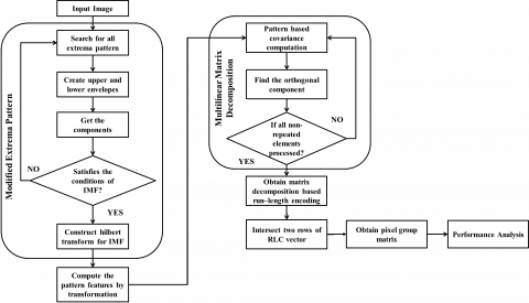
The detailed explanation of the proposed workflow is given in this section. Usually, the satellite remote sensing image are of higher bandwidth which is not efficient for further processing. Hence, this will be converted to another form termed sequential pattern mining. In sequential pattern mining process, relevant patterns are converted to sequential forms from the image patterns. The overall flow of the presented approach is shown in Figure 1 provided below.
3.1 Modified Extrema pattern for pixel grouping
On converting the image into patterns, the greyscale transformation is formed which is represented in intensity wise at which the modified extrema pattern is employed for grouping the image in pixel wise manner as a block. The minimum and maximum extrema values in each block are considered for forming sequence. Thus, the pattern formation is done by taking maximum extrema values.
Local extrema patterns typically relate the center pixel and the neighborhood reference pixel on comparing the level of intensity. This extrema pattern is presented by Murala and this is regarded as the Local Binary pattern (LBP) continuation in such a manner, this could deal with the information regarding edges in various positions. This in turn relates the pixels in 01, 451, 901, and 1351 positions in terms of center pixel and in turn assigns 1 once both neighboring pixels were in the specific position, whichever less or greater distinctly on comparing center pixel, then in the similar way it allocates 0 in case, one pixel is greater than center pixel. On behalf of center pixel Ic and the equivalent neighbor pixel Ii, LEP is computed as shown below:
$I_{i}^{\prime}=I_{i}-I_{c}$ (1)
where, i=1, 2...,8.
$I_{i}^{\prime}(\varphi)=P_{3}\left(I_{k}^{\prime} I_{k+4}^{\prime}\right)$ (2)
where, k=(1+ψ/45), $\forall \varphi=0^{0}, 45^{0}, 90^{0}, 135^{0}$.
$P_{3}\left(I_{k}^{\prime} I_{k+4}^{\prime}\right)= \begin{cases}1 & I_{k}^{\prime} \times I_{k+4}^{\prime} \geq 0 \\ 0 & \text { Else }\end{cases}$ (3)
$\operatorname{LEP}\left(I_{c}\right)=\sum_{\varphi} 2^{\varphi / 45} \times I_{k}^{\prime}(\varphi)$ (4)
where, $\forall \varphi=0^{0}, 45^{\circ}, 90^{\circ}, 135^{\circ}$.
$H(L) \mid L E P=\sum_{m=1}^{M} \sum_{n=1}^{N} P_{2}(L E P(m, n), L)$ (5)
where, $L \in[0,15]$.
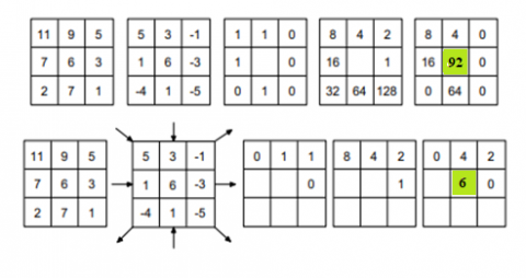
Typically, LEPs were computed by means of above two Eqns. (4) and (5), at which the angle of LEP computation is represented by ψ and in Eq. (5), the local extrema pattern histogram is being generated. A window of 3×3 matrix illustration of both LEP and LBP was illustrated Figure 2. In Figure 2, the matric of 3×3 is considered for explanation and each pixel boundary is being subtracted from the center pixel values.
The pattern of LBP is attained and this pattern is then multiplied by means of weights, summed up for the value of local binary pattern as shown in the upper part of the Figure 2. Likewise, in LEP similar window 3×3 is selected, and the neighboring pixels are then subtracted from the value of center pixel as shown in the second lower part of Figure 2. In the calculation of LEP pattern, for positive and negative value representation inside and outside arrow was shown correspondingly. In case, both arrows were different one will be inside one and the other in outside one at some specific location i.e., $0^{0}, 45^{\circ}, 90^{\circ}, 135^{\circ}$, then the pattern value is ‘0’, and in case both arrows were same the pattern value is ‘1’ at that direction.
Figure 1. Flow of the proposed system
Figure 2. Illustration of LEP and LBP example
At this time, the attained four vales were multiplied by means of weight and the values of LEP were attained. The wavelet Hilbert transform offers the input data decomposition process thereby removing the components of high-frequency. These high-frequency components were termed as Intrinsic Mode Function (IMF). This process will be repeated till the following condition is satisfied.
|
Algorithm 1: Modified Extrema Pattern |
|
Input: Input image $I_{i n p}$ Output: Extreme pattern result $E x t r_{\text {pat }}$ |
|
Step 1: Estimate the difference between center pixel and adjacent pixels of each pattern for $i=1: 3: I_{i n p}^{r o w}$ for $j=1: 3: I_{i n p}^{c o l}$ $I_{i n p}^{m}=I_{i n p}[\mathrm{i}$ to $\mathrm{i}+3, \mathrm{j}$ to $\mathrm{j}+3]$ $I_{i n p}^{m}{ }^{\prime}=I_{i n p}^{m}- I_{i n p}^{c} \quad m=1,2, \ldots, 8$ End for End for $I_{i n p}^{\text {row }}-$ number of rows of $I_{i n p}$ $I_{i n p}^{c o l}-$ number of columns of $I_{i n p}$ Step 2: Binary pattern conversion with respect to center pixel based on the upper and lower envelops, $I_{i n p}^{m}(\rho)=F_{n}\left(I_{i n p}^{m}, I_{i n p}^{m+4^{\prime}}\right) \rho=0^{\circ}, 45^{\circ}, 90^{\circ}$ and $135^{\circ}$ $F_{n}\left(I_{i n p}^{m}{ }^{\prime}, I_{i n p}^{m+4^{\prime}}\right)=\left\{\begin{array}{lc}1 & I_{i n p}^{m}{ }^{\prime} \oplus I_{i n p}^{m+4^{\prime}} \\ 0 & \text { else }\end{array}\right.$ Step 3: Form the extrema pattern at center pixel with intrinsic mode function, $\operatorname{Extr}_{\text {pat }}\left(I_{i n p}^{c}\right)=\sum I_{i n p}^{m}(\rho) * 2^{\rho / 45}$ Step 4: Perform Hilbert transform for histogram of that pattern, ${{H}_{Ext{{r}_{pat}}}}=hilbert\left\{ \sum\limits_{r=1}^{m}{\sum\limits_{c=1}^{n}{\begin{matrix} (Ext{{r}_{pat}}(m,n),B) \\ B=[0,15] \\ \end{matrix}}} \right\}$ |
Initially, the input image is taken and the difference among center pixel and adjacent pixel of each patter is estimated by computing the number of rows and columns. The conversion of binary pattern is made with respect to center pixel depending on lower and upper envelops. The extrema pattern at center pixel is formed with intrinsic mode function (IMF) followed by icrt transform of that particular pattern. Thus, the extreme pattern is attained as output.
3.2 Pattern mining using Multilinear matrix decomposition
The splitted pattern is then decomposed based on matrix wise. Since, it is a multi linear based process, this will be applicable for non-linear data also. There were various regions and intensity levels in multilinear data. The data that is splitted as matrix wise is then decomposed. In the multilinear matrix decomposition, the input is the extracted pattern. In this, the pattern-based covariance computation is performed by estimating the high intensity region and thereby orthogonal component is identified. In case the repeated element processed are not satisfied then the process is repeated and if the condition satisfies then the matrix decomposition is attained based on run-length encoding is performed and the pixel group matrix is obtained by intersecting two rows of RLC vectors.
|
Algorithm 2: Multilinear Matrix decomposition |
|
Input: Extracted pattern Extr $_{\text {pat }}$ with column number c Output: Decomposition $D e_{\text {mat }}$ |
|
Step 1: Compute high intensity region from the pattern using covariance computation, For each $V_{i j} \in E x t r_{p a t}$ // each block of the pattern considered Step 2: Compute lower bound $L_{i}=V_{i j}-\left|\Delta W_{k}\right|_{2}$ where, $\Delta W_{k}=\operatorname{cov}\left\{\log \left(\frac{V_{i j}}{\left[\sum_{i j} /(m * n)\right]}\right)\right\}$ Step 3: Compute upper bound $U_{i}=V_{i j}+\left|\Delta W_{k}\right|_{2}$ Step 4: Compute such as eigen vectors and eigen values for the computed upper and lower pattern matrix which must be orthogonal to one another $E_{i}=\left[\frac{L_{i}}{U_{i}}\right]$ // eigen vectors $\delta_{i}=\sum L_{i} * U_{i}$ // eigen values Step 5: Find the nearest training point to the virtual point, $V_{i j}=V_{i j}\left[\operatorname{argmax} \max _{i}\left|E_{i}^{T} * \delta_{i} /\right| \delta_{i}||\right]$ $D e_{m a t}=V_{i j}$ End for |
Initially, the covariance computation is made by estimating the high intensity region from the pattern for each block of the considered pattern. The lower bound computation is made by means of the equation provided followed by upper bound computation. The eigen vectors and eigen values are computed for upper and lower pattern matrix which should be orthogonal to one another. The nearest training point to the virtual point are found.
3.3 Run-length encoding process-based Intersection of Encoded vectors to obtain pixel group matrix
The Run-length coding (RLC) is the technique of image compression which process the image in a pixel wise manner, thus enhancing the complexity of time. The multilinear decomposition based RLC is employed for decreasing the complexity of time taken for pixel encoding that attains the single value for the purpose of processing on decomposing the neighbor pixel values. the input SRSI image that consists of unique pixels are processed by means of Multilinear matrix decomposition based RLC which results in encoded vectors. The Multilinear matrix decomposition is being applied for all rows and columns of the pixel in the image. For the Multilinear matrix decomposed image, RLC process is applied. Each pixel intensity starting from 0 to ith position is being attained for the entire unique values. the pixels frequency occurrences are estimated. The process is then repeated for each row of an image for attaining encoded image vector. The advantage of Run Length coding is obtaining lossless encoded image. Having this technique, the compressed image will occupy only fewer spaces in memory and thus improving the overall performance of the system.
|
Algorithm 3: Multilinear matrix decomposition based RLC process |
|
Input: multilinear matrix decomposed image Output: Encoded Vectors Envec |
|
Step 1: Compute RLC for each unique pixel values and get the intensity values for p= 0 to Pi Iint= $P_{i}^{p}$ end for Step 2: Each pixel intensity starting from 0 to ith position is being attained for the entire unique values. the pixels frequency occurrences are estimated cnt=1 for i=0 to m-1 for j=0 to n-1 if (Iint==get pixel color (IAi,j)) cnt=cnt+1 end if Envec, add(line) end for end for Step 3: the resultant is saved and the process is repeated for next row Step 4: Return the value of Envec for an entire image |
After the encoding process, the image is subjected to attain the pixel group matrix. The image is encoded in a row wise manner and the items in turn illustrates the successive pixel numbers that has same values. This could be viewed as a pixel grouping. In the same line the neighbor pixels are only grouped into a group of pixels. The items are combined with the similar order in adjacent lines, in order to guarantee neighbor pixels grouping in diverse lines into same pixel group. However, it could be pragmatic that the pixels that are not located in the region might contain similar sequences. These pixels are the merged to a same pixel group for reducing the volume of data. All those pixels were grouped as pixels which in turn preserves the sequence and occurrence frequency information of sequences in SRSI images. Therefore, the volume of data in SRSI is being compressed.
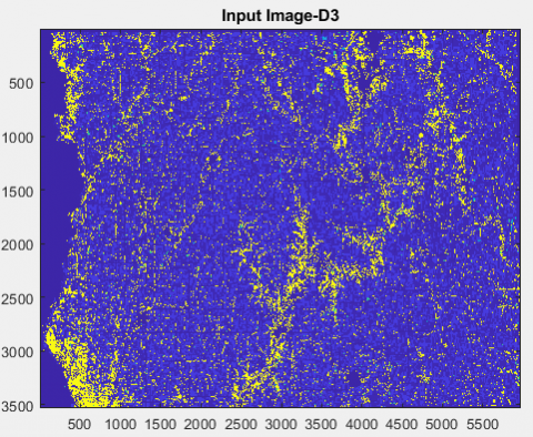
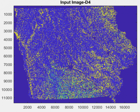
This section is the detailed illustration of the performance analysis of proposed system. The dataset of Cropland data layer is employed for estimating the algorithm’s performance. The dataset is attained by the following link (https:// nassgeodata.gmu. edu/ Crop Scape/) [21]. Table 1 is the depiction of parameter settings of proposed scheme. The Table 2 shown below illustrates the details regarding datasets. The dataset comprises of raster geo-spatial images which is being captured with resolution that are reasonable.
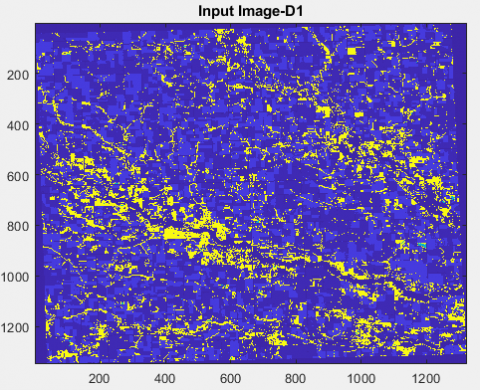
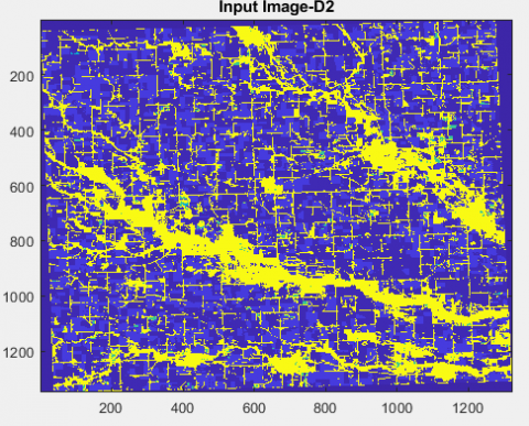
The images comprises the area of continental regions of United States, termed, Iowa state. This in turn covers over 150,000 sq.kms, at which every pixel in image covers around 900 sq meters. The various crops cultivated in the regions were identified with the use of map colors. The datasets are seperated into four datasets like D1, D2, D3, and D4 depending on the time period at which the image is required.
Table 1. Parameter settings
|
Parameter |
Parameter Description |
Value Range |
|
$\rho$ |
Neighbourhood angle for the pixels |
$0^{\circ}, 45^{\circ}, 90^{\circ}$ and $135^{\circ}$ |
|
m |
Pattern size |
8 |
|
B |
Number of binary bits |
[0,15] |
|
$L_{i}$ |
Length of the pattern matrix |
255 |
|
T |
Iteration value for decomposition |
150 |
|
‘x’ and ‘y’ |
Row and column index of the pattern |
0 to 1024 (depends upon image size) |
|
‘m’ and ‘n’ |
Number of rows and columns of the pattern |
1024 and 1024 (depends upon image size) |
|
$P_{i}$ |
Vector of unique values of pattern pixels |
4 to 8 dimension and range depend upon intensity region |
|
$E n c_{v e c}$ |
Encoded vector |
Vector of count of occurrence (50 to 100) |
Table 2. Dataset details
|
Dataset ID |
Region |
Pixel’s count |
Time duration |
Volume of data |
|
Dataset-D1 |
Smaller portion of butler country |
21* 132 |
From 2010 to 2016 |
1.7 MB |
|
Dataset-D2 |
Regions of butler country |
1323*1348 |
From 2010 to 2016 |
20 MB |
|
Dataset-D3 |
Region of ASD 1910 |
5971*3534 |
From 2010 to 2016 |
141 MB |
|
Dataset-D4 |
Region of IOWA state |
17,795*11,671 |
From 2010 to 2016 |
594 MB |
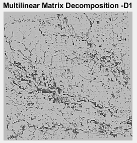
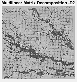
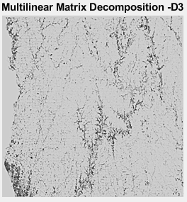
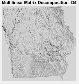
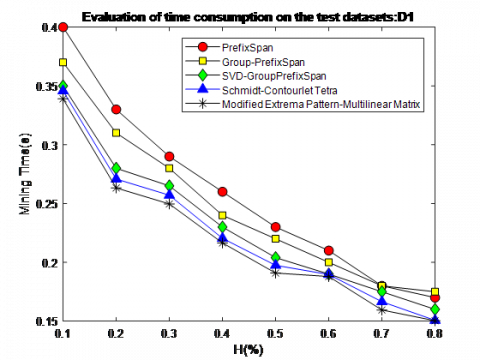
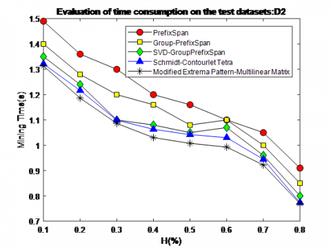
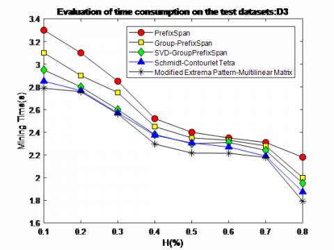
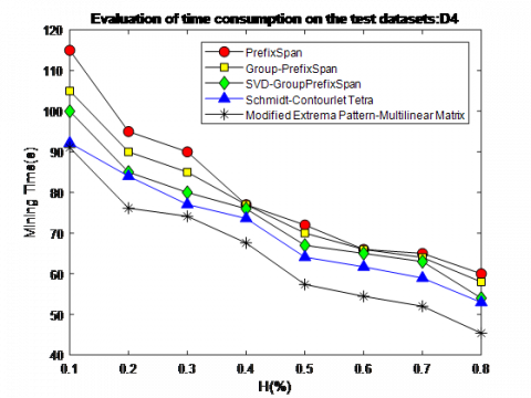
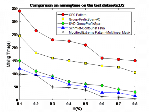
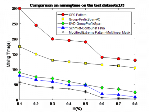
Table 3 is the comparision made with existing technqiues. The Tables 4 and 5 values are plotted as graphs in Figures 5 and 6 as a representation of graphical visualization. Figure 3 is the representation of input datasets D1, D2, D3, and D4. Similarly, Figure 4 illustrates the depiction of multilinear matrix decomposition of datasets D1, D2, D3 and D4. The analysis of time consumption on test dataset D1, D2, D3, and D4 is shown below in Figure 5 (a) (b), (c), (d). the analysis is made and the outcome is compared with existing techniques to prove the efficiency of proposed system over existing system. The analysis of mining time on test dataset D1, D2, D3, and D4 is shown below in figure 6 (a) (b), (c), (d). Table 7 is the illustration of performance analysis of compression ratio for test datasets D1, D2, D3, and D4. The compression ratio for D1 is 6.11, D2 it is 6.38, for D3 it is 6.01, and for D4 it is 5.94. Comparison of the support values of sequential pattern mining methods is given in Figure 7. Table 6 is the comparison made for the support values of the sequential pattern methods for each pattern.
4.1 Performance analysis
The proposed Modified Extrema Pattern with Multi-linear decomposition is employed proposed for enhancing the mining efficacy of spatial sequential patterns from raster serial remote sensing images (SRSI) based on pixel grouping approach. The pattern features are computed by transformation process from which the multilinear matrix decomposition of the image is made by computing the covariance estimation on recognizing their orthogonal component. The matrix decomposition is then attained based on run length encoding process (RLC). The high level of information is retained from the non-repeated pixel-based approach. From the proposed compression process, the information of structure and texture is not lost. The estimation is made and the outcome is compared with existing techniques to prove the efficiency of proposed system over existing system. The outcomes shows that the proposed system is effective to overcome the traditional issues in SRSI images.
Table 3. Comparision with existing methodologies
|
Reference |
Methodology Used |
Advantage |
Disadvantage |
|
[15] |
Spatial sequential patterns |
All patterns are extracted with a lower time cost |
IT is not capable of mining local sequential patterns with varied local thresholds |
|
[17] |
Adaptive spatial pooling (ASP) module |
It is capable of exploiting spatial context at both global and local levels |
The HRNet reduces the spatial size of the input data in its early layers to avoid intensive calculations |
|
[21] |
Spatial stratified heterogeneity |
High reliability |
This paper only focuses on the optimal choice of the scale parameter in segmentation quality evaluation. |
|
[25] |
Sparse SVM classifier, Wavelet transform |
It can optimally enhance the classification accuracy of any multispectral satellite image |
It is not applicable for change detection and environmental monitoring |
|
[28] |
Multiple classifier combination (MCC) algorithm |
Better performance in land cover classification |
Failed to encode and decode |
|
(a). Input image of Dataset D1 |
(b). Input image of Dataset D2 |
|
(c). Input image of Dataset D3 |
(d). Input image of Dataset D4 |
Figure 3. Input images of Dataset D1, D2, D3 and D4
|
(a) Multilinear matrix decomposition of Dataset 1 |
(b) Multilinear matrix decomposition of Dataset 2 |
|
(c) Multilinear matrix decomposition of Dataset 3 |
(d) Multilinear matrix decomposition of Dataset 1 |
Figure 4. Multilinear matrix decomposition of Dataset D1, D2, D3 and D4
Table 4. Mining time of prefix span, group-prefix span and modified extrema pattern-multilinear matrix based on the threshold
|
Dataset |
Threshold H(%) |
Prefix Span |
Group-Prefix Span |
SVD- Group Prefix Span |
Schmidt-Contourlet Tetra |
Modified Extrema Pattern-Multilinear Matrix |
|
Dataset D1 |
0.1 |
0.4 |
0.37 |
0.35 |
0.35 |
0.34 |
|
0.2 |
0.33 |
0.31 |
0.28 |
0.27 |
0.263 |
|
|
0.3 |
0.29 |
0.28 |
0.265 |
0.26 |
0.249 |
|
|
0.4 |
0.26 |
0.24 |
0.23 |
0.22 |
0.216 |
|
|
0.5 |
0.23 |
0.22 |
0.204 |
0.197 |
0.19 |
|
|
0.6 |
0.21 |
0.2 |
0.19 |
0.189 |
0.187 |
|
|
0.7 |
0.18 |
0.18 |
0.175 |
0.166 |
0.159 |
|
|
0.8 |
0.17 |
0.175 |
0.16 |
0.150 |
0.15 |
|
|
Dataset D2 |
0.1 |
1.49 |
1.40 |
1.35 |
1.32 |
1.31 |
|
0.2 |
1.36 |
1.28 |
1.24 |
1.21 |
1.18 |
|
|
0.3 |
1.30 |
1.20 |
1.10 |
1.09 |
1.08 |
|
|
0.4 |
1.20 |
1.16 |
1.08 |
1.063 |
1.03 |
|
|
0.5 |
1.16 |
1.08 |
1.05 |
1.04 |
1.00 |
|
|
0.6 |
1.10 |
1.10 |
1.07 |
1.03 |
0.99 |
|
|
0.7 |
1.05 |
1.00 |
0.96 |
0.94 |
0.92 |
|
|
0.8 |
0.91 |
0.85 |
0.80 |
0.77 |
0.76 |
|
|
Dataset D3 |
0.1 |
3.30 |
3.10 |
2.95 |
2.85 |
2.78 |
|
0.2 |
3.10 |
2.90 |
2.80 |
2.76 |
2.75 |
|
|
0.3 |
2.85 |
2.75 |
2.60 |
2.57 |
2.56 |
|
|
0.4 |
2.52 |
2.45 |
2.38 |
2.37 |
2.29 |
|
|
0.5 |
2.40 |
2.35 |
2.30 |
2.3 |
2.21 |
|
|
0.6 |
2.35 |
2.33 |
2.31 |
2.27 |
2.21 |
|
|
0.7 |
2.31 |
2.28 |
2.24 |
2.18 |
2.17 |
|
|
0.8 |
2.18 |
2.00 |
1.95 |
1.87 |
1.79 |
|
|
Dataset D4 |
0.1 |
115 |
105 |
100 |
92 |
91 |
|
0.2 |
95 |
90 |
85 |
84 |
76 |
|
|
0.3 |
90 |
85 |
80 |
77 |
74 |
|
|
0.4 |
77 |
77 |
76 |
74 |
68 |
|
|
0.5 |
72 |
70 |
67 |
64 |
57 |
|
|
0.6 |
66 |
66 |
65 |
62 |
54 |
|
|
0.7 |
65 |
64 |
63 |
59 |
52 |
|
|
0.8 |
60 |
58 |
54 |
53 |
45 |
|
(a) Analysis of time consumption of test dataset D1 (17.65% decreased) |
(b) Analysis of time consumption of test dataset D2 (18.11% decreased) |
|
(c) Analysis of time consumption of test dataset D3 (16.20% decreased) |
(d) Analysis of time consumption of test dataset D4 (36.90% decreased) |
Figure 5. Analysis of time consumption of test dataset D1 (17.65% decreased) b Analysis of time consumption of test dataset D2 (18.11% decreased) c Analysis of time consumption of test dataset D3 (16.20% decreased) d Analysis of time consumption of test dataset D4 (36.90% decreased)
Table 5. Mining time of GFS patten, group prefix span—AC and Modified Extrema Pattern-Multilinear Matrix based on the threshold values
|
Dataset |
Threshold H (%) |
Prefix Span |
Group-Prefix Span |
SVD- Group Prefix Span |
Schmidt-Contourlet Tetra |
Modified Extrema Pattern-Multilinear Matrix |
|
Dataset D1 |
0.1 |
360 |
260 |
180 |
144 |
96 |
|
0.2 |
290 |
190 |
100 |
66 |
49 |
|
|
0.3 |
250 |
180 |
80 |
62 |
39 |
|
|
0.4 |
245 |
170 |
85 |
51 |
33 |
|
|
0.5 |
240 |
140 |
60 |
46 |
21 |
|
|
0.6 |
220 |
138 |
55 |
34 |
9 |
|
|
0.7 |
210 |
130 |
40 |
27 |
5 |
|
|
0.8 |
205 |
125 |
30 |
5 |
3 |
|
|
Dataset D2 |
0.1 |
340 |
245 |
150 |
141 |
98 |
|
0.2 |
265 |
180 |
110 |
90 |
94 |
|
|
0.3 |
230 |
160 |
90 |
56 |
49 |
|
|
0.4 |
225 |
150 |
70 |
48 |
46 |
|
|
0.5 |
210 |
140 |
60 |
35 |
38 |
|
|
0.6 |
160 |
130 |
55 |
30 |
12 |
|
|
0.7 |
155 |
125 |
40 |
13 |
10 |
|
|
0.8 |
150 |
105 |
30 |
9 |
4 |
|
|
Dataset D3 |
0.1 |
300 |
175 |
90 |
80 |
57 |
|
0.2 |
245 |
150 |
75 |
66 |
44 |
|
|
0.3 |
200 |
130 |
70 |
60 |
40 |
|
|
0.4 |
195 |
125 |
60 |
48 |
36 |
|
|
0.5 |
190 |
120 |
50 |
47 |
26 |
|
|
0.6 |
140 |
115 |
40 |
20 |
7 |
|
|
0.7 |
135 |
112 |
35 |
17 |
5 |
|
|
0.8 |
130 |
105 |
25 |
9 |
3 |
|
|
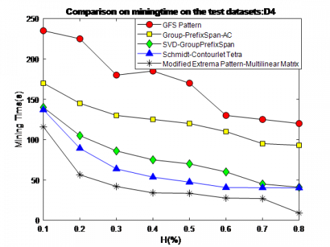
Dataset D4 |
0.1 |
235 |
170 |
140 |
137 |
115 |
|
0.2 |
225 |
145 |
105 |
89 |
56 |
|
|
0.3 |
180 |
130 |
86 |
64 |
42 |
|
|
0.4 |
185 |
125 |
75 |
53 |
34 |
|
|
0.5 |
170 |
120 |
70 |
47 |
33 |
|
|
0.6 |
130 |
110 |
60 |
41 |
28 |
|
|
0.7 |
125 |
95 |
45 |
40 |
27 |
|
|
0.8 |
120 |
93 |
41 |
40 |
9 |
|
(a) Analysis of mining time of test dataset D1 (57.75% decreased) |
(b) Analysis of mining time of test dataset D1 (72.46% decreased) |
|
(c) Analysis of mining time of test dataset D3 (83.33% decreased) |
(d) Analysis of mining time of test dataset D4 (68.75% decreased) |
Figure 6. Analysis of mining time of test dataset D1 (57.75% decreased) b Analysis of mining time of test dataset D1 (72.46% decreased) c Analysis of mining time of test dataset D3 (83.33% decreased) d Analysis of mining time of test dataset D4 (68.75% decreased)
Table 6. Support values of sequential pattern methods for each pattern
|
Pattern |
Support of patterns produced by Prefix Span |
Support of patterns produced by Prefix Span Group- Prefix Span |
Support of patterns produced by Prefix Span SVD- Group Prefix Span |
Support of patterns produced by Schmidt-Contourlet Tetra |
Support of patterns produced by Modified Extrema Pattern-Multilinear Matrix |
|
P1 |
1280000 |
1000000 |
950000 |
943190 |
937697 |
|
P2 |
1200000 |
1020000 |
980000 |
974863 |
969153 |
|
P3 |
1180000 |
1030000 |
985000 |
977107 |
971266 |
|
P4 |
900000 |
900000 |
890000 |
883116 |
877135 |
|
P5 |
1050000 |
900000 |
850000 |
843609 |
837022 |
|
P6 |
950000 |
950000 |
900000 |
890308 |
883726 |
|
P7 |
1100000 |
900000 |
880000 |
870219 |
864131 |
|
P8 |
1050000 |
1050000 |
1000000 |
992957 |
986702 |
|
P9 |
910000 |
890000 |
850000 |
842109 |
832644 |
|
P10 |
1150000 |
890000 |
800000 |
791383 |
782867 |
|
P11 |
1100000 |
1000000 |
900000 |
894786 |
887007 |
|
P12 |
1000000 |
950000 |
850000 |
842241 |
836319 |
|
P13 |
950000 |
920000 |
880000 |
872106 |
866046 |
|
P14 |
980000 |
908760 |
900000 |
894918 |
889532 |
|
P15 |
905000 |
900000 |
895000 |
887608 |
878039 |
Figure 7. Comparison of the support values of sequential pattern mining methods
Table 7. Compression ratio analysis for test datasets
|
Dataset |
D1 |
D2 |
D3 |
D4 |
|
Compression ratio |
6.11 |
6.38 |
6.01 |
5.94 |
A spatial sequential pattern mining from the high-resolution and huge volume remote sensing image sets is considered as a huge challenging aspect. The new technique of modified extrema pattern and multilinear matrix decomposition-based run length encoding process is presented for spatial sequential pattern mining. The presented approach is highly competent since it is capable of compressing the sets of remote sensing images by means of pixel grouping scheme. The algorithms employed were estimated and are validated with the use of cropland data layer datasets and the outcomes attained were compared with existing techniques to prove the efficiency of proposed system in terms of mining time and time consumption which in turn generates suitable sequence patterns beyond the support values. thus, the presented approach is said to be effective as it compresses SRSI effectively.
[1] Jia, X., Li, S., Khandelwal, A., Nayak, G., Karpatne, A., Kumar, V. (2019). Spatial context-aware networks for mining temporal discriminative period in land cover detection. Proceedings of the 2019 SIAM International Conference on Data Mining, pp. 513-521. https://doi.org/10.1137/1.9781611975673.58
[2] Mishra, V.N., Kumar, V., Prasad, R., Punia, M. (2021). Geographically weighted method integrated with logistic regression for analyzing spatially varying accuracy measures of remote sensing image classification. Journal of the Indian Society of Remote Sensing, 49: 1189-1199. https://doi.org/10.1007/s12524-020-01286-2
[3] You, H., Tian, S., Yu, L., Lv, Y. (2019). Pixel-level remote sensing image recognition based on bidirectional word vectors. IEEE Transactions on Geoscience and Remote Sensing, 58(2): 1281-1293. https://doi.org/10.1109/TGRS.2019.2945591
[4] Xue, Y., Li, T., Liu, Z., Pang, C., Li, M., Liao, Z., Hu, X. (2018). A new approach for the deep order preserving submatrix problem based on sequential pattern mining. International Journal of Machine Learning and Cybernetics, 9: 263-279. https://doi.org/10.1007/s13042-015-0384-z
[5] Zhang, L., Liu, Z., Ren, T., Liu, D., Ma, Z., Tong, L., Zhang, C., Zhou, T., Zhang, X., Li, S. (2020). Identification of seed maize fields with high spatial resolution and multiple spectral remote sensing using random forest classifier. Remote Sensing, 12(3): 362. https://doi.org/10.3390/rs12030362
[6] Wu, C., Li, X., Chen, W., Li, X. (2020). A review of geological applications of high-spatial-resolution remote sensing data. Journal of Circuits, Systems and Computers, 29(6): 2030006. https://doi.org/10.1142/S0218126620300068
[7] Wylie, B.K., Pastick, N.J., Picotte, J.J., Deering, C.A. (2019). Geospatial data mining for digital raster mapping. GIScience & Remote Sensing, 56(3): 406-429. https://doi.org/10.1080/15481603.2018.1517445
[8] Gan, W., Lin, J.C.W., Fournier-Viger, P., Chao, H.C., Yu, P.S. (2019). A survey of parallel sequential pattern mining. ACM Transactions on Knowledge Discovery from Data (TKDD), 13(3): 1-34. https://doi.org/10.1145/3314107
[9] Zhang, C., Wei, S., Ji, S., Lu, M. (2019). Detecting large-scale urban land cover changes from very high resolution remote sensing images using CNN-based classification. ISPRS International Journal of Geo-Information, 8(4): 189. https://doi.org/10.3390/ijgi8040189
[10] Xu, X., Chen, Y., Zhang, J., Chen, Y., Anandhan, P., Manickam, A. (2021). A novel approach for scene classification from remote sensing images using deep learning methods. European Journal of Remote Sensing, 54(2): 383-395. https://doi.org/10.1080/22797254.2020.1790995
[11] He, Z., Zhang, S., Wu, J. (2019). Significance-based discriminative sequential pattern mining. Expert Systems with Applications, 122: 54-64. https://doi.org/10.1016/j.eswa.2018.12.046
[12] Cai, G., Lee, ., Lee, I. (2018). Itinerary recommender system with semantic trajectory pattern mining from geo-tagged photos. Expert Systems with Applications, 94: 32-40. https://doi.org/10.1016/j.eswa.2017.10.049
[13] Tiwari, P., Shukla, P.K. (2019). A review on various features and techniques of crop yield prediction using geo-spatial data. International Journal of Organizational and Collective Intelligence (IJOCI), 9(1): 37-50. https://doi.org/10.4018/IJOCI.2019010103
[14] Wei, J., Mi, L., Hu, Y., Ling, J., Li, Y., Chen, Z. (2022). Effects of lossy compression on remote sensing image classification based on convolutional sparse coding. IEEE Geoscience and Remote Sensing Letters, 19: 1-5. https://doi.org/10.1109/LGRS.2020.3047789
[15] Wu, X., Zhang, X. (2019). An efficient pixel clustering-based method for mining spatial sequential patterns from serial remote sensing images. Computers & Geosciences, 124: 128-139. https://doi.org/10.1016/j.cageo.2019.01.005
[16] Jing, W., Huo, S., Miao, Q., Chen, X. (2017). A model of parallel mosaicking for massive remote sensing images based on spark. IEEE Access, 5: 18229-18237. https://doi.org/10.1109/ACCESS.2017.2746098
[17] Zhang, J., Lin, S., Ding, L., Bruzzone, L. (2020). Multi-scale context aggregation for semantic segmentation of remote sensing images. Remote Sensing, 12(4): 701. https://doi.org/10.3390/rs12040701
[18] Ding, L., Tang, H., Bruzzone, L. (2020). LANet: Local attention embedding to improve the semantic segmentation of remote sensing images. IEEE Transactions on Geoscience and Remote Sensing, 59(1): 426-435. https://doi.org/10.1109/TGRS.2020.2994150
[19] Song, J., Zhang, H., Li, X., Gao, L., Wang, M., Hong, R. (2018). Self-supervised video hashing with hierarchical binary auto-encoder. IEEE Transactions on Image Processing, 27(7): 3210-3221. https://doi.org/10.1109/TIP.2018.2814344
[20] Song, J., Guo, Y., Gao, L., Li, X., Hanjalic, A., Shen, H.T. (2018). From deterministic to generative: Multimodal stochastic RNNs for video captioning. IEEE Transactions on Neural Networks and Learning Systems, 30(10): 3047-3058. https://doi.org/10.1109/TNNLS.2018.2851077
[21] Gao, H., Tang, Y., Jing, L., Li, H., Ding, H. (2017). A novel unsupervised segmentation quality evaluation method for remote sensing images. Sensors, 17(10): 2427. https://doi.org/10.3390/s17102427
[22] Zhang, Z., He, Q., Tong, H., Gou, J., Li, X. (2016). Spatial-temporal traffic flow pattern identification and anomaly detection with dictionary-based compression theory in a large-scale urban network. Transportation Research Part C: Emerging Technologies, 71: 284-302. https://doi.org/10.1016/j.trc.2016.08.006
[23] Das, P., Pandey, V. (2019). Use of logistic regression in land-cover classification with moderate-resolution multispectral data. Journal of the Indian Society of Remote Sensing, 47: 1443-1454. https://doi.org/10.1007/s12524-019-00986-8
[24] Al-Ahmadi, F., Hames, A. (2009). Comparison of four classification methods to extract land use and land cover from raw satellite images for some remote arid areas, Kingdom of Saudi Arabia. Earth, 20(1): 167-191.
[25] Menaka, D., Padmasuresh, L., Selvin Prem Kumar, S. (2015). Classification of multispectral satellite images using sparse SVM classifier. Indian J Sci Technol, 8: 1-7.
[26] Lyu, X., Ma, H. (2019). An efficient incremental mining algorithm for discovering sequential pattern in wireless sensor network environments. Sensors, 19(1): 29. https://doi.org/10.3390/s19010029
[27] Dong, X., Zheng, Z., Cao, L., Zhao, Y., Zhang, C., Li, J., Wei, W., Ou, Y. (2011). e-NSP: Efficient negative sequential pattern mining based on identified positive patterns without database rescanning. Proceedings of the 20th ACM International Conference on Information and Knowledge Management, pp. 825-830. https://doi.org/10.1145/2063576.2063695
[28] Shen, H., Lin, Y., Tian, Q., Xu, K., Jiao, J. (2018). A comparison of multiple classifier combinations using different voting-weights for remote sensing image classification. International Journal of Remote Sensing, 39(11): 3705-3722. https://doi.org/10.1080/01431161.2018.1446566
[29] Ye, D., Li, Y., Tao, C., Xie, X., Wang, X. (2017). Multiple feature hashing learning for large-scale remote sensing image retrieval. ISPRS International Journal of Geo-Information, 6(11): 364. https://doi.org/10.3390/ijgi6110364
[30] Häberle, M., Werner, M., Zhu, X.X. (2019). Geo-spatial text-mining from Twitter–a feature space analysis with a view toward building classification in urban regions. European Journal of Remote Sensing, 52: 2-11. https://doi.org/10.1080/22797254.2019.1586451
[31] Zhang, X., Liu, R., Gan, F., Wang, W., Ding, L., Yan, B. (2020). Evaluation of spatial-temporal variation of vegetation restoration in dexing copper mine area using remote sensing data. IGARSS 2020-2020 IEEE International Geoscience and Remote Sensing Symposium, pp. 2013-2016. https://doi.org/10.1109/IGARSS39084.2020.9323698
[32] Preethi, R.A., Anandharaj, G. (2020). Quantized ternary pattern and singular value decomposition for the efficient mining of sequences in SRSI images. SN Applied Sciences, 2: 1-14. https://doi.org/10.1007/s42452-020-03474-8