Aloui Noureddine* | Mohamed Boussif | Cherif Adnane
© 2022 IIETA. This article is published by IIETA and is licensed under the CC BY 4.0 license (http://creativecommons.org/licenses/by/4.0/).
OPEN ACCESS
In this paper an improved ultraspherical window is developed for designing quadrature mirror filters banks (QMF) with the help of a real coded genetic algorithm (RCGA). In fact, the ultraspherical window is modified by adding a parameter (α) which to improve the spectral parameters. Then, RCGA is used to find optimal values of the adjustment parameters, the side-lobes ratio of ultraspherical window and the cut-off frequency of the low-pass prototype filter. This latter, is used to derive all the filters of QMF banks. When the developed QMF banks are exploited for speech enhancement algorithm based on wavelets techniques it gives good performances in terms of Perceptual Evaluation of Speech Quality (PESQ) and Signal to Noise Ratio (SNR). In addition to this, when compared to Dolph-Chebyshev, Kaiser and the original Ultraspherical windows the modified Ultraspherical window gives better performance referred to the obtained simulation results.
ultraspherical window, quadrature mirror filters banks, speech enhancement, discrete wavelet transforms
In digital signal processing (DSP) the analysis window is a mathematical function that is zero valued outside of a given interval. It is widely used in many applications of DSP such as spectral analysis [1], digital filters design [2], beam forming techniques [3] and antenna design [4]. The window function can be classified into two types. The first type is known as fixed window function it has only one single parameter called window length, which is used to control the main lobe width. The Hanning, Hamming, Blackman, Triangular and Rectangular window are some examples of fixed window functions [5]. The second type, known as adjustable window function, it has one or more adjustment parameters besides the window length, which are used to improve spectral characteristics, among them is Kaiser [6], Dolph-Chebyshev [7], Cosh [8], ultraspherical [9] and Saramaki [10] windows. In fact, the Kaiser window approximates the discrete prolate spheroidal sequence function (DPSS), which have the particularity of maximum energy concentration in the main lobe. The Dolph-Chebyshev window is controlled by two parameters to produce minimum main lobe width for a specified maximum side-lobe. The ultraspherical window has three parameters that control the side lobes amplitude relative to the main lobe.
During the last decades a lot of effort has been made to design and optimize analysis window functions with desired specifications for different applications of signal processing. In fact, Kumar and Kuldeep [11] present an improved Dolph-Chebyshev window function by adding a third parameter (α) to improve the spectral characteristics in terms of smaller ripple ratio and the wider main lobe width. Then the developed window was exploited for designing QMF banks, and it gives better performance in term of computational time, amplitude distortion and aliasing distortion compared to others modified Kaiser and Cosh window. A new window function is developed using the product of Hamming and Gaussian windows [12], it offers better spectral parameters in term of minimum side lobe peak. When it is exploited for FIR filters design it achieves minimum ripple ratio compared to the designed filters using the Hamming, Blackman, Gaussian, and Kaiser windows. Therefore, in this paper modified ultraspherical window function is developed and used for designing QMF banks. This latter, are exploited to enhance speech signals. The paper is organized as follows. Section 2 explains the principle of analysis and synthesis using QMF banks. Section 3, presents the optimized ultraspherical window. Section 4, discusses the QMF banks design using modified ultraspherical window and RCGA. The methodology of speech enhancement based on wavelet techniques is given in section 5. Section 6, depicts simulation results and comparative study of performances. Finally, a conclusion is given in section 7.
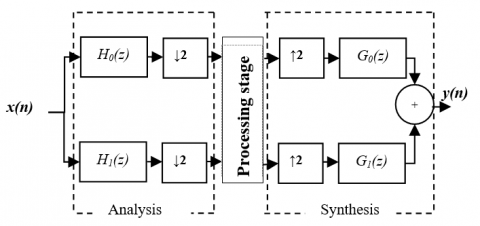
QMF is a two channel filter bank, which the principle consists of decomposing an input signal x(n) into two sub-bands using a low-pass analysis filter H0(z) and a high-pass analysis filter H1(z). The obtained sub-bands are down-sampled by a factor of 2. After a processing stage, each sub-band is up-sampled by a factor of 2 and passing through a low-pass synthesis filter G0(z) and high-pass synthesis filter G1(z). Finally, to reconstruct the output signal y(n) the sub-bands are recombined. Figure 1 shows the block diagram of QMF [13-17].
Figure 1. A general structure of two channels QMF bank
The relationship between the x(n) and y(n) signals in z-transform is expressed as:
$Y(z)=\frac{1}{2}\left[H_{0}(z) G_{0}(z)+H_{1}(z) G_{1}(z)\right] X(z)$
$+\frac{1}{2}\left[H_{0}(-z) G_{0}(z)+H_{1}(-z) G_{1}(z)\right] X(-z)$ (1)
For QMF banks design there are three types of distortion can be occurred; aliasing, phase and amplitude distortions. The aliasing distortion is due to the non-idealness of the designed filters, which can be eliminated by the use of a suitable design of the synthesis filters: G0(z)=H1(-z) and G1(z)=-H0(-z). The phase distortion is caused by the nonlinear phase response of the filter; it can be eliminated by the use of a linear phase FIR $\left(\left|H_{0}\left(e^{j \omega}\right)\right| e^{-j \omega(N-1) / 2}\right)$ of even length (N). The amplitude distortion (or peak reconstruction error (PRE)), can never be eliminated completely. Then, the Eq. (1) becomes:
$Y(z)=\frac{1}{2}\left[H_{0}^{2}(z)+\mathrm{H}_{0}^{2}(-\mathrm{z})\right] X(z)$ (2)
Let $F(z)=\frac{Y(z)}{X(z)}$ , the Eq. (2) becomes:
$F(z)=\frac{1}{2}\left[H_{0}^{2}(z)+\mathrm{H}_{0}^{2}(-\mathrm{z})\right]$ (3)
Then, the frequency response of the QMF filter bank can be expressed as follows:
$\begin{aligned} F\left(e^{j \omega}\right)=& \frac{Y\left(e^{j \omega}\right)}{X\left(e^{j \omega}\right)}=\frac{e^{-j \omega(N-1)}}{2}\left[\left|H_{0}\left(e^{j \omega}\right)\right|^{2}-\right.\\ &\left.(-1)^{N-1}\left|H_{0}\left(e^{j(\omega-\pi)}\right)\right|^{2}\right] \end{aligned}$ (4)
where, $z=e^{j \omega}$ and $H_{0}\left(e^{j \omega}\right)=\left|H_{0}\left(e^{j \omega}\right)\right| e^{-j \omega(N-1) / 2}$ .
The condition of perfect reconstruction implies that the QMF bank has a magnitude response $F\left(e^{j \omega}\right)$ must be unity:
$F\left(e^{j \omega}\right)=\left(\left|H_{0}\left(e^{j \omega}\right)\right|^{2}+\left|H_{0}\left(e^{j(\omega-\pi)}\right)\right|^{2}=1\right.$ (5)
If this equation is evaluated at frequency (ω=0.5π), the perfect reconstruction condition reduces as follow: $\left|H_{0}\left(e^{j \frac{\omega}{2}}\right)\right|$ =0.707.
If this condition is not satisfied then a PRE is occurred, which can be expressed using the following equation [18]:
$P R E=\max \left\{20 \log \left(\left|H_{0}\left(e^{j \omega}\right)\right|^{2}+\right.\right.$
$\left.\left.\left|H_{0}\left(e^{j(\omega-\pi)}\right)\right|^{2}\right)\right\}$ (6)
It can be remark from the above equation that the PRE function can be minimized by the use of appropriate prototype filter. Thus, for filter design using windowing techniques the choice of window function carefully allows for maximizing the prototype filter quality.
The ultraspherical window of length N can be expressed as [19]:
$W(n)=\frac{1}{N+1}\left[C_{N}^{\mu}\left(x_{0}\right)+\right.$
$\left.\sum_{k=1}^{\frac{N}{2}} C_{N}^{\mu}\left(x_{0} \cos \left(\frac{k \pi}{N+1}\right)\right) \cos \left(\frac{2 n k \pi}{N+1}\right)\right]$ (7)
where, $C_{N}^{\mu}(x)$ represents the ultraspherical polynomial or Gegenbauer polynomials, it can be expressed as follow:
$C_{N}^{\mu}(x)=\frac{1}{N}\left[2(N+\mu-1) x C_{N-1}^{\mu}(x)+(N+2 \mu-\right.$ $\left.2) C_{N-2}^{\mu}(x)\right]$ (8)
$C_{1}^{\mu}=2 \mu x$ (9)
$C_{2}^{\mu}=-\mu+2 \mu(1+\mu) x^{2}$ (10)
The parameter μ controls the window Fourier transform side-lobe roll-off ratio and the parameter x0 provides a trade-off between the ripple-ratio and a width characteristic. For μ→0 the Eq. (11) gives Dolph-Chebyshev window function, μ≈3-4 gives Hann window and for 0<μ<-1 the side lobes increase in magnitude with frequency.
For filter design using ultraspherical window these parameters must be chosen such that the filter specifications are satisfied [20].
In this work, the original ultraspherical window is modified by adding a parameter (α) which to improve the spectral characteristics in terms of the ripple ratio and side-lobe roll-off ratio. The modified ultraspherical window can be expressed as follow:
$\omega(n)=\frac{1}{(N+1)^{\alpha}}\left[C_{N}^{\mu}\left(x_{0}\right)+\right.$
$\left.\sum_{k=1}^{\frac{N}{2}} C_{N}^{\mu}\left(x_{0} \cos \left(\frac{k \pi}{N+1}\right)\right) \cos \left(\frac{2 n k \pi}{N+1}\right)\right]^{\alpha}$ (11)
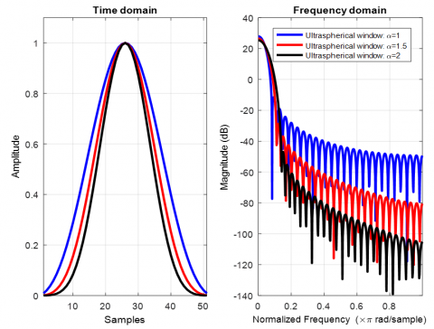
Figure 2 and the corresponding data given at Table 1 shows the effect of the adjustable parameter (α) on the ultraspherical window spectrum for constants values of μ=2 at x0=1.005 and window length N=51:
It is clear from Figure 2 and Table 1 that the increments of the adjustment parameter (α) implies an increase of the main lobe width decrease the ripple ratio and the side-lobe roll-off ratio for fixed values of μ=2 and x0= 1.005. Therefore, the adjustment parameter makes the modified ultraspherical window more flexible compared to the classical ultraspherical window.
Figure 2. Effect of the adjustment parameter (α) on the ultraspherical window
Table 1. Comparison of the spectral parameters for different values of adjustment parameter (α)
|
Window |
α |
ωR(rad/s) |
Ripple ratio (dB) |
Side-lobe roll-off ratio |
|
Ultraspherical window |
1 |
0.083 |
37.788 |
27.104 |
|
Modified ultraspherical window |
1.5 |
0.111 |
55.173 |
51.485 |
|
Modified ultraspherical window |
2 |
0.142 |
72.152 |
58.011 |
In this section, real coded genetic algorithm (RCGA) is exploited for finding the optimal spectral parameters (μ, x0, α) of modified ultraspherical window and the cutoff frequency (ωc) of the prototype filter, in order to develop efficient QMF banks.
Generally, genetic algorithms (GA) are optimization techniques inspired by natural evolution. They are used to generate efficient solutions to optimization problems by relying on biologically inspired operators such as: selection, crossover and mutation.
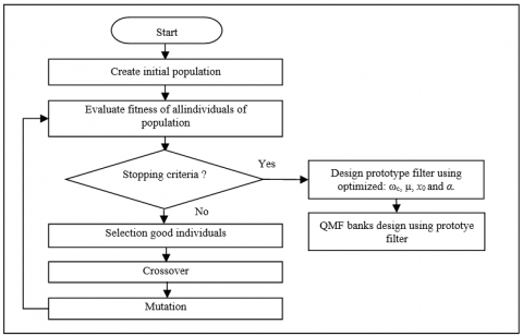
Figure 3 illustrates the flowchart of the RCGA used for optimizing the prototype filter parameters, which it is involves a number of different steps adapted for designing prototype filters.
Step 1. create a random initial population of chromosomes:
Figure 3. A flowchart of QMF banks design using GA
initial population =$\left(\begin{array}{cccc}{\left[\omega_{c 1}\right.} & \mu_{1} & x_{01} & \left.\alpha_{1}\right]_{1} \\ {\left[\omega_{c 2}\right.} & \mu_{2} & x_{02} & \left.\alpha_{2}\right]_{2} \\ \vdots & & \vdots & \\ {\left[\omega_{c n}\right.} & \mu_{n} & x_{0 n} & \left.\alpha_{n}\right]_{n}\end{array}\right)_{0}$
where, $\omega_{c i / i=1,2, \ldots, n}$ represent the initial cutoff frequency values of the prototype filter and $\mu_{i / i=1,2, \ldots, n}, \chi_{0 i / i=1,2, \ldots, n}, \alpha_{i / i=1,2, \ldots, n}$ the initial parameters of the modified ultraspherical window function (usually μ≥1 and x0≥1).
Step 2. Evaluate the fitness functions $f\left(\omega_{c i}, \mu_{i}, x_{0 i}, \alpha_{i}\right)_{/ i=1,2, \ldots, n}$ for each individual and design the prototype filters based on modified ultraspherical window, then calculate the magnitude responses (MRC):
$M R C_{i / i=1,2, \ldots, n}=\left|e^{j \omega_{c i}}\right|$ at $\omega=\frac{\pi}{2}$ (12)
$E r_{i / i=1,2, \ldots, n}=\left|M R I-M R C_{i}\right|$ (13)
where, the magnitude response in the ideal condition (MRI) is equal to 0.707and $E r_{i / i=1,2, \ldots, n}$ is the fitness function.
Step 3. If the maximum number of generations is reached or Er≤Tol (Tol: tolerance) then RCGA algorithm stop. Otherwise RCGA algorithm repeats the following steps:
new population= $\left(\begin{array}{cccc}{\left[\omega_{c 1} \mu_{1}\right.} & x_{01} & \left.\alpha_{1}\right]_{1} \\ {\left[\omega_{c 2} \mu_{2}\right.} & x_{02} & \left.\alpha_{2}\right]_{2} \\ \vdots & \vdots & & \\ {\left[\omega_{c n} \mu_{n}\right.} & x_{0 n} & \left.\alpha_{n}\right]_{n}\end{array}\right)$
Step 4. Stop and design prototype filter using the optimized parameters.
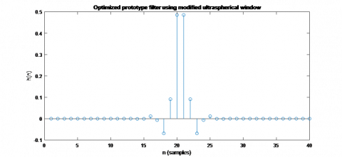
Table 2 illustrates tow optimized prototype filters using modified ultraspherical window and RCGA for different filters length (40 and50). The optimal settings of the RCGA as shown in Table 3 and the associated QMF banks are given in Figures 4 and 5.
Table 2. Optimized prototype filters coefficients based on modified ultraspherical window
|
N |
Modified Ultraspherical window: μ=2, x0= 3.552115681083168 α=1.880512388091985 $\omega_{c}$ =0.552 |
Modified Ultraspherical window: μ=2, x0=1.004381233990749, α=0.118292522778291 $\omega_{c}$ =0.5068 |
|
1 |
0.000000000000000 |
0.007405125497528 |
|
2 |
0.000000000000000 |
-0.002474905928106 |
|
3 |
-0.000000000000000 |
-0.009420210751112 |
|
4 |
-0.000000000000002 |
0.003481007245895 |
|
5 |
0.000000000000368 |
0.011163206985787 |
|
6 |
0.000000000000174 |
-0.004658644988645 |
|
7 |
-0.000000000344006 |
-0.012981123313748 |
|
8 |
0.000000001940887 |
0.006094563579390 |
|
9 |
0.000000074985647 |
0.015015805527867 |
|
10 |
-0.000000520182139 |
-0.007890395696965 |
|
11 |
-0.000004877296413 |
-0.017411232939896 |
|
12 |
0.000037401671299 |
0.010199912946942 |
|
13 |
0.000101446934606 |
0.020374492408386 |
|
14 |
-0.000991139297799 |
-0.013280669464605 |
|
15 |
-0.000420480334635 |
-0.024255874093758 |
|
16 |
0.011441470521815 |
0.017605631804231 |
|
17 |
-0.006493081366513 |
0.029726729536558 |
|
18 |
-0.068797041014316 |
-0.024151593722993 |
|
19 |
0.091129091166720 |
-0.038278959810925 |
|
20 |
0.485385977803475 |
0.035315986642234 |
|
21 |
0.485385977803475 |
0.054052516444313 |
|
22 |
0.091129091166720 |
-0.058976459541863 |
|
23 |
-0.068797041014316 |
-0.094431588343764 |
|
24 |
-0.006493081366513 |
0.145026402089081 |
|
25 |
0.011441470521815 |
0.454940713139490 |
|
26 |
-0.000420480334635 |
0.454940713139490 |
|
27 |
-0.000991139297799 |
0.145026402089081 |
|
28 |
0.000101446934606 |
-0.094431588343764 |
|
29 |
0.000037401671299 |
-0.058976459541863 |
|
30 |
-0.000004877296413 |
0.054052516444313 |
|
31 |
-0.000000520182139 |
0.035315986642234 |
|
32 |
0.000000074985647 |
-0.038278959810925 |
|
33 |
0.000000001940887 |
-0.024151593722993 |
|
34 |
-0.000000000344006 |
0.029726729536558 |
|
35 |
0.000000000000174 |
0.017605631804231 |
|
36 |
0.000000000000368 |
-0.024255874093758 |
|
37 |
-0.000000000000002 |
-0.013280669464605 |
|
38 |
-0.000000000000000 |
0.020374492408386 |
|
39 |
0.000000000000000 |
0.010199912946942 |
|
40 |
0.000000000000000 |
-0.017411232939896 |
|
41 |
|
-0.007890395696965 |
|
42 |
|
0.015015805527867 |
|
43 |
|
0.006094563579390 |
|
44 |
|
-0.012981123313748 |
|
45 |
|
-0.004658644988645 |
|
46 |
|
0.011163206985787 |
|
47 |
|
0.003481007245895 |
|
48 |
|
-0.009420210751112 |
|
49 |
|
-0.002474905928106 |
|
50 |
|
0.007405125497528 |
Table 3. Optimal RCGA parameters used for QMF banks design
|
Parameters |
Values |
|
Coding |
Real |
|
Population size |
40 |
|
Maximum number of generations |
30 |
|
Size of chromosome |
2 |
|
Cutoff $\left(\boldsymbol{\omega}_{\mathbf{c}}\right)$ |
0.49 - 0.57 |
|
μ |
1 - 6 |
|
x0 |
0-10 |
|
α |
0-2 |
|
Tolerance (tol) |
10-5 |
|
Fitness Function |
fitness =Minimize (|err-tol|) |
|
Selection Technique |
Elitist selection. |
|
Probability of selection |
0.5 |
|
Method of mutation |
Random. |
|
Mutation probability |
pmut = 0.1 |
|
Method of crossing |
One point crossover |
|
Probability of crossover |
pcross =0.5 |
|
Stopping criterion |
Maximum number of generations or fitness ≤tol |
Figure 4. Optimized prototype filter using modified ultraspherical window and RCGA (N=40)
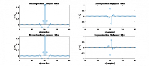
Figure 5. The associated QMF bank using modified ultraspherical window and RCGA (N=40)
In this work, the designed QMF banks using modified ultraspherical window and RCGA are exploited for speech enhancement based on discrete wavelet transform (DWT). In fact, the optimized analysis filters of two-channel QMF bank are used to decompose the noisy speech signals into sub-bands frequency. Then, the synthesis filters of two-channel QMF bank are applied to reconstruct the enhanced speech signals.
Generally, for speech enhancement based on DWT three steps most commonly used; decomposition using DWT, thresholding and reconstruction by applying inverse DWT [21-25]:
Step 1: consists in choosing the wavelet function, the decomposition level and compute the DWT in order to obtain approximation and detail coefficients of the noisy signal.
Step 2: in this step, the obtained wavelet coefficients (w(n)) are thresholded using hard thresholding or soft thresholding using the following formula:
Hard thresholding (wh(n)):
$w_{h}(n)=\left\{\begin{array}{l}w(n),|w(n)| \geq T \\ 0 \text { otherwise }\end{array}\right.$ (14)
Soft thresholding (ws(n)):
$w_{s}(n)=\left\{\begin{array}{l}\operatorname{sign}(w(n))(|w(n)|-T), w(n)>T \\ 0|w(n)| \leq T\end{array}\right.$ (15)
where, T represents the threshold value, which can be computed using many methods such as; level dependent threshold computation, global threshold computation or universal threshold computation. This latter, is most widely used due to its effectiveness and simpleness, which can be expressed as:
$T_{U}=\delta \sqrt{2 \ln (N)}$ (16)
where, σ and N are respectively the average variance of the noise and the signal length. σ can be calculated using the following formula:
$\delta=\frac{\operatorname{median}\left(\left|w_{1, i}\right|\right)}{0.6745}$ (17)
$w_{1, i}$ represents all wavelet coefficients at scale one.
Step 3: in this steps IDWT is applied to reconstruct enhanced signal using original approximation coefficients and modified detail coefficients.
For the evaluation a MATLAB program has been written to implement the speech enhancement algorithm based on wavelets techniques, which exploit the optimized QMF banks based on modified ultraspherical window and RCGA.
A speech dataset token from the study [15] was used to evaluate the effectiveness of the optimized QMF banks. The noise signals were added to the speech signals at SNRs of 5dB and 10dB. The comparative study of performance was performed in terms of Perceptual Evaluation of Speech Quality (PESQ) and the Signal to Noise Ratio (SNR).
Tables 4, 5 and Figure 6 show the simulation results of SNR (dB) and PESQ score obtained using different window functions for QMF banks design. For speech enhancement algorithm using wavelet techniques, each selected test signal (“Babble.wav” and “Train.wav”) is decomposed by using optimized QMF banks into 5 levels, soft thresholding is applied to the obtained coefficients using universal threshold value and a single estimation of noise level based on first level of wavelet coefficients.
Table 4. Comparison performances of the designed QMF banks for “Babble” test signal
|
Window |
N |
ωc |
SNR=5dB |
SNR=10dB |
||
|
SNR(dB) |
PESQ |
SNR(dB) |
PESQ |
|||
|
Dolph-Chebyshev: As=60 |
40 |
0.5 |
4.786 |
1.817 |
8.849 |
2.072 |
|
Kaiser: β=8 |
40 |
0.5 |
4.806 |
1.816 |
8.726 |
2.068 |
|
Ultraspherical: μ=2, x0=3 |
40 |
0.5 |
5.126 |
1.761 |
7.355 |
2.028 |
|
Modified ultraspherical: μ=2, x0=3.552115681083168 α=1.880512388091985 |
40 |
0.552 |
5.556 |
1.882 |
9.661 |
2.095 |
Table 5. Comparison performances of the designed QMF banks for “Train” test signal
|
Window |
N |
ωc |
SNR=5dB |
SNR=10dB |
||
|
SNR(dB) |
PESQ |
SNR(dB) |
PESQ |
|||
|
Dolph-Chebyshev: As=60 |
50 |
0.5 |
6.901 |
0.850 |
9.841 |
1.409 |
|
Kaiser: β=8 |
50 |
0.5 |
6.864 |
0.841 |
9.680 |
1.418 |
|
Ultraspherical: μ=2, x0=1 |
50 |
0.5 |
6.974 |
0.838 |
10.293 |
1.435 |
|
Modified ultraspherical: μ=2, x0=1.004381233990749, α=0.118292522778291 |
50 |
0.5068 |
7.156 |
0.921 |
10.869 |
1.541 |
Table 6. Speech quality obtained using SNR (dB) and PESQ for noisy “Babble” test signal
|
Algorithm |
N |
ωc |
SNR=5dB |
SNR=10dB |
||
|
SNR(dB) |
PESQ |
SNR(dB) |
PESQ |
|||
|
Johnson (‘db20’) [25] |
40 |
--- |
4.655 |
1.861 |
9.569 |
2.090 |
|
Xinmei (‘sym20’) [26, 27] |
40 |
--- |
4.645 |
1.858 |
9.550 |
2.093 |
|
Proposed (μ=2, x0= 3.552115681083168 α=1.880512388091985) |
40 |
0.552 |
5.556 |
1.882 |
9.661 |
2.095 |
Table 7. Speech quality obtained using SNR (dB) and PESQ for noisy “Train” test signal
|
Algorithm |
N |
ωc |
SNR=5dB |
SNR=10dB |
||
|
SNR(dB) |
PESQ |
SNR(dB) |
PESQ |
|||
|
Johnson (‘db25’) [25] |
50 |
--- |
6.791 |
0.705 |
10.647 |
1.537 |
|
Xinmei (‘sym25’) [26, 27] |
50 |
--- |
6.801 |
0.778 |
10.627 |
1.316 |
|
Proposed (μ=2, x0=1.004381233990749, α=0.118292522778291) |
50 |
0.5068 |
7.156 |
0.921 |
10.869 |
1.541 |
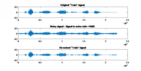
Figure 6. Time domain representation of clean, noisy and enhanced “Train” signals using modified ultraspherical window and RCGA
From the above tables, it is clear that the designed QMF banks using modified ultraspherical window and RCGA gives better performance in terms of PSNR and PESQ score compared to the Dolph-Chebyshev (As=60) and Kaiser (β=8) classical ultraspherical windows (μ=2, x0=1). Moreover, from Table 6 and 7 it can be observed that developed QMF banks gives better performances while compared to the classical algorithm based on wavelet detailed in the studies [25-27].
Figure 6 shows the time plot of clean test signal “Train.wav”, the noisy version corrupted by additive real noise and the denoised version using optimized QMF banks based on modified ultraspherical window. As it can be observed that the clean and enhanced signals are comparable.
In this work, modified ultraspherical window function is developed and exploited for designing efficient QMF banks with the help of real coded genetic. When designed QMF banks are used for speech enhancement algorithm based on wavelets techniques, the obtained simulation results prove that the modified ultraspherical window gives good performance in terms of PESQ and SNR compared with such window functions.
[1] Rajkumar, G., Jayabharathy, R., Narasimhan, K., Raju, N., Easwaran, M., Elamaran, V., Burbano-Fernandez, M. (2019). Spectral and SNR improvement analysis of normal and abnormal heart sound signals using different windows. Future Generation Computer Systems, 92: 438-443. https://doi.org/10.1016/j.future.2018.09.047
[2] Eleti, A.A., Zerek, A.R. (2013). FIR digital filter design by using windows method with MATLAB. In 14th International Conference on Sciences and Techniques of Automatic Control & Computer Engineering-STA'2013, pp. 282-287. https://doi.org/10.1109/STA.2013.6783144
[3] Takahashi, R., Suzuki, N., Tasaki, H. (2018). Window function for MIMO radar beamforming to mitigate multipath clutter. In 2018 International Conference on Radar (RADAR), pp. 1-6. https://doi.org/10.1109/RADAR.2018.8557234
[4] Molnar, G., Matijaščić, M. (2020). Window-to-polynomial transform and its application in antenna array design. In 2020 14th European Conference on Antennas and Propagation (EuCAP), pp. 1-5. https://doi.org/10.23919/EuCAP48036.2020.9135197
[5] Podder, P., Khan, T.Z., Khan, M.H., Rahman, M.M. (2014). Comparative performance analysis of hamming, Hanning and Blackman window. International Journal of Computer Applications, 96(18): 1-7.
[6] Kaiser, J.F. (1966). Digital filters. System Analysis by Digital Computer, 228-243.
[7] Peter, L. (1997). The Dolph–Chebyshev window: A simple optimal filter. American Meteorological Society, 125: 655-660.
[8] Avci, K., Nacaroglu, A. (2009). Cosh window family and its application to FIR filter design. AEU-International Journal of Electronics and Communications, 63(11): 907-916. https://doi.org/10.1016/j.aeue.2008.07.013
[9] Deczky, A.G. (2001). Unispherical windows. In ISCAS 2001. The 2001 IEEE International Symposium on Circuits and Systems (Cat. No. 01CH37196), 2: 85-88. https://doi.org/10.1109/ISCAS.2001.921012
[10] Saramaki, T. (1989). A class of window functions with nearly minimum sidelobe energy for designing FIR filters. In IEEE International Symposium on Circuits and Systems, pp. 359-362. https://doi.org/10.1109/ISCAS.1989.100365
[11] Kumar, A., Kuldeep, B. (2014). Design of cosine modulated pseudo QMF bank using modified Dolph-Chebyshev window. International Journal of Signal and Imaging Systems Engineering, 7(2): 126-133.
[12] Kumar, V., Bangar, S., Kumar, S.N., Jit, S. (2014). Design of effective window function for FIR filters. In 2014 International Conference on Advances in Engineering & Technology Research (ICAETR-2014), pp. 1-5. https://doi.org/10.1109/ICAETR.2014.7012964
[13] Kliewer, J., Brka, E. (2006). Near-perfect-reconstruction low-complexity two-band IIR/FIR QMF banks with FIR phase-compensation filters. Signal Processing, 86(1): 171-181. https://doi.org/10.1016/j.sigpro.2005.05.012
[14] Lee, J.H., Yang, Y.H. (2003). Design of two-channel linear-phase QMF banks based on real IIR all-pass filters. IEE Proceedings-Vision, Image and Signal Processing, 150(5): 331-338.
[15] Hu, Y., Loizou, P. (2007). Subjective comparison and evaluation of speech enhancement algorithms. Speech Communication, 49(7-8): 588-601. https://doi.org/10.1016/j.specom.2006.12.006
[16] Kuldeep, B., Kumar, A., Singh, G.K. (2015). Design of quadrature mirror filter bank using Lagrange multiplier method based on fractional derivative constraints. Engineering Science and Technology, an International Journal, 18(2): 235-243. https://doi.org/10.1016/j.jestch.2014.12.005
[17] Upendar, J., Gupta, C.P., Singh, G.K. (2010). Design of two-channel quadrature mirror filter bank using particle swarm optimization. Digital Signal Processing, 20(2): 304-313. https://doi.org/10.1016/j.dsp.2009.06.014
[18] Kumar, A., Singh, G.K., Anand, R.S. (2008). Near perfect reconstruction quadrature mirror filter. International Journal of Computer Science and Engineering, 2(3): 121-123.
[19] Bergen, S.W.A. (2005). Design of the ultraspherical window function and its applications. Thesis, B.Sc., University of Calgary.
[20] Deczky, A.G. (2001). Unispherical windows. In ISCAS 2001. The 2001 IEEE International Symposium on Circuits and Systems (Cat. No. 01CH37196), 2: 85-88. https://doi.org/10.1109/ISCAS.2001.921012
[21] Abramovich, F., Benjamini, Y. (1995). Thresholding of wavelet coefficients as multiple hypotheses testing procedure. In Wavelets and Statistics, 5-14. https://doi.org/10.1007/978-1-4612-2544-7_1
[22] Birgé, L., Massart, P. (1997). From model selection to adaptive estimation. In Festschrift for Lucien le Cam, 55-87. https://doi.org/10.1007/978-1-4612-1880-7_4
[23] Hu, Y., Loizou, P.C. (2004). Speech enhancement based on wavelet thresholding the multitaper spectrum. IEEE Transactions on Speech and Audio Processing, 12(1): 59-67. https://doi.org/10.1109/TSA.2003.819949
[24] Bhowmick, A., Chandra, M. (2017). Speech enhancement using voiced speech probability based wavelet decomposition. Computers & Electrical Engineering, 62: 706-718. https://doi.org/10.1016/j.compeleceng.2017.01.013
[25] Agbinya, J.I. (1996). Discrete wavelet transform techniques in speech processing. In Proceedings of Digital Processing Applications (TENCON'96), 2: 514-519. https://doi.org/10.1109/TENCON.1996.608394
[26] Zhong, X., Dai, Y., Dai, Y., Jin, T. (2018). Study on processing of wavelet speech denoising in speech recognition system. International Journal of Speech Technology, 21(3): 563-569. https://doi.org/10.1007/s10772-018-9516-7
[27] Cengiz, Y., Arıöz, Y.D.U. (2016). An application for speech denoising using Discrete wavelet transform. In 2016 20th National Biomedical Engineering Meeting (BIYOMUT), pp. 1-4. https://doi.org/10.1109/BIYOMUT.2016.7849377