Color Enhancement of Low Illumination Garden Landscape Images

After being converted to the luma-blue difference-red difference (YCbCr) color space, the original GLI is divided into multiple blocks. The mean value AV_o of Cr and mean value AV_e of Cb of each block are calculated. The cumulative absolute differences RP_o and RP_e of Cr and Cb of each block can be respectively calculated by:

$R P_{o}=\sum_{i, j}\left(\left|C_{r}(i, j)-A V_{o}\right|\right) / M$           (1)

$R P_{e}=\sum_{i, j}\left(\left|C_{b}(i, j)-A V_{e}\right|\right) / M$           (2)

The blocks with relatively small RP_o and RP_e are identified. These blocks should be removed, for they cannot provide sufficient color information. The mean values of AV_o, AV_e, RP_o and RP_e of the remaining blocks are taken as the AV_o, AV_e, RP_o and RP_e of the entire GLI. Next, the candidate set of white pixels can be judged and generated by:

$\begin{aligned}

&\left|C_{r}(i, j)-\left(A V_{o}+R P_{o} \times \operatorname{sign}\left(A V_{o}\right)\right)\right| \\

&<1.5 \times R P_{o}

\end{aligned}$           (3)

$\begin{aligned}

&\left|C_{b}(i, j)-\left(1.5 \times A V_{e}+R P_{e} \times \operatorname{sign}\left(A V_{e}\right)\right)\right| \\

&<1.5 \times R P_{e}

\end{aligned}$           (4)

The pixels with the top 10% brightness in the set are selected as the final white pixels. After that, all white pixels are adjusted. The first step is to compute the reference values of each white pixel in the three channels, i.e., the mean gray values of the three channels r_RV, g_RV, and b_RV. Next, the gain of each channel can be calculated by:

$\begin{aligned}

&r_{G}=Y_{\max } / r_{R V} \\

&g_{G}=Y_{\max } / g_{R V} \\

&b_{G}=Y_{\max } / b_{R V}

\end{aligned}$           (5)

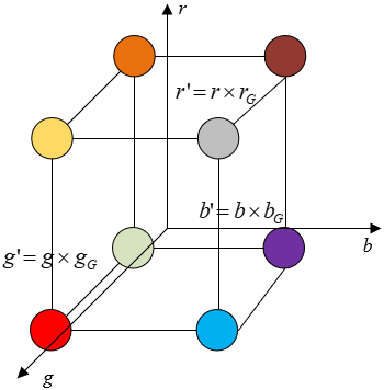
Based on the results of formula (5), the color values of the three channels of the GLI are modified by the framework shown in Figure 1. The pixels with color values surpassing the threshold can be identified by:

$\begin{aligned}

&r^{\prime}=r \times r_{G} \\

&g^{\prime}=g \times g_{G} \\

&b^{\prime}=b \times b_{G}

\end{aligned}$           (6)

For a GLI taken in a variable environment, if a single channel has a low gray value, then the mean gray value of that channel must be low, and the gain of that channel must be large. Through the abovementioned processing, the weak single-channel features could be compensated for.

1.png

Figure 1. Color correction framework

If the GLI has a small overall brightness, the Y value after color restoration will be relatively high, pushing up the overall brightness of the image. This will interfere with the judgement of candidate white pixels. To solve the problem, this paper introduces the attenuation offset parameter matrix ψ to quantify the dynamic threshold to a fixed range. The ψ depends on the photoelectric imaging environment. Based on this matrix, the Y, Cb and Cr of the original parameters are quantified again through the following derivation process:

$\left[\begin{array}{l}

Y^{\prime} \\

C_{b}{ }^{\prime} \\

C_{r}{ }^{\prime}

\end{array}\right]=W \cdot\left[\begin{array}{l}

Y \\

C_{b} \\

C_{r}

\end{array}\right]$           (7)

First, the attenuation of each color in the low illumination image is considered. Let ∫_ωγ^d(τ)dτ, ξ^d, and η^d be the vector integral, scattering coefficient, and attenuation coefficient of the light scattered into the sensor from all directions, respectively. The value of ∫_ωγ^d(τ)dτ is positively proportional to ξ^d. Since the global background light is a function of wavelength, we have:

$\gamma^{d}(\infty)=\frac{l_{k} l_{x}}{\eta^{d}} \int_{\omega} \gamma^{d}(\tau) d \tau$           (8)

where, l_k and S_x are constants. Let ξ(μ_d) be the reference wavelength scattering coefficient. Then, the linear relationship between scattering coefficient ξ^d and wavelength μ can be expressed as:

$\xi^{d}=\left(-0.00113 \mu_{d}+1.62517\right) \xi\left(\mu_{d}\right)$           (9)

Further, it can be derived that the global background light is proportional to ξ^d and inversely proportional to η^d:

$\gamma^{d}(\infty) \propto \frac{\xi_{\mu}}{\eta^{d}}$           (10)

The color channel with the smallest attenuation in the low illumination environment is defined as channel o. Based on the color attenuation of channel o, the attenuation ratio of any other color channel can be deduced as:

$\frac{\eta^{d}}{\eta^{o}}=\frac{\xi^{d} \gamma^{o}(\infty)}{\xi^{o} \gamma^{d}(\infty)} \quad d \in\{r, g\}$           (11)

The relationship between the attenuation ratios of the three channels can be expressed as:

$\begin{aligned}

&\sigma^{o}(a)=e^{-\delta(a)} \\

&\sigma^{d}(a)=\left(\sigma^{o}(a)\right)^{\frac{\eta^{d}}{\eta^{o}}} \quad d \in\{r, g\}

\end{aligned}$           (12)

Let W be the color space conversion matrix. According to the image transmission and display rules of the International Telecommunication Union (ITU), the RGB-YCbCr color space conversion can be expressed as:

$\begin{aligned}

&{\left[\begin{array}{c}

Y^{\prime} \\

C_{b}^{\prime} \\

C_{r}^{\prime}

\end{array}\right]=} \\

&{\left[\begin{array}{ccc}

0.3 & 0.59 & 0.12 \\

-0.17 & -0.33 & 0.5 \\

0.5 & -0.42 & -0.08

\end{array}\right] \cdot\left[\begin{array}{l}

R^{\prime} \\

G^{\prime} \\

B^{\prime}

\end{array}\right]=W \cdot\left[\begin{array}{l}

R^{\prime} \\

G^{\prime} \\

B^{\prime}

\end{array}\right]}

\end{aligned}$           (13)

The color space conversion matrix can be obtained based on the three-channel attenuation formulas:

$\left[\begin{array}{c}

R^{\prime} \\

G^{\prime} \\

B^{\prime}

\end{array}\right]=\left[\begin{array}{ccc}

\sigma^{r}(a) & & \\

& \sigma^{g}(a) & \\

& & \sigma^{b}(a)

\end{array}\right] \cdot\left[\begin{array}{c}

R \\

G \\

B

\end{array}\right]$           (14)

Combining formulas (13) and (14):

$\begin{aligned}

&{\left[\begin{array}{l}

Y^{\prime} \\

C_{b}^{\prime} \\

C_{r}^{\prime}

\end{array}\right]=W \cdot\left[\begin{array}{l}

R^{\prime} \\

G^{\prime} \\

B^{\prime}

\end{array}\right]} \\

&=W \cdot\left[\begin{array}{ll}

\sigma^{\prime}(a) & \\

& \sigma^{g}(a) & \\

& & \sigma^{b}(a)

\end{array}\right] \cdot\left[\begin{array}{l}

R \\

G \\

B

\end{array}\right]

\end{aligned}$           (15)

The color transformation of the original GLI can be expressed as:

$\left[\begin{array}{l}

Y \\

C_{b} \\

C_{r}

\end{array}\right]=W \cdot\left[\begin{array}{l}

R \\

G \\

B

\end{array}\right] \Rightarrow W^{-1} \cdot\left[\begin{array}{l}

Y \\

C_{b} \\

C_{r}

\end{array}\right]=\left[\begin{array}{l}

R \\

G \\

B

\end{array}\right]$           (16)

Substituting formula (16) into formula (15):

$\begin{aligned}

&{\left[\begin{array}{l}

Y^{\prime} \\

C_{b}^{\prime} \\

C_{r}^{\prime}

\end{array}\right]=W \cdot\left[\begin{array}{lll}

\sigma^{r}(a) & & \\

& \sigma^{g}(a) & \\

& & \sigma^{b}(a)

\end{array}\right]} \\

&W^{-1} \cdot\left[\begin{array}{l}

Y \\

C_{b} \\

C_{r}

\end{array}\right]=\psi \cdot\left[\begin{array}{l}

Y \\

C_{b} \\

C_{r}

\end{array}\right]

\end{aligned}$           (17)

The attenuation offset parameter matrix ψ can be derived by:

$\begin{aligned}

&\psi=W \cdot\left[\begin{array}{lll}

\sigma^{r}(a) & & \\

& \sigma^{g}(a) & \\

& & \sigma^{b}(a)

\end{array}\right] W^{-1} \\

&=W \cdot\left[\begin{array}{lll}

\left(\sigma^{o}(a)\right)^{\frac{\eta^{r}}{\eta^{o}}} & & \\

& \left(\sigma^{o}(a)\right)^{\frac{\eta^{g}}{\rho^{\circ}}} & \\

& & \left(\sigma^{o}(a)\right)^{\frac{\eta^{b}}{p^{\rho}}}

\end{array}\right] W^{-1}

\end{aligned}$           (18)

For the color channel with the least attenuation in the low illumination environment, the attenuation coefficient is assumed to satisfy η^d₌η^o. After this treatment, the single channel of the original GLI with a relatively low gray value can be compensated for, thereby balancing the gray value distribution across the three channels. The GLI color transform is illustrated in Figure 2.

2.png

Figure 2. GLI color transform

To verify the effectiveness of the proposed GLI color restoration algorithm, the performance of the modified dynamic threshold algorithms with and without ψ were quantified and analyzed. Table 1 presents the results of color cast detection based on equivalent circle, and evaluation results of GLI color quality.

The results show that the modified dynamic threshold algorithm with ψ outperformed that without ψ in GLI color restoration, evidenced by the relatively good restored color quality of all three types of GLIs (landscape architecture, landscape plants, and landscape water system). Despite a few color offsets in some images, the modified dynamic threshold algorithm with ψ perform excellently in the overall color restoration of GLIs. After enlarging the restored images, it can be found that some details of sculptures and artificial landscapes were better restored, and the color of water surfaces involving reflection/deflection was expressed accurately without over-exposure, after the modified dynamic threshold algorithm was coupled with ψ.

Table 1. Qualified evaluation of GLI color restoration

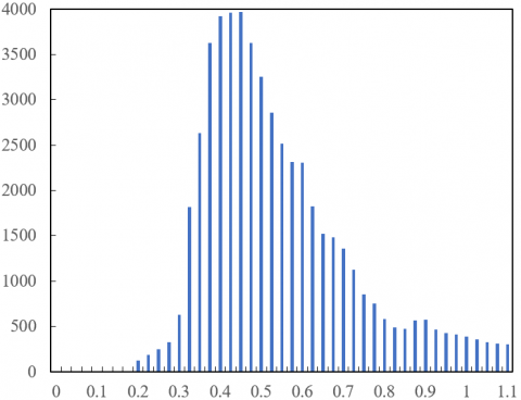
The histogram equalization simulation was carried out on GLIs captured in a low illumination environment. Figure 4 displays the histogram changes of the images before and after equalization.

4-1.png

(1) Before equalization

4-2.png

(2) After equalization

Figure 4. Histograms before and after introducing MAE loss and perpetual loss

Based on the principle of the color restoration and enhancement model and Figure 4, the CNN-based image enhancement of GLIs can be regarded as an approximate calculation process from continuous state to discrete state. As shown in Figure 4, the quantization error was small after introducing MAE loss and perpetual loss. As a result, there was a certain difference in the gray levels outputted by different gray pixel values after mapping. This effectively prevents the problems of traditional image enhancement methods: the merge of grayscales and the color information loss of GLIs. It can be intuitively seen from Figure 4 that, before introducing the MAE loss and perceptual loss, the pixels in the enhanced image were discretely distributed, and the histogram failed to retain the shape of the original image; after the two losses were introduced, the grayscale was uniformly distributed across the interval, and the histogram matched the shape of the original image.

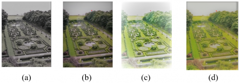
The restoration of the color information of the output GLI is greatly affected by the gain and offset of different values. By changing the size of the affine transformation parameters, it is possible to control the degree of color information restoration. Under the same experimental environment, a series of simulations were conducted with our algorithm, single-scale Retinex, and multi-scale Retinex. The color restoration results of these algorithms are compared in Figure 5.

5.png

Figure 5. Experimental results of color recovery of different algorithms

Figure 5 clearly displays that the GLI processed by our algorithm was much clearer, better in quality, and higher in brightness and contrast than that handled by single-scale Retinex, or multi-scale Retinex. By contrast, the image processed by single-scale Retinex had a low contrast, and that processed by multi-scale Retinex, and multi-scale was too white. The two contrastive algorithms fail to output realistic enhanced images that conform to our visual perception.

Tables 2-4 compare the quality of the GLIs enhanced by different algorithms. All three algorithms managed to enhance the color effect of the original GLIs. However, our algorithm was superior than the two traditional color enhancement algorithms, in terms of discrete entropy, clarity and contrast, and effectively improved the readability of low illuminance GLIs.

Table 2. Discrete entropy metric of each algorithm

Table 3. Clarity metric of each algorithm

Table 4. Contrast metric of each algorithm