Fengyun Cao
© 2021 IIETA. This article is published by IIETA and is licensed under the CC BY 4.0 license (http://creativecommons.org/licenses/by/4.0/).
OPEN ACCESS
Based on multi-feature fusion, this paper introduces a novel depth estimation method to suppress defocus and motion blurs, as well as focal plane ambiguity. Firstly, the node features formed by occlusion were fused to optimize image segmentation, and obtain the position relations between image objects. Next, the Gaussian gradient ratio between the defocused input image and the quadratic Gaussian blur was calculated to derive the edge sparse blur. After that, the fast guided filter was adopted to diffuse the sparse blur globally, and estimate the relative depth of the scene. Experimental results demonstrate that our method excellently resolves the ambiguity of depth estimation, and accurately overcomes the noise problem in real-time.
single defocused images, depth estimation, multi-feature fusion, edge sparse blur
In computer vision and image graphics, it is a key and basic problem to estimate the depth of three-dimensional (3D) scenes based on the limited clues of two-dimensional (2D) images. The depth of the scene can be applied in various fields, such as robotics, 3D reconstruction, image restoration, and image segmentation. After years of research and development, many algorithms have emerged for scene depth estimation.
The existing depth estimation algorithms rely on either monocular cues (vanishing points, shape, occlusion, texture change rate, etc.) [1, 2] or binocular cues (e.g., stereoscopic parallax). Traditionally, multiple images are needed to estimate the scene depth. For example, the stereo vision [3] and structure from motion [4] derive the scene depth from the geometric relationship between the corresponding feature points in two or more images. The depth from focus [5] measures the distance from the object point to the imaging system with the aid of a series of focused images that gradually become clearer. To estimate the scene depth, the conventional defocused distance measurement methods [6] iteratively change the setting of camera parameters, based on the blur degree of collected defocused images. However, this kind of methods are not widely applicable, owing to the complexity of feature matching and occlusion.
It is a challenging task to estimate the depth of single defocused images in uncalibrated cameras. The relevant algorithms have the following deficiencies: (1) Local edge blur is often measured inaccurately, and the edges are not extracted accurately, making it difficult to segment [7] the object; (2) The local blur diffusion is realized inefficiently by interpolation through image matting [8]; (3) Errors abound in the estimated scene depth.
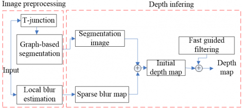
To solve the above deficiencies, this paper integrates multiple features [9], such as defocused blur, occlusion-based nodes, color, and texture, and develops a fast guided filter [10, 11] for global diffusion through the precise calculation of edge sparse blur, thereby improving the depth estimation. The proposed method can estimate the exact depth of the scene solely based on single defocused images from traditional cameras, without needing any additional condition. Therefore, the method is valuable in both theory and practice. The flow of our method is shown in Figure 1.
The main contributions of this work are as follows: Firstly, the focal plane ambiguity was effectively solved by introducing occlusion-based nodes. Secondly, blur estimation was combined with the fast guided filter to generate the depth map of a scene solely based on single defocused images from traditional cameras, without any modification to the camera or additional illumination. Thirdly, experimental results confirm the ability of our method to extract a layered depth map of the scene with a high accuracy.
Figure 1. Flow of our method
The remainder of this paper is organized as follows: Section 2 elaborates on the previous literature; Section 3 introduces the principle of defocus imaging, and the design of our method; Section 4 discusses the defocus blur and focal plane ambiguity, and carries out a comparative analysis through experiments; Section 5 the strengths and weaknesses of our method were summarized, and looks forward to future research.
The previous methods of scene depth estimation fall into two categories: (1) Traditional methods requiring constraints and prior knowledge; (2) Monocular estimation based on deep learning (DL). Currently, scene depth is mainly estimated by the above methods based on single images, with additional conditions, edge blur measurement, and multi-scale texture. Specifically, the additional conditions include the active lighting [12], and coded aperture [13]. But this kind of methods are severely constrained in actual practice, because of the need to attach specific light sources and modify the camera lens.
The research of texture information focuses on global, multi-scale, and hierarchical levels. For instance, Hoiem et al. [14] reconstructed 3D outdoor scenes referring to 3D geometric image textures. Despite achieving a good visual effect, their approach only applies to outdoor scenes, and deviates significantly from the actual depth. On this basis, Saxena et al. [15] applied machine learning (ML) to model the spatial relationship between outdoor objects, and estimate the depth of the outdoor scenes. But their algorithm involves massive computations, which undermines real-timeliness.
The typical strategies based on edge blur measurement are as follows: Starting with the non-uniform inverse heat conduction equation, Namboodiri and Chaudhuri [16] modeled image degradation as a thermal diffusion process. Hu and De Haan [17], and Zhuo and Sim [18] introduced edge matting and Markov random fields (MRF) to diffuse local blur graphs to global blur graphs, according to the linear relationship between defocused blur and depth. Drawing on methods like local consistency and over-segmentation, Shuai and Tong [19] and Cao et al. [20] and Bae and Frédo [21] proposed to spread local fuzziness of edges to global fuzziness. Nevertheless, their strategy divides the object that should fall in the same plane, resulting in excessive division of the input image and a high depth error.
In recent years, several DL applications have been developed for depth estimation, thanks to the growing computing power of graphics processing unit (GPU), and the explosion of image data. These applications can be primarily divided to supervised learning and unsupervised learning for absolute depth prediction. Eigen et al. [22] creatively applied deep neural network (DNN) to estimate monocular depth, and presented a multi-scale network, which predicts the global image depth with a coarse scale network, and optimizes the local details with a fine scale network. Eigen et al. [23] designed a general multi-scale network, which is applicable to depth estimation, surface normal estimation, and semantic labeling. Inspired by residual learning, Chen et al. [24] put forward a deep full convolution network (FCN), eliminating the need for postprocessing. Laina et al. [25] created an approach to naturally fuse the depth map predicted by convolutional neural network (CNN) with the depth map directly derived via monocular simultaneous localization and mapping (SLAM), and proved the excellence of the approach in low texture regions.
Owing to the supervision by the ground truth, the supervised learning methods above can effectively extract the depth information from single images. Nonetheless, their performance is limited by the labeled training sets, which are hard and expensive to acquire. Instead of using the costly ground truth, unsupervised learning methods [26-30] regard the geometric constraints between frames or binocular images as the supervisory signal for training.
3.1 Defocused image point degradation model
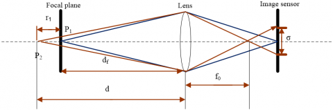
The scene target lies right at the focus, while the light converges on a clear point on the focal plane. If the target deviates from the focus, the light will converge to a blurred surface instead. The size of the blur area, which reflects the degree of blur, increases with the deviation, i.e., the image blur is positively correlated with the deviation. As shown in Figure 2, the radius r of the blur area can be calculated by:
$r=\frac{\left|d-d_{f}\right|}{d} \frac{f_{0}^{2}}{N\left(d_{f}-f_{0}\right)}$ (1)
where, f0 is the focal length; N is the range of camera aperture (f-number); d is the object distance.
Figure 2. Defocused image point degradation model
By fixing df and f0 and varying d and N, a nonlinear monotonic increasing relationship can be observed between the object distance and the radius of defocused blur. The relative depth of the scene can be estimated, once the defocused blur is available.
3.2 Local defocused bur estimation algorithms
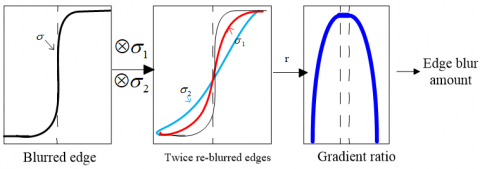
Hu and De Haan [17] were the first to estimate the edge local blur for defocused image restoration. Their algorithm applies quadratic Gaussian blur to an input defocused image, calculates the proportion difference between them, and performs a dot product operation with the edge graph, in order to obtain the edge sparse blur graph. Figure 3 shows the one-dimensional (1D) case of their algorithm: First, a step edge is re-blurred twice using a Gaussian function; then, the difference ratio is computed between the magnitude of the step edge and its two re-blurred versions; the amount of the defocus blur of an edge is measured, for the difference ratio maximizes in the edge regions.
Figure 3. Hu and De Haan [17] local blur estimation algorithm
On this basis, Fang et al. [19] implemented graph theory segmentation to obtain an over-segmentation graph; under the assumption of local consistency, the mean bur of several points in the segmentation block at the edge was fitted, and the fitted interpolation was propagated to the entire segmentation block via the line plane:
$d(i, j)=\frac{j_{\max }^{i}-j}{j_{\max }^{i}-j_{\min }^{i}} d\left(i, j_{\min }^{i}\right)+\frac{j-j_{\min }^{i}}{j_{\max }^{i}-j_{\min }^{i}} d\left(i, j_{\max }^{i}\right),(i, j) \in S_{n}$ (2)
where, Sn is the segmentation block;$j_{\max }^{i}$ and $j_{\min }^{i}$ are the maximum and minimum blurs of the j-th column in the block, respectively; $d\left(i, j_{\min }^{i}\right)$ and $d\left(i, j_{\max }^{i}\right)$ are the blurs of the leftmost and rightmost edges in the block, respectively. Finally, the sky area was modified separately, and the field depth was estimated with geometric constraints.
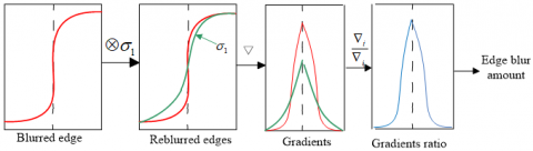
Zhuo and Sim [18] simplified the Hu and De Haan [17] quadratic Gaussian blur into a linear blur, and computed the gradient ratio with the input defocused image to obtain the maximum at the edge, before finally extracting the local edge blur (Figure 4).
Figure 4. Zhuo and Sim [18] local blur algorithm for Gaussian gradient ratio estimation
Note: $\otimes$ and $\nabla$ are convolution and gradient, respectively; black dotted lines are the edge positions.
(a) Original graph; (b) Results of Fang et al. [19]; (c) Actual depth
Figure 5. Example of depth errors
In Zhuo and Sim [18], the edge and defocused blur graphs are utilized in the dot product operation to produce the edge sparse blur graph. Then, the produced graph is propagated globally by the matting algorithm, in order to estimate the scene depth.
There are two disadvantages with Zhuo and Sim [18] and Fang et al. [19]: (1) The edge sparse blur does not contain the edge information reflecting the object in 3D scenes, which undermines the estimation performance of edge local blur. (2) The matting algorithm has a high time complexity in propagating local diffusion to the global scale. The diffusion of segmentation block is realized through graph theory segmentation. The resulting over-segmentation or over-merging brings a high error in depth estimation (Figure 5).
To overcome the disadvantages, this paper integrates T-junction clues to local blur estimation, and improves the accuracy of edge local blur, using the edge information obtained by an optimized segmentation. Next, a fast guided filter with a low time complexity was introduced to replace the matting algorithm for global diffusion, thereby optimizing the real-time performance.
3.3 Estimation of edge local defocused blur
The determination of local defocused blur requires highly accurate information about image edges. However, image edges are often positioned inaccurately under interferences like noise and texture details, making it difficult to extract the actual edges of an object in the scene. Inspired by the depth sorting of monocular images by occlusion nodes, this paper uses the cues of occlusion nodes to optimize image segmentation based on graph theory, and to reduce segmentation errors brought by over-segmentation or over-merging.
In graph-based segmentation [7], each image is regarded as an undirected graph:
$G=(V, E), v_{i} \in V$ (3)
where, V is the set of midpoints (image pixels) in the undirected graph; vi and vj are two pixels connected by an edge with weight w(vi,vj). Then, the segmentation result $w\left(v_{i}, v_{j}\right) \in E$ can be expressed as:
$S=\left\{\mathrm{C}_{i} \mid \mathrm{C}_{i} \in \mathrm{V}, \bigcup_{i} C_{i}=V, C_{i} \cap C_{j}=\varnothing_{i} \neq j\right\}$ (4)
where, Ci is the uncorrelated segmentation subset. Class interpolation can be defined as the difference among the elements in the same subset:
$\operatorname{Int}(C)=\max _{e \in M S T(C, E)} \quad w(e)$ (5)
where, MST (C, E) is corresponding to the minimum spanning tree of a segmentation subset C. The difference across segmentation subsets/classes can be expressed as:
$\operatorname{Diff}\left(C_{1}, C_{2}\right)=\min _{v_{i} \in C_{1}, v_{j} \in C_{2},\left(v_{i}, v_{j}\right) \in E}\quad w\left(\left(v_{i}, v_{j}\right)\right)$ (6)
Tunable segmentation results can be obtained by maximizing between-class difference, and minimizing in-class difference. The final output is controlled by three parameters: the value range of the minimum segmentation block (min_size), pre-segmentation Gaussian filtering and denoising parameter (σ), and between-class difference threshold (k), which varies with scene images and their sizes. If the k value is incorrect, over-segmentation or over-merging will easily occur, making it impossible to achieve accurate segmentation.
The over-segmentation strategy of Fang et al. [19] results in a high depth error, because objects in the same plane are segmented. As shown in Figure 5(b), depth errors exist on the road surface and buildings, both of which are over-segmented; trees cause the local blur diffusion to fail, and induce a serious deviation from the actual depth.
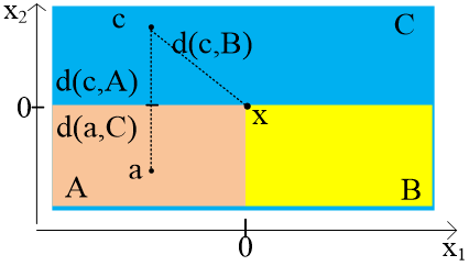
Figure 6 shows the structural relationship of T-junctions formed by object edge occlusion. The T-shaped junctions are formed as opaque objects A and B block object C. The common occlusion in image scenes is a key feature clue to derive monocular visual depth. In Figure 6, the fact that A is much closer to B than to C helps to solve focal plane ambiguity: The defocused blur graph only reflects the relative relationship between the focus plane and the objects in the scene, but cannot fully reflect the relative relationship among objects in the actual scene. In addition, the only known parameter is the distance between the object and the focus plane. But whether the object is in the front or rear of the focus plane remains unknown.
Figure 6. Structural relationship of T-junctions formed by object edge occlusion
The pixels $a \in A$ and $c \in C$ on the line vertical to the edges of objects A and C can be expressed as:
$Z(a)=0$ (7)
$Z(c)=e^{-\alpha|c|}\left(e^{\beta \frac{1}{|c| \gamma}}-1\right)$ (8)
where, $\alpha, \beta$ and $\gamma>0$. Then,
$Z(c)>Z(a)$ (9)
Similarly, it can be inferred that the c value of 3D coordinate z is greater than that of pixels a and b, i.e., it is farther away from the observer, resulting in a greater depth. The proof is available in Calderero and Caselles [9]. This paper records the T-junction position with the T-junction clue contained in the input image, judges the presence of a T-junction between the segmentation blocks, and determine whether the blocks should be merged.
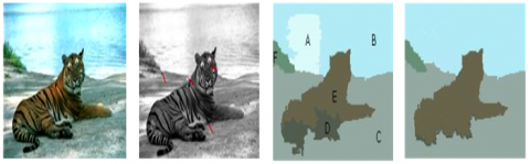
(a) Input image (b) T-junction clue image (c) Rough segmentation block (d) Regional merging
Figure 7. Optimal segmentation with regional merging based on T-junction clue
As shown in Figure 7, there is no T-junction in and between segmentation blocks A and B in the rough segmentation diagram, and regional merging exists. Block E has T-junctions but block D does not. There are T-junctions among blocks F, C, and A, without regional merging. After checking all the blocks, the final optimal segmentation graph was obtained, as well as the suitable object was segmented for scene depth estimation. In this way, the error induced by incorrect edges can be prevented, and the scene depth estimation can be more accurate than the local edge blur estimation of Zhuo and Sim [18] and Fang et al. [19].
In this paper, the local sparse blur amount is evaluated by Zhuo and Sim [18] method for local blur estimation with the Gaussian gradient ratio. Given that the blurred edge is blurred again by the Gaussian blur kernel with a known standard deviation, the gradient ratio of the original blur edge to the twice blurred edge was solved, and the maximum ratio was taken as the local defocused blur at the edge. For simplicity, the estimation of edge sparse blur is described in the 1D case (Figure 4). After the second blur, the gradient at the edge of the input image can be calculated by:
$\nabla i_{1}(x)=\nabla\left((A u(x)+B) \otimes g(x, \sigma) g\left(x, \sigma_{1}\right)\right) =\frac{A}{\sqrt{2 \pi\left(\sigma^{2}+\sigma_{1}^{2}\right)}} \exp \left(\frac{x^{2}}{2\left(\sigma^{2}+\sigma_{1}^{2}\right)}\right)$ (10)
where, $\sigma_{l}$ is the standard deviation of the quadratic blur Gaussian kernel, i.e., the degree of blur. The edge gradient ratio of the input image to the quadratic blurred image can be established as:
$\frac{|\nabla i(x)|}{\left|\nabla i_{1}(x)\right|}=\sqrt{\frac{\sigma^{2}+\sigma_{1}^{2}}{\sigma^{2}}} \exp \left(\frac{x^{2}}{2 \sigma^{2}}-\frac{x^{2}}{2\left(\sigma^{2}+\sigma_{1}^{2}\right)}\right)$ (11)
The maximum ratio can be obtained at the position (x=0) of the edge. The maximum R can be expressed as:
$R=\frac{|\nabla i(0)|}{\left|\nabla i_{1}(0)\right|}=\sqrt{\frac{\sigma^{2}+\sigma_{1}^{2}}{\sigma^{2}}}$ (12)
Formulas (10) and (11) imply that the edge gradient mainly depends on the amplitude A and the blur kernel σ, while the maximum gradient ratio R is independent of amplitude A and solely dependent on σ and σ1. Therefore, the blur kernel σ of the unknown input defocused image can be calculated from the R value and the known σ1 value of the structure:
$\sigma=\frac{1}{\sqrt{R^{2}-1}} \sigma_{1}$ (13)
The blur of 2D images can be estimated in a similar manner. Taking the 2D Gaussian blur kernel σ1=5, the gradient can be calculated by:
$\|\nabla i(x, y)\|=\sqrt{\nabla i_{x}^{2}+\nabla i_{y}^{2}}$ (14)
where, $\nabla i_{x}$ and $\nabla i_{y}$ are the gradients along x- and y-axes, respectively. Figure 8 compares the edge sparse blur graph extracted by Zhuo and Sim [18] and that extracted by our method.
(a) Input image (b) Zhuo and Sim’s [18] results (c) Our results
Figure 8. Edge sparse blur estimation
Zhuo and Sim [18] used the matting algorithm to propagate local blur to global blur, get the global blur graph, and estimate the scene depth according to the nonlinear monotone increasing relationship between defocused blur and depth. The core of the diffusion method can be expressed as:
$E(\mathrm{~d})=d^{T} L d+\lambda(d-\hat{d})^{T} D(d-\hat{d})$ (15)
where, d is the global blur graph; $\hat{d}$ is the edge local blur graph; L is the matting Laplacian matrix; D is the diagonal matrix; λ is the parameter to balance the accuracy of the local blur graph with the smoothness of the global blur graph.
By contrast, this paper employs a fast guided filter similar to the matting algorithm. Through guided filtering, the fast guided filter reduces the number the pixels by down-sampling the guide and input graphs. Hence, the time complexity can be reduced O(N) to $O\left(\frac{N}{s^{2}}\right)$, where s is the ratio of down-sampling. If s = 4, the algorithm will be accelerated by more than 10 times.
For the i-th pixel in the global blur graph, the diffusion can be expressed as:
$d_{i}=\sum_{j} W_{i j}(F) \hat{d}$ (16)
where, F is the guide image, i.e., the original defocused image; Wij is the filter kernel function:
$W_{i j}(I)=\frac{I}{|\omega|^{2}} \sum_{k(i, j) \in \omega_{k}}\left(I+\frac{\left(I_{i}-\mu_{k}\right)\left(I_{j}-\mu_{k}\right)}{\sigma_{k}^{2}+\varepsilon}\right)$ (17)
where, ωk is the k-th kernel function window; $|\omega|$ is the number of the pixels in that window; $\mu_{k}$ and $\sigma_{k}^{2}$ are the mean and variance, respectively; ε is the smoothing factor.
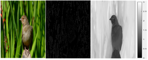
In practical applications, a scene is either a simple indoor scene or a complex natural scene. Multiple groups of images with the two types of scenes were selected for a series of comparative experiments between our method with other baselines. The effectiveness of our method was verified by the experimental results. The depth recovery results of our method are reported in Figure 9, where subgraph (a) gives the input image; subgraph (b) shows the edge sparse bur of the input image; (c) presents the relative scene depth amplified by our method. The edge sparse bur is negatively correlated with the distance. For instance, the bird in Figure 9 is a close view and the background is a long view. As shown in subgraph (d), the color scale of the results of our method ranged from 0 to 3, i.e., the relative depth of the scene trended from near to far. The experimental parameters are mentioned in previous sections.
(a) Input image (b) Edge sparse blur (c) Depth map (d) Color bar
Figure 9. Depth recovery result of our method
4.1 Comparison of blur texture ambiguity
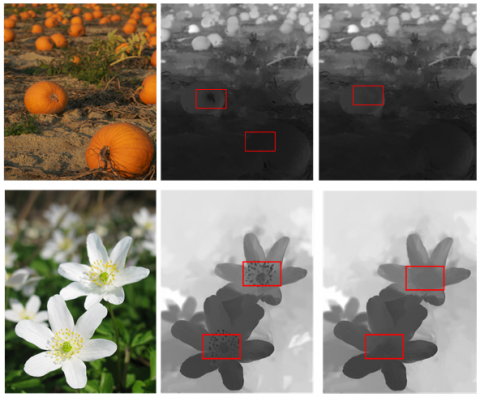
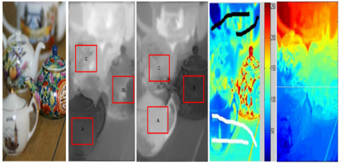
Figure 10 compares our method with Zhuo and Sim [18]. The first group of experimental results shows that the depth of the target scene trended gradually from bottom to top, while the second group suggested that the depth changed gradually from flowers to the background. The position of the red rectangle should be in the same plane, and the depth should be the same within the rectangle. However, Zhuo and Sim [18] faced a depth error due to the blur texture ambiguity. This error was overcome by our method, which obtains the edge information accurately. Our method also outperformed the contrastive algorithm in efficiency, because it discards the time-consuming matting algorithm.
(a) Input image (b) Results of Zhuo and Sim [18] (c) Results of our algorithm
Figure 10. Comparison of depth recovery by different methods
4.2 Comparison of focal plane ambiguity
Figure 11 compares our method with Zhuo and Sim [18], and Cao et al. [20] in the experiment on the simple desktop scene. The comparison confirms the effectiveness of our method, which handles focal plane ambiguity by changing the focus position. Zhuo and Sim [18] algorithm solved the problem by focusing on the nearest or farthest point during image acquisition. The rectangular boxes show that teapots A and C deviated from the focal plane by the same distance. At this moment, Zhuo and Sim [18] could not determine whether the teapots are before or behind the focal plane, or estimate the exact depth. Cao et al. [20] solved this problem with user-specified near-focus and far-focus areas. In our method, the optimal segmentation merges the various node features formed by occlusion to reveal the relative position between objects, and thus solves the ambiguity of the focal plane, as indicated by Figure 11(c).
(a) Input image (b) Results of Zhuo and Sim [18] (c)Results of our algorithm (d) Image with user-defined foreground (white strokes) and background (black strokes) prepared by Cao et al. [20] (e) Results of Cao et al. [20]
Figure 11. Comparison of simulated position changes of focal plane
4.3 Other comparisons
Figure 12 compares our method with Zhuo and Sim [18], which is based on the matting algorithm. The matting process makes the contrastive algorithm consume much more time, and produce more halo artifacts than our method. On bird and flower images, Zhuo and Sim [18] made mistakes in differentiating the foreground from the background (marked by the box). On the building image, the scene can be divided into 3 layers: Walls, buildings, and sky. The focus is on the wall in the foreground. Our method effectively restored the panoramic depth map of the scene (subgraph (c)): all the three layers were included, and placed from near to far. On the contrary, Zhuo and Sim [18] had obvious depth errors in positioning the sky.
(a) Input image (b) Results of Zhuo and Sim [18] (c) Results of our algorithm
Figure 12. Comparison of depth recovery results by different algorithms
Figure 13 further compares our method with Bae et al. [21], Zhuo and Sim [18], and Cao et al. [20]. The depth maps of Cao et al. [20], Zhuo and Sim [18], and Bae et al. [21] were not satisfactory, in which some focused regions were destroyed, and some were not blurred adequately, e.g. the hair and the clothes. In contrast, our results were visually closer to the truth.
(a) Input image (b) Results of Bae et al. [21] (c) Results of Cao et al. [20] (d) Results of Zhuo and Sim [18] (e) Results of our algorithm
Figure 13. Comparison of depth recovery results from different algorithms
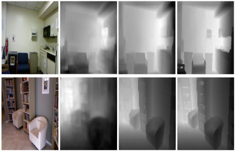
To further verify the effectiveness of our method, quantitative experiments were carried out to compare the algorithm with the latest DL model [22, 24], using the NYU-Depth Dataset [22]. The dataset consists of indoor scenes with ground-truth Kinect depth. As shown in Figure 14, the depth map of our method had much more refined contours than that of Eigen et al.’s algorithm [22].
(a) Input image (b) Results of Eigen et al. [22] (c) Results of our algorithm (d) Ground truth
Figure 14. Qualitative results of different methods on NYU Depth
Note: All depth maps except ours are directly from [22].
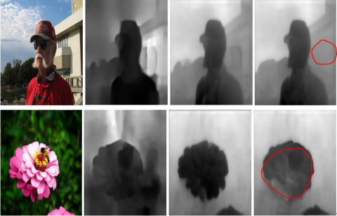
(a) Input image (b) Results of Eigen et al. [22] (c) Results of Chen et al. [24] (d) Results of our algorithm
Figure 15. Qualitative results of different methods on DIW dataset
Finally, our method was compared with Eigen et al. [22], and Chen et al. [24] on the famous Wild (DIW) dataset. As Shown in Figure 15, the contours in the depth map of our method were more refined than those in the depth map of Eigen et al.’s algorithm, and Chen et al.’s algorithm. Of course, some defects appeared when the depth surpassed 10m. In this case, estimation error was observed in the corresponding region, calling for further research.
The quantitative evaluation manifested that supervised DL is superior in the scenes with a large depth of field, and able to obtain real depth values with a high accuracy. However, DL algorithms require lots of labeled image sets with diverse scenes. The acquisition of such image sets would be costly and time-consuming.
This paper proposes a depth estimation method based on multi-feature fusion. Specifically, the Gaussian gradient ratio was adopted to estimate the local sparse blur at the edge extracted from feature clues in the input image. Moreover, the fast guide filter was called for global diffusion of the local sparse blur to produce accurate global blur graphs, and recover the depth of the target scene. By fusing defocused information, color information, texture, and occlusion cues, our method satisfactorily solves defocus and motion blurs, as well as focal plane ambiguity in depth estimation. Particularly, our method achieves an outstanding efficiency by eliminating the high computing load in deconvolution and matting operations of former algorithms. The effectiveness and robustness of our method are fully demonstrated through a series of comparative experiments.
Although our method solves the ambiguity of blur texture and focal plane, it may fail in many scenes under the specific assumption of local defocus. More importantly, this method is limited to deriving the relative depth of the scene. The DL has become a mainstream technique, with the leapfrog development of GPU and continuous improvement of computing power. In future research, the other types of limited information will be integrated to the current DL algorithms, aiming to expand our method to other fields.
This work was supported by Anhui Province University Excellent Talent Support Program Project, No. gxyq2019068. Anhui Province Key Laboratory of Simulation and Design for Electronic Information System (Hefei Normal University), No. 2019ZDSYSZY06. The Open Project of Anhui Provincial Key Laboratory of Multimodal Cognitive Computation, Anhui University, No. MMC202009.
[1] Akbarally, H., Kleeman, L. (1996). 3D robot sensing from sonar and vision. In Proceedings of IEEE International Conference on Robotics and Automation, 1: 686-691. https://doi.org/10.1109/ROBOT.1996.503854.
[2] Stephen, T., Martin, A. (1982). Computational stereo. ACM Computing Surveys, 14(4): 553-572. https://doi.org/10.1145/356893.356896
[3] Scharstein, D., Szeliski, R. (2002). A taxonomy and evaluation of dense two-frame stereo correspondence algorithms. International Journal of Computer Vision, 47(1): 7-42. https://doi.org/10.1109/SMBV.2001.988771
[4] Favaro, P., Soatto, S. (2005). A geometric approach to shape from defocus. IEEE Transactions on Pattern Analysis and Machine Intelligence, 27(3): 406-417. https://doi.org/10.1109/TPAMI.2005.43
[5] Favaro, P., Soatto, S., Burger, M., Osher, S.J. (2008). Shape from defocus via diffusion. IEEE Transactions on Pattern Analysis and Machine Intelligence, 30(3): 518-531. https://doi.org/10.1109/TPAMI.2007.1175
[6] Zhou, C., Cossairt, O., Nayar, S. (2010). Depth from diffusion. In 2010 IEEE Computer Society Conference on Computer Vision and Pattern Recognition, pp. 1110-1117. http://doi.org/10.1109/CVPR.2010.5540090
[7] Felzenszwalb, P.F., Huttenlocher, D.P. (2004). Efficient graph-based image segmentation. International Journal of Computer Vision, 59(2): 167-181. https://doi.org/10.1023/B:VISI.0000022288.19776.77
[8] Levin, A., Lischinski, D., Weiss, Y. (2007). A closed-form solution to natural image matting. IEEE Transactions on Pattern Analysis and Machine Intelligence, 30(2): 228-242. https://doi.org/10.1109/TPAMI.2007.1177
[9] Calderero, F., Caselles, V. (2013). Recovering relative depth from low-level features without explicit T-junction detection and interpretation. International Journal of Computer Vision, 104(1): 38-68. https://doi.org/10.1007/s11263-013-0613-4
[10] He, K., Sun, J. (2015). Fast Guided Filter. Computer Science. https://arxiv.org/abs/1505.00996v1.
[11] He, K., Sun, J., Tang, X. (2012). Guided image filtering. IEEE Transactions on Pattern Analysis and Machine Intelligence, 35(6): 1397-1409. https://doi.org/10.1109/TPAMI.2012.213
[12] Moreno-Noguer, F., Belhumeur, P.N., Nayar, S.K. (2007). Active refocusing of images and videos. ACM Transactions On Graphics (TOG), 26(3): 67-es. https://doi.org/10.1145/1275808.1276461
[13] Levin, A., Fergus, R., Durand, F., Freeman, W.T. (2007). Image and depth from a conventional camera with a coded aperture. ACM Transactions on Graphics (TOG), 26(3): 70-es. https://doi.org/10.1145/1276377.1276464
[14] Hoiem, D., Efros, A.A., Hebert, M. (2005). Geometric context from a single image. In Tenth IEEE International Conference on Computer Vision (ICCV'05), 1: 654-661. https://doi.org/10.1109/ICCV.2005.107
[15] Saxena, A., Sun, M., Ng, A.Y. (2008). Make3d: Learning 3d scene structure from a single still image. IEEE Transactions on Pattern Analysis and Machine Intelligence, 31(5): 824-840. https://doi.org/10.1109/TPAMI.2008.132
[16] Namboodiri, V.P., Chaudhuri, S. (2008). Recovery of relative depth from a single observation using an uncalibrated (real-aperture) camera. In 2008 IEEE Conference on Computer Vision and Pattern Recognition, pp. 1-6. https://doi.org/10.1109/CVPR.2008.4587779
[17] Hu, H., De Haan, G. (2006). Low cost robust blur estimator. In 2006 International Conference on Image Processing, pp. 617-620. https://doi.org/10.1109/ICIP.2006.312411
[18] Zhuo, S., Sim, T. (2011). Defocus map estimation from a single image. Pattern Recognition, 44(9): 1852-1858. https://doi.org/10.1016/j.patcog.2011.03.009
[19] Fang, S., Qin, T., Cao, Y., Cao, F.Y. (2013). Depth recovery from a single defocused image based on depth locally consistency. In Proceedings of the Fifth International Conference on Internet Multimedia Computing and Service, pp. 56-61. https://doi.org/10.1145/2499788.2499836
[20] Cao, Y., Fang, S., Wang, Z. (2013). Digital multi-focusing from a single photograph taken with an uncalibrated conventional camera. IEEE Transactions on Image Processing, 22(9): 3703-3714. https://doi.org/10.1109/TIP.2013.2270086
[21] Bae, S., Frédo D. (2010). Defocus magnification. Computer Graphics Forum, 26(3): 571-579. https://doi.org/10.1111/j.1467-8659.2007.01080.x
[22] Eigen, D., Puhrsch, C., Fergus, R. (2014). Depth map prediction from a single image using a multi-scale deep network. arXiv preprint arXiv:1406.2283
[23] Eigen, D., Fergus, R. (2015). Predicting depth, surface normals and semantic labels with a common multi-scale convolutional architecture. In Proceedings of the IEEE International Conference on Computer Vision, pp. 2650-2658. https://doi.org/10.1109/ICCV.2015.304
[24] Chen, W., Fu, Z., Yang, D., Deng, J. (2016). Single-image depth perception in the wild. Advances in Neural Information Processing Systems, 29: 730-738. https://doi.org/10.5555/3157096.3157178
[25] Laina, I., Rupprecht, C., Belagiannis, V., Tombari, F., Navab, N. (2016). Deeper depth prediction with fully convolutional residual networks. In 2016 Fourth International Conference on 3D Vision (3DV), pp. 239-248. https://doi.org/10.1109/3DV.2016.32
[26] Tateno, K., Tombari, F., Laina, I., Navab, N. (2017). Cnn-slam: Real-time dense monocular slam with learned depth prediction. In Proceedings of the IEEE Conference on Computer Vision and Pattern Recognition, pp. 6243-6252. https://doi.org/10.1109/CVPR.2017.695
[27] Garg, R., Bg, V.K., Carneiro, G., Reid, I. (2016). Unsupervised CNN for single view depth estimation: Geometry to the rescue. In European Conference on Computer Vision, pp. 740-756. https://doi.org/10.1007/978-3-319-46484-8_45
[28] Godard, C., Mac Aodha, O., Brostow, G.J. (2017). Unsupervised monocular depth estimation with left-right consistency. In Proceedings of the IEEE Conference on Computer Vision and Pattern Recognition, pp. 270-279. https://doi.org/10.1109/CVPR.2017.699
[29] Amiri, A.J., Loo, S.Y., Zhang, H. (2019). Semi-supervised monocular depth estimation with left-right consistency using deep neural network. In 2019 IEEE International Conference on Robotics and Biomimetics (ROBIO), pp. 602-607. https://doi.org/10.1109/ROBIO49542.2019.8961504
[30] Zhou, T., Brown, M., Snavely, N., Lowe, D.G. (2017). Unsupervised learning of depth and ego-motion from video. In Proceedings of the IEEE Conference on Computer Vision and Pattern Recognition, pp. 1851-1858. https://doi.org/ 10.1109/CVPR.2017.700