Rabah Hamdini* | Nacira Diffellah | Abderrahmane Namane
© 2021 IIETA. This article is published by IIETA and is licensed under the CC BY 4.0 license (http://creativecommons.org/licenses/by/4.0/).
OPEN ACCESS
In the last few years, there has been a lot of interest in making smart components, e.g. robots, able to simulate human capacity of object recognition and categorization. In this paper, we propose a new revolutionary approach for object categorization based on combining the HOG (Histograms of Oriented Gradients) descriptors with our two new descriptors, HOH (Histograms of Oriented Hue) and HOS (Histograms of Oriented Saturation), designed it in the HSL (Hue, Saturation and Luminance) color space and inspired by this famous HOG descriptor. By using the chrominance components, we have succeeded in making the proposed descriptor invariant to all lighting conditions changes. Moreover, the use of this oriented gradient makes our descriptor invariant to geometric condition changes including geometric and photometric transformation. Finally, the combination of color and gradient information increase the recognition rate of this descriptor and give it an exceptional performance compared to existing methods in the recognition of colored handmade objects with uniform background (98.92% for Columbia Object Image Library and 99.16% for the Amsterdam Library of Object Images). For the classification task, we propose the use of two strong and very used classifiers, SVM (Support Vector Machine) and KNN (k-nearest neighbors) classifiers.
categorization, descriptor, HOG, HSL, KNN, recognition, robots, SVM
In computer vision, we have to differentiate two words, categories of objects (associated with shapes) and instances of objects (associated with things). Bicycles and computers are examples of categories of objects. While the red bicycle and a Toshiba A-610 computer are instances of objects. Two tasks are associated with object recognition, the first task is object detection, i.e., we aim to detect a class of objects e.g. detecting the class of bicycle (similar bicycles), the second is the categorization of objects, i.e. we aim to differentiate instances of objects of the same class i.e. differentiate two bicycles similar, the first is red and the other blue, the last is the segmentation of objects.
For humans, seeing is an innate task and we often do not measure the difficulty in artificially obtaining the same performance. While in computer vision, and despite advances, the systems developed are far from equaling the performance of the human eye and brain. One of the best ways to give smart components this categorization ability is to use histograms.
The colors of objects and their visual appearances have been the subject of great interest and receive special attention in various industrial and commercial activities. There are many methods that use color signatures for the recognition and categorization of objects. Among these, we can cite the methods based on the modeling of histograms [1, 2], on the correlation of wavelets [3], on the co-occurrence matrices [4, 5], on the color moments [6-8] and many others (Markov fields [9], color coherence vectors [10], color correlogram [11]).
The histograms (or distributions) are a diagram made up of rectangles whose area is proportional to the frequency of a variable and whose width is equal to the class interval. These distributions are very varied in image processing: color histograms, spatial histograms and combined histograms. The first histogram to be developed is the HOI (Histogram of Intensity). It is part of the color histograms; it consists of recording the number of pixels for each intensity (in a class by intensity) in a specific region of the image. HOI is a translation and rotation invariant descriptor [12]. It is also very small compared to the region initially analyzed [12]. HOI then became more complex to adapt to the color. Developments in color accelerated in the 1990s.
The histogram methods have been used a lot in relation to a spatial character. Among them, three major descriptors can be cited: the co-occurrence matrix, the Shape Context and the HOG. The co-occurrence matrix was proposed in 1973 to analyze textures. This method was most widely used in the thirty years following its publication [13]. Although this method is used much less in the context of colored objects, this type of method nevertheless remains interesting for the description. A co-occurrence matrix is a form of 2D histogram. First, a displacement vector (orientation and spatial distance) is defined. The co-occurrence matrix then records the number of pairs of pixels as a function of the difference in their intensity and according to the given displacement vector. The moments on this matrix are then calculated. It should be noted that these measures could lead to classifying this descriptor in the category of statistical descriptors based on moments. The shape context descriptor is also based on a spatial count. However, it has two differences with the co-occurrence matrix. First of all, the counting is no longer done according to the intensities but according to the directions and the radius (according to a diagram in polar coordinates). Indeed, the form context consists in creating classes, or bins, in a circular format. Then, the counted value is the amount of outline type pixels in each area of the histogram. For each class, the number of points forming part of a contour is counted. This describes the local form of an object.
HOG was first proposed in 2004 by Lowe [14] in the SIFT (Scale Invariant Feature Transform) image association algorithm as a descriptor. This method was then used in 2005 by Dalal [15, 16] as a descriptor for the classification of pedestrians. This descriptor will be presented in section 2.1.
The MPEG-7 (Moving Picture Experts Group) standard [17] also offers a descriptor of this type: the Color Structure Descriptor (CSD). The CSD is a 1D histogram, each class of this histogram corresponds to a color and records the number of structuring elements (from a predefined set) for which the color is present in the structuring element (by applying it as a mask to the image).
More recent descriptors combine spatial and colorimetric distributions. The color correlogram descriptor is a 2D histogram that records the number of occurrences in which two pixels of the same color are at a given distance. There is therefore a class for each color-distance pair. In this descriptor, the direction between the two pixels is not taken into account, unlike the co-occurrence matrix.
Maggio et al. [18] proposed an appearance model based on the combination of the weighted color histogram and the gradient orientation histogram. A target object is approximated by an ellipse. For the color histogram, an elliptical kernel is applied to favor pixels near the center. Then the color histogram is normalized. A probability vector is thus obtained for each histogram. It is integrated into a monitoring process based on the particle filter algorithm.
Another similar approach has been developed by Yan et al. [19], the authors proposed an appearance model by combining several characteristics, namely the color histogram, the movement characteristics (including the speed of movement, the scale of the object and the angle of displacement objects) and optical flow (the histogram of motion based on the amplitude and angle of the optical flow vector). Each similarity score obtained by one of these characteristics is weighted by a weight in order to calculate the overall similarity score. The weight is determined by a discriminating learning process.
The target object is described using: the color histogram, the covariance matrices and the HOG gradient histogram [20]. The combination of these descriptors is done using the adaboost algorithm.
All these systems aim to predict the nature of the object in an image from an exhaustive list of possibilities. In our last work [21], we proposed an object categorization model based only on the colors of the objects. After a while, we noticed that this model is less effective in an environment where there are a lot of objects with close or similar colors. Therefore, to improve the result of this model, in this article we decided to separate the hue and saturation values to make the model more able to distinguish colors. In addition, we decided to associate the color of the object with its shape (outlines) to improve the ability of this model to distinguish objects that have close or similar colors. In this paper, we propose a new object categorization algorithm designed in the HSL color space, which closely approximates the physiological perception of color by the human eye, and based on the use of ideas of cells and bins used in the HOG descriptor. All of this combination produces results that we consider revolutionary in the world of object recognition and categorization.
This article is organized as follows: In section 2, we present some old methods of object recognition and categorization in order to compare their results with the results of the proposed methods. In section 3, we start by presenting the HSL color space and its performances which justify the choice of this color representation model, then we move on to explain the construction steps of the proposed descriptor. Section 4 is an overview of KNN and SVM. Finally, the results of the various experiments carried out on Columbia Object Image Library (COIL-100) and The Amsterdam Library of Object Images (ALOI) are shown in section 5.
In this section, we first define, in brief, the main photometric and geometric changes. Then, we move on to present the existing methods that will be used in a comparative study in section 5. These methods will be cited in chronological order, starting with the descriptor HOG, followed by opponent histograms, hue histograms and we end with our last published work, the hue descriptor.
While the geometric changes involve the placement of objects (e.g., translation, rotation, angle of view), but do not affect the shape of the objects nor their topology, in short, photometric changes content:
—Shadows and lighting geometry changes such as shading, it’s the light intensity changes.
—Scattering of a white source and object highlights under a white light source, its light intensity shifts.
—The combinations of the above two conditions, the light intensity changes and shifts.
—Scattering and a change in the illumination color, it’s the light color change.
—Object highlights under an arbitrary light source and changes in the illumination, as above, it’s the light color change and shift.
For additional details and derivations, we refer to the study [22].
2.1 HOG (Histogram of Oriented Gradient)
The descriptor HOG, largely inspired by SIFT, was proposed by Dalal and Triggs in 2005 to respond to the limitations of SIFT [14] in the case of dense grids [15, 16]. The main idea of this descriptor is that the local structure of the object is characterized by calculating the distribution of the gradients of the local intensities or of the directions of the contours, without having a prior knowledge of the localization of the gradient or of the position of the contours of the object in the image.
The image is divided into a set of adjacent regions of fixed size, called blocks. For each block, we calculate a local 1D histogram of gradient direction or contour orientation: the values were estimated by performing a Gaussian smoothing followed by the application of a simple 1D mask of derivatives [-1; 0; 1] at scale 0. Thus, the HOG descriptor is calculated by a simple concatenation of the orientation histograms of the block gradients with nine orientations considered. To avoid the side effect produced by the orientation of the blocks, a bilinear interpolation was made between the neighborhoods of each block. In the case of color images, the gradients are calculated for each color channel and we just consider those which have the standard closest to the gradient vectors calculated at the pixel level. Finally, to make this descriptor robust to changes in illumination and contrast, L2 or L1 type normalization was carried out [15, 16].
2.1.1 HOG normalization
Four types of normalization are explored [15, 16]. Let v be the non-normalized vector containing all histograms in a given block, $\|v\|_{k}$ be its $\mathrm{k}$-norm for $k=1,2, \ldots$ and $e$ be some small constant (the exact value, hopefully, is unimportant). The normalization factor is then defined by:
L2-norm: $f=\frac{v}{\sqrt{\left\| v \right\|_{2}^{2}+{{e}^{2}}}}$ (1)
L1-norm: $f=\frac{v}{\left( {{\left\| v \right\|}_{1}}+{{e}^{2}} \right)}$ (2)
L1-root: $f=\sqrt{\frac{v}{\left( {{\left\| v \right\|}_{1}}+{{e}^{2}} \right)}}$ (3)
A fourth norm L2-hys, consisting of calculating v first by the L2-norm, then limiting the maximum of v values to 0.2, and then doing a renormalizing.
2.1.2 Hog limitations and proposed solutions
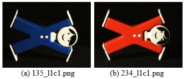
Since the HOG descriptor was proposed, several recognition systems have used it and they have shown very good performance, which has rekindled interest in dense un-quantized descriptors. HOG features are offered for the detection of pedestrians (humans) and later many researchers used them to detect other objects such as cars, dogs, cats, etc. In this article, and for the first time since it appeared, we aim to use this feature in the categorization of colorful handmade objects. The main problem in this type of categorization is to make the HOG able to distinguish objects that have the same shape and the same outlines, therefore the same tangent arc, but with different colors (Figure 1).
Figure 1. Two objects from the ALOI dataset with the same contours and different colors
To solve this difficult distinction problem, as well as the problems of missing invariance to photometric and geometric changes, we propose to add successively two other descriptors to the hog called HOH (Histogram of oriented hue) and HOS (Oriented saturation histogram). The final feature of the object will be the combination of these three descriptors (HOH, HOS and HOG). The details and advantages of this combination will be presented in section 3.
2.2 Hue histograms
In the HSV color space, hue and saturation values are given by:
$hue=\arctan \left( \frac{\sqrt{3}\left( R-G \right)}{R+G-2B} \right)$ (4)
$saturation=\sqrt{\frac{2}{3}\left( {{R}^{2}}+{{G}^{2}}+{{B}^{2}}-RG-RB+GB \right)}$ (5)
R is the red component of images in RGB color space, G is the green one and B represents the bleu component.
The hue histogram [23] is a 1D histogram designed for regions of interest and based on the hue channel of the HSV color space. It is obtained by weighing the distance between each hue sample at the center of the region of interest, samples near the center receive a higher weight than those near the border of the region. This descriptor is invariant in rotation because the Gaussian has rotational symmetry.
According to Van de Weijer and Schmid [23], this histogram is quantified at 36 cells. For more details on the hue histogram, we refer to the researches [23, 24].
2.2.1 Hue histogram limitations and proposed solutions
The hue histograms lack the invariance to light color changes [25], so the categorization task will be affected by any change in illumination color and also by scattering. In addition, this histogram is designed only for regions of interest and is therefore not effective on a large scale.
The proposed descriptor solves these drawbacks by using the HSL color space to isolate the luminance values in a separate channel. In addition and by using the cell method, we process the whole image to extract the maximum detail and make the descriptor stable with respect to all geometric changes. In addition, the color-gradient combination improves the ability of the descriptor to distinguish between objects and increases the recognition rate.
2.3 Opponent histogram
The opponent histogram [23, 24] is based on the three opponent color theory components O1, O2 and O3 given by:
${{O}_{1}}=\frac{R-G}{\sqrt{2}}$ (6)
${{O}_{2}}=\frac{R+G-2B}{\sqrt{6}}$ (7)
${{O}_{3}}=\frac{R+G+B}{\sqrt{3}}$ (8)
While O1 and O2 represent the color information, O3 represent the intensity.
Based on those three channels, the opponent histogram is a combination of three 1D histograms. Channel o1 and o2 have bins spaced equally over the range [-1/2, 1/2]. Any samples outside this interval are placed in the outer bins. Bins of O3 Channel spaced are equally over the range $[0, \sqrt{3}]$.
This histogram is quantized to 36 bins. For more details about the opponent histogram, we refer to the researches [23, 24].
2.3.1 Opponent histogram limitations and proposed solutions
According to Van de Sande et al. [25], and the greater the geometric changes, the opponent's histograms are not invariant to light intensity change (shadows and lighting geometry changes such as shading), light intensity shift (scattering of a white source and object highlights under a white light source), light intensity change and shift (the combinations of the above two conditions) and light color change (scattering and a change in the illumination color). Moreover, this descriptor is not invariant to geometric and photometric transformations.
The proposed combination descriptor solves this lack of invariance by using the HSL color space, because, in this color space, the light intensity is isolated in the third channel and the chrominance components are invariant to these changes in light conditions. In addition, the combinations of the gradient with the color information improve the ability to distinguish the descriptor between objects and increase the recognition rate.
2.4 Local image descriptor from even Gabor filter responses
Based on multi-scale and multi-oriented Gabor filters, Zambanini and Kampel [26], present a local image descriptor invariant to changes in appearance induced by variations in lighting conditions on non-flat objects. This descriptor is based on a multi-oriented, multi-scale Gabor filter and constructed in such a way that the typical effects of variations in brightness and variations in lighting conditions such as changes in edge polarity are taken into account for insensitivity to lighting.
2.4.1 Local Image descriptor limitations and proposed solutions
The local Image Descriptor from Even Gabor Filter Responses is insensitive to complex changes in appearance induced by variations in lighting conditions, but this descriptor does not take into account changes in geometric conditions such as translation, rotation and change of direction. Therefore, any change in these geometric parameters has a remarkable influence on the recognition rate of this descriptor. On the contrary, in our proposed descriptor, this problem is solved by using the method of cells and bins, the latter, makes our descriptor insensitive to any geometric changes and greatly improves the recognition rate.
2.5 Hue descriptor
The hue descriptor presented by Hamdini et al. [21] is based on representing image pixels by the corresponding hues values within:
$hue=\arctan \left( \frac{\sqrt{3}\left( R-G \right)}{R+G-2B} \right)$ (9)
After applying the Gray-Edge color consistency in the image, the image splits into twenty-five connected cells. For each cell, the first step is to calculate the hue values for all pixels and then vote based on the hue value in twelve boxes to get the characteristic of the cell. This procedure is repeated for all the remaining twenty-four cells. In the end, all the characteristics of the cells are grouped together in a single vector, this is the hue descriptor.
2.5.1 Hue descriptor limitations and proposed solutions
The hue descriptor is an efficient descriptor invariant to changes in geometric and photometric conditions. But, and because this descriptor is based only on the colors of the objects, categorization tasks using this descriptor in an environment where there are a lot of objects with similar colors will be less efficient.
To solve this problem, in this article we provide a combined descriptor based on color and gradient values. Colors are represented in the HSL color space to isolate luminance values. For the gradient, we use the famous HOG descriptor. This combination results in remarkably better recognition rates.
We also reduced the size of the descriptor to improve categorization time and also to optimize the use of memory space and make the proposed descriptor faster than the hue descriptor.
In this section, we start by presenting the HSL color space, which closely approximates the physiological perception of color by the human eye, and its performance that justifies why we chose to design the proposed descriptor in this color space. Next, we describe the construction method of the proposed descriptor for object recognition and categorization.
3.1 HSL color space
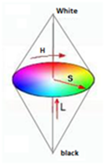
The HSL model comes from the work of painter Albert Munsell (1858-1918), and designed and introduced in the 1970s by computer graphics researchers in 1979 to align more closely with how human vision perceives color-making attributes. This color model contains three components: hue, saturation, and luminance. While saturation and luminance are “conventionally” encoded in scalar form, hue is an angular value. These components can be interpreted as follows:
Hue: represent the perceived color (red, yellow, green…). Hue is expressed by a number which is an angular position on the chromatic circle (starting from the top, clockwise). Example: red: 0°; green: 120°; magenta: 300°.
Saturation: measures the intensity or the purity of color, it is to say the percentage of pure color compared to the white. Saturation thus makes it possible to distinguish a bright color from a diluted color. Saturation is represented on the radius of the circle, by a percentage of purity: it is maximum on the circle 100% and minimal in the center (0=gray).
The luminance: define the part of black or white in the desired color (clear color or sinks).
The whole of the colors is represented inside a double cone (Figure 2). The luminance varies on the vertical axis of the double cone (axis of the gray) from the black in the bottom towards the white on top. The luminance is expressed by a percentage: from 0% (black) to 100% (white).
Based on these general concepts, various authors have proposed their own HSL model. Thus, we can cite the models described in the work of Travis [27] or Gonzalez and Woods [28] or the model introduced more recently by Serra [29]. For an extended panorama, the reader can refer to the researches [30, 31]. The great variability of the HSL models introduced necessarily implies different conversion formulas. We will use in this paper a recent model cited in the study [32].
Figure 2. HSL color space components
3.1.1 Conversion RGB to HSL
The passage from RGB to HSL color space is given by algorithm 1.
|
Algorithm 1 Conversion RGB to HSL |
$M=\max \left\{ R,G,B \right\}$ $m=\min \left\{ R,G,B \right\}$ $if\ M=m\to H=0$ $if\,M\ne m,$ $if\,M\equiv R,\quad H=0+\frac{G-B}{M-m}$ $if\,M\equiv G,\quad H=2+\frac{B-R}{M-m}$ $if\,M\equiv B,\quad H=4+\frac{R-G}{M-m}$ $H=H\times 60$ $if\ H<0\to H=H+360$
$L=\frac{M+m}{2}$
$\begin{align} & if\ L\le 0.5 \\ & S=\frac{M-m}{2\times L} \\ & f\ L>0.5 \\ & S=\frac{M-m}{2-2\times L} \\\end{align}$ Remark1 M and m are intermediation variables. |
3.1.2 Robustness to illumination condition changes
The HSL model provides additional information through its three components. It has the advantage of allowing the development of robust methods to changes in lighting. Indeed, these artefacts mainly affect the luminance component. By taking into account only the chrominance components (hue and saturation), it is thus possible to reduce the sensitivity to changes in illumination [33]. We also observed that hue was a more robust component than saturation or luminance in a multi-resolution setting. The hue is therefore an interesting invariant component with changes in lighting and multi-resolutions of the executive. However, it should be analyzed with caution. Indeed, its reliability depends on the saturation level and the color is significant only if the saturation is high. Hue-based analysis methods must therefore check for pixels that are not achromatic [33].
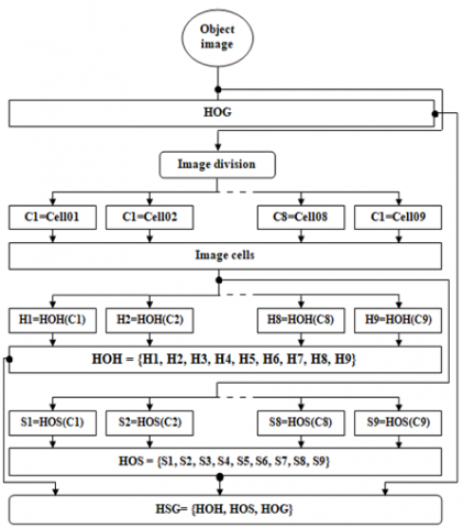
3.2 HSG (Hue, Saturation, Gradient) descriptor
To reach our combined HSG descriptor (Figure 3), the first step is to calculate the Oriented Gradient Histogram (HOG), after which we move to create the image cells to build the Oriented Hue Histogram (HOH) and the oriented saturation histogram (HOS). The last step is to assemble the three descriptors into a characterization descriptor called the HSG descriptor. While the HOG building steps were detailed in section 2.1, here we only explain the HOH and HOS building steps.
Figure 3. HSG descriptor Building steps
3.2.1 Histogram of oriented gradient
To build our HOG, we take 9 as the number of bins and 3 as the number of HOG windows per linked box, so our HOG will be a vector composed of 81 values.
3.2.2 Image cells
Figure 4. Image division result (descriptor cells)
Blocks (cells) and bin ideas is an efficient method to give the description the necessary stability in the face of variations in geometric conditions [34]. To this end, the first step of our proposed descriptor is to divide the object image into connected areas overlapped at 50% called cells (Figure 4). Ditto for the HOG, we chose the number 9 for the number of cells and bins.
3.2.3 Histogram of oriented hue
To construct the oriented hue histogram for cell 01, first the hue angle range (360 degrees) is divided into 9 parts (bins) each bin will represent 40 degrees:
$Hue=\left[ \begin{align} & bin1\cup bin2\cup bin3\cup bin4\cup bin5 \\ & \cup bin6\cup bin7\cup bin8\cup bin9 \\\end{align} \right]$ (10)
With:
$\begin{align} & bin01=\left[ {{000}^{o}},{{039}^{o}} \right],bin02=\left[ {{040}^{o}},{{079}^{o}} \right], \\ & bin03=\left[ {{080}^{o}},{{119}^{o}} \right],bin04=\left[ {{120}^{o}},{{159}^{o}} \right], \\ & bin05=\left[ {{160}^{o}},{{199}^{o}} \right],bin06=\left[ {{200}^{o}},{{239}^{o}} \right], \\ & bin07=\left[ {{240}^{o}},{{279}^{o}} \right],bin08=\left[ {{280}^{o}},{{319}^{o}} \right], \\ & bin09=\left[ {{320}^{o}},{{359}^{o}} \right], \\\end{align}$
Now the hue value of each pixel in cell 01 is calculated and then added to the magnitude of its corresponding bin. Towards the end, we get a descriptor vector of value 12, each value corresponds to the magnitude of a bin (M.bin).
$\text{Descriptor =}\left[ \begin{align} & \text{M}\text{.bin}01,\text{M}\text{.bin}02,\text{M}\text{.bin}03,\text{M}\text{.bin}04, \\ & \text{M}\text{.bin}05,\text{M}\text{.bin}06,\text{M}\text{.bin}07,\text{M}\text{.bin}08, \\ & \text{M}\text{.bin}09,\text{M}\text{.bin10,M}\text{.bin11,M}\text{.bin12} \\\end{align} \right]$ (11)
To get the final cell01 descriptor (D cell 01), we normalize this vector (Eq. (10)) with the L2 normalization (Eq. (1)).
$\text{D cell 01 =}\left[ \begin{align} & \text{M }\!\!'\!\!\text{ }\text{.bin}01,\text{M }\!\!'\!\!\text{ }\text{.bin}02,\text{M }\!\!'\!\!\text{ }\text{.bin}03,\text{M }\!\!'\!\!\text{ }\text{.bin}04, \\ & \text{M }\!\!'\!\!\text{ }\text{.bin}05,\text{M }\!\!'\!\!\text{ }\text{.bin}06,\text{M }\!\!'\!\!\text{ }\text{.bin}07,\text{M }\!\!'\!\!\text{ }\text{.bin}08, \\ & \text{M }\!\!'\!\!\text{ }\text{.bin}09,\text{M }\!\!'\!\!\text{ }\text{.bin10,M }\!\!'\!\!\text{ }\text{.bin11,M }\!\!'\!\!\text{ }\text{.bin12} \\\end{align} \right]$ (12)
With:
M'.bin is the normalized value of M'.bin.
By repeating this method for the other eight cells, we end up with nine cell characterization vectors, each vector contains nine values, and each value corresponds to the magnitude of a bin. Once we group the nine cell characterization vectors, we obtain the final oriented histogram of the hue (composed of 81 values).
$\text{ HOH=}\left[ \begin{align} & \text{D cell 01},\text{D cell 02},\text{D cell 03},\text{D cell 04}, \\ & \text{D cell 05},\text{D cell 06},\text{D cell 07},\text{D cell 08}, \\ & \text{D cell 09},\text{D cell 10,D cell 11,D cell 12} \\\end{align} \right]$ (13)
3.2.4 Histogram of oriented saturation
The same steps of the oriented hue histogram are repeated, but this time we use the saturation values instead of the hue values.
3.2.5 HSG descriptor
Finally, and by assembling the three final vectors (HOH, HOS and HOG) into a single vector, we obtain the final HSG descriptor (Figure 3). This descriptor is a vector composed of 243 values (81 * 3).
In this section, we present the different classification methods used and implemented within the framework of this article, the K-Nearest Neighbor (KNN) and the Support Vector Machine (SVM).
4.1 KNN (K-Nearest Neighbor)
The k-nearest neighbor algorithm is a nonparametric method proposed by Altman [35] used for regression and classification. KNN is based on a direct comparison between the characteristic vector of the instance to be classified and the vectors of the instances of the learning base. When a new input arrives, it is compared to the learning materials using a similarity measure by calculating the distances between these instances. In a classification problem, we will retain the most represented class among the k outputs associated with the k inputs closest to the new input x. There are several distances used by the KNN algorithm to compare two instances.
Let $X_{i}=\left(x_{i} 1, x_{i} 2, \ldots, x_{i} n\right)$ denote the characteristic vector of instance is, with n the number of variables and by p and q two instances to compare. The principal distances used by the KNN algorithm to compare two instances are:
Euclidean distance: the Euclidean distance is given by:
$D\left( {{X}_{P}},{{X}_{q}} \right)=\sqrt{\sum\limits_{i=1}^{n}{{{\left( {{x}_{P}}i-{{x}_{q}}i \right)}^{2}}}}$ (14)
Manhattan distance: the Manhattan distance is given by:
$D\left( {{X}_{P}},{{X}_{q}} \right)=\sum\nolimits_{i=1}^{n}{\left| \left( {{x}_{P}}i-{{x}_{q}}i \right) \right|}$ (15)
Minkowski distance: the Minkowski distance is given by:
$D\left( {{X}_{P}},{{X}_{q}} \right)={{\sum\nolimits_{i=1}^{n}{\left( {{\left( {{x}_{P}}i-{{x}_{q}}i \right)}^{r}} \right)}}^{\frac{1}{r}}}$ (16)
Tchebychev distance: the Tchebychev distance is given by:
$D\left( {{X}_{P}},{{X}_{q}} \right)=\max _{i=1}^{n}\left| {{x}_{P}}i-{{x}_{q}}i \right|$ (17)
4.1.1 Choice of “k”
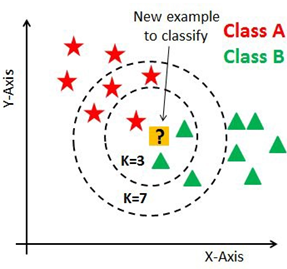
The value of k is one of the parameters to be determined when using this type of method. The value that we choose k will be more critical, more determining in relation to the performance of the classifier (Figure 5).
There are no predefined statistical methods to find the most favorable value of K. However, some researchers e.g. [36, 37], found that k = 1 is the optimal value when performing a categorization task, because when k = 1, the KNN algorithm classifies the object to its nearest neighbor. In this article, and after many tests, we found that k = 1 gives the best recognition rate, so we decided to use this value in all our experiments.
Figure 5. The choice of "k" influences the decision: as you can verify from the image above, if we proceed with K = 3, then we predict that the test entry belongs to class B, and if we continue with K = 7, then we predict this test entry belongs to class A
4.2 SVM (Support Vector Machine)
SVM is a very popular supervised binary classification technique [38] which was developed in the 1990s from theoretical considerations of Vladimir Vapnik. It is based on maximizing the classifier margin, i.e., the distance between the decision boundaries and the closest samples. These boundaries are called support vectors. For a binary classification, the decision function of SVM is defined by:
$g\left( x \right)=\sum\limits_{i}{{{\omega }_{i}}}{{y}_{i}}k\left( {{x}_{i}},z \right)-b$ (18)
where, w is the vector orthogonal to the hyper-plane, k(xi,z) is the function used for training data xi and a test z. yi is the label of the class of xi and b is the threshold. In general, depending on the value of k(xi,z), there are two types of SVM: linear and non-linear.
4.2.1 Linear SVM
This method is considered to be the simplest classifier to calculate. It consists in finding a hyperplane which separates the two classes obtained by a linear combination of characteristics. Consider a learning set $\left\{\left(z_{i}, y_{i}\right)\right\}_{i=1}^{n}, y_{i} \in y \in$ $\{1, \ldots, L\}$, a linear SVM consists of learning linear functions $L\left\{\omega_{c}^{T} z \mid c \in y\right\}$, knowing that for a test set $\mathrm{z}$, the value of $k(x, z)$ is:
$k\left( {{x}_{i}},z \right)=z$ (19)
4.2.2 Nonlinear SVMs
This classifier shows excellent results in the task of categorizing images. It uses nonlinear kernels to classify data that is not linearly separable. The idea here is to project the data onto a new, very large representation space where the data is linearly separable. The most used nonlinear kernels (K [xi, z]) are kernels with Mercer properties, e.g. intersection of kernels [39], chi-square kernels [40], Gaussian kernels, polynomials, RBF.
In the case of a multi-class classification, we generally apply the one-against-all strategy where a linear function L is computed by solving a convex optimization problem [41]:
${{\min }_{{{\omega }_{c}}}}\left\{ J\left( {{\omega }_{i}} \right)={{\left\| {{\omega }_{i}} \right\|}^{2}}+c\sum\limits_{i=1}^{n}{l\left( {{\omega }_{i}};y_{i}^{c},zi \right)} \right\}$
where ${{y}_{i}}=\left\{ \begin{align} & 1\quad if\,{{y}_{i}}=c \\ & -1\quad else \\\end{align} \right.$
and $l\left( {{\omega }_{i}};y_{i}^{c},zi \right)={{\left[ \max \left( 0,\omega _{c}^{T}\,z.y_{i}^{c}-1 \right) \right]}^{2}}$ (20)
In this paper experiments, we will use the polynomial Kernel function of Matlab 2018b with an automatic Kernel scale. To use the SVM source code used in this article, the reader may refer to [42].
In this section we begin by presenting the database and justifying the choices of these in our experiments, then we move on to designate the evaluation criteria. Finally comes the presentation and discussion of the results.
5.1 Image database
We tested our approach to categorize color objects using two publicly available datasets, the Columbia Object Image Library (COIL-100) [43], and The Amsterdam Library of Object Images (ALOI) [44].
5.1.1 Columbia object image library (COIL-100)
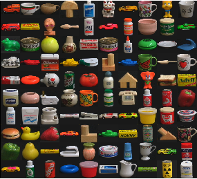
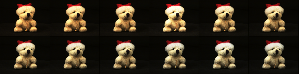
This dataset contains a set of color images (128×128 pixels) of 100 objects with 72 different views for each object (Figure 6) at different angles of rotation. Images were taken at 5 degree exposure intervals (Figure 7). This variation in angles and pose make the COIL-100 dataset ideal for testing invariance to changes in geometric conditions. In our experience, 22 images will be used for the training set and 50 images for the test set.
Figure 6. Samples of images from the coil-100 database
Figure 7. An object from the coil-100 database with different orientations and scale changes
5.1.2 The Amsterdam Library of object images (ALOI)
This dataset contains a total of 110,250 images of 1,000 different objects (Figure 8), in this article we use the version (384 x 288 pixels) of the images. In short, we can classify these dataset images into 3 subsets, ALOI-Viewpoint, ALOI-illumination angle and ALOI-illumination color:
Figure 8. Samples of images from Amsterdam Library of Object Images
-ALOI-Viewpoint: in this part, the images were photographed in rotation. Each photo is taken after the object has been rotated 5 degrees, resulting in 72 photos for each object (Figure 9).
Figure 9. Example objects from ALOI viewed under different angles
-ALOI-illumination angle: the images were taken in 24 different illumination directions, resulting in 24 photos for each object (Figure 10).
-ALOI-illumination color: the images were taken under 12 different illumination color temperatures, resulting in 12 photos for each object (Figure 11).
Figure 10. Example objects from ALOI viewed under 24 different illumination directions [45]
Figure 11. Example objects from ALOI-COL viewed under 12 different illumination color temperatures
Similar to COIL-100, the ALOI-Viewpoint dataset is widely used in experiments that study invariance to changes in geometric conditions. While the large variation in lighting conditions in ALOI-illumination angle and ALOI-illumination color makes this database optimal for testing invariance to changing illumination conditions. In our experiment, we collect the ALOI-illumination angle and ALOI-illumination color together in a group (ALOI-illumination), which has 36 photos for each object. 11 images will be used for the training set and 25 images for the test set. For ALOI-Viewpoint, and even for COIL-100, 22 images will be used for the training set and 50 images for the test set.
5.2 Evaluations criteria
F-measure is the summary indicator commonly used for 25 years to evaluate the algorithms of data classification, based on precision and recall. In this paper, we use a criterion similar to the one proposed by Ke and Sukthankar [46] and Goutte and Gaussier [47].
5.2.1 Precision
The precision (P), or positive predictive value, is the proportion of recognized items among all the items offered.
$\mathrm{P}=\frac{\text { Recognized images }}{\text { Recognized images }+\text { Unrecognized images }\quad}$ (21)
In statistics, precision is called the positive predictive value.
5.2.2 Recognition rate
The Recognition rate can be calculated using the precision criterion cited in Eq. (21):
Recognition rate $(\%)=\mathrm{P} * 100$ (22)
5.2.3 Response time
In technology, response time is a measure of the performance of an interactive application. It can be defined as the time lag between an electronic input and the output signal. In our system, we define the response time as the time elapsed between the start of the request and the end of categorization.
All those 3 evaluation criteria will be used to evaluate the performance of our proposed descriptor.
5.3 Parametric tests
In this part, we aim to do a test on our proposed descriptor parameters, including: combination organization, training database size and test database size.
5.3.1 Test configuration
Each test in this section contains 3 parts: test on COIL-100 datasets, tests on AlOI-view datasets and tests on AlOI-illumination datasets and for the 3 parts we will do one test on 50 objects. As mentioned before, for the first and second parts of the test (COIL-100 and AlOI-view tests), each object is represented with 72 images, 22 images will be used in the training set and 50 images in the set of tests.
For all the tests in this part, we use the SVM classifier and the KNN classifier, our first priority is to find the combination that gives the highest recognition rate, then if we find multiples, we take the combination that has the highest recognition rate and shortest response time.
5.3.2 Combination location tests
We propose in this article the use of three descriptors: the famous descriptor HOG (We symbolize it in this test by G), the new descriptor HOH proposed (We symbolize it by H) and the new descriptor HOS proposed (We symbolize it by S). The goal of this test is to find the combination of these three descriptors which give the highest recognition rate. For that we will try in this part of the test all the possible combinations which are:
—Singular descriptors (H, G and S), so each descriptor will be tested separately.
—Two by two descriptors, by changing the location of the singular descriptors in the combination, which are: GH (this means that the 81 values of the descriptor G are placed first followed by the 81 value of the descriptor H), GS, HG, HS, SG and SH.
—Three by three descriptors, changing the location of the singular descriptor in the combination, which are: GHS (this means that the 81 values of the G descriptor are placed first, the 81 values of the H descriptor are placed second and the 81 values of the descriptor S are placed in the last position), GSH, HGS, HSG, SGH and SHG.
Figure 12 shows the result of applying these descriptors on the coil-100 database, while Figure 13 and Figure 14 show the result of applying on the ALOI database.
Figure 12. Combination location tests on COIL-100 dataset
Figure 13. Combination location tests on ALOI-view dataset
Figure 14. Combination location tests on ALOI-illumination dataset
As shown in Figure 12, Figure 13 and Figure 14, three-by-three combinations have the highest recognition rate. We also noticed that the location of the descriptor in the combinations has no influence on the recognition rate, because all three-by-three combinations have the same recognition rate on the same data set. Same for double combinations which have the same component (e.g., GH and HG) also have the same recognition rate on the same data set.
Because the recognition rate of the trilogy combinations is the same, we will use the response time of the trilogy descriptors to designate the best combination.
Testing was performed using Matlab 2018b 64 bits in a Toshiba P50 laptop with i7-4700MQ 2.40GZH CPU, 8 GB RAM and dual graphics card, Intel 4400 hd and NVIDIA GeForce GT 745M. The time reported in Table 1 is the time that was consumed to complete the categorization of 2,500 images for the COIL-100 tests and the ALOI-view test, and 1,250 images for the ALOI-illumination.
From the results presented in Table 1, we notice that the HSG combination has the lowest categorization time in 4 tests versus one for each of the HGS and SHG combinations. We therefore recommend that you use this HSG combination, and we will use this combination in the rest of our article.
We also note the great speed of KNN classifiers compared to SVM classifiers, you will find a detailed comparison between these two classifiers in the rest of the article.
Table 1. Categorization time of trilogy combinations descriptors
|
|
COIL-100 |
ALOI-view |
AlOI-ill |
|||
|
SVM |
KNN |
SVM |
KNN |
SVM |
KNN |
|
|
GHS |
1431 |
69 |
1835 |
398 |
988 |
197 |
|
GSH |
1449 |
72 |
1781 |
397 |
1230 |
196 |
|
HGS |
1437 |
70 |
1771 |
396 |
887 |
198 |
|
HSG |
1430 |
68 |
1841 |
397 |
885 |
195 |
|
SGH |
1498 |
69 |
1773 |
395 |
888 |
196 |
|
SHG |
1441 |
69 |
1736 |
393 |
887 |
198 |
5.3.3 Training dataset size influence
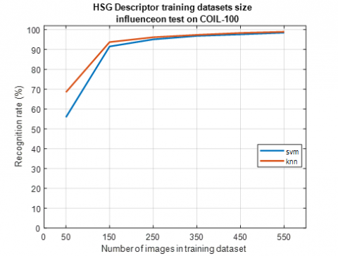
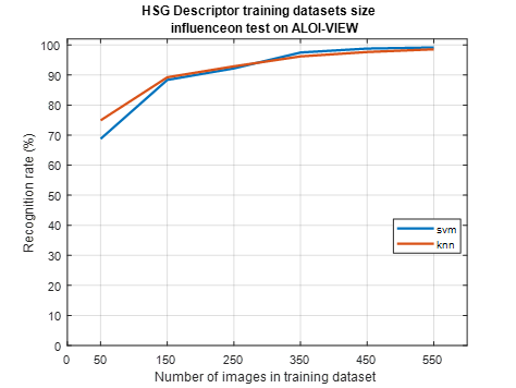
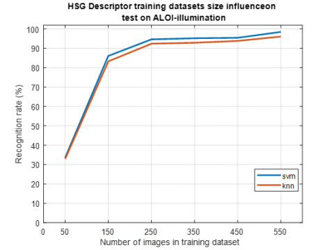
In previous tests, we found that HSG is the best combination of hue, saturation, and gradients. In this test, we focus on the influence of the training dataset on this HSG descriptor. To this end, we do a test on 50 objects, for each object we have 50 images of the test for COIL-100 and ALOI-view, and 25 images for ALOI-illuminance. The tests are carried out by varying the quantity of training images for each image, we take 1 training image for each object (therefore 50 images in the dataset), 3 images (therefore 150 images in the dataset), 5 images (therefore 250 images in the dataset), dataset), 7 images (therefore 350 images in the dataset), 9 images (therefore 450 images in the dataset) and finally 11 images (therefore 550 images in the dataset). Classification is performed using the KNN and SVM classifiers and the results are shown in Figure 15, Figure 16 and Figure 17.
Figure 15. HSG Descriptor training datasets size influence on COIL-100 dataset
The amount of data for training and test validation remains an open issue. However, most researchers have a good experience with 50% data for training and 50% for testing, but 50% for training data requires a lot of storage resources. Figure 15, Figure 16 and Figure 17 show that there is a positive correlation relationship between the size of the training data set and the recognition rate of HSG descriptors, it means that the increase in the Training dataset size can improve the recognition rate of the proposed descriptor. Otherwise, this increase may slow down the categorization task, and also increase the required storage and memory size. That's why we need to adjust the size of the training dataset to balance the recognition rate and the other parameters we just mentioned.
Figure 16. HSG descriptor training datasets size influence on ALOI-view dataset
Figure 17. HSG descriptor training datasets size influence on ALOI-illumination dataset
To achieve this balance, we recommended using 30-35% in the training dataset. This 30 to 70% is located halfway between the cross validation of the iv and v folds. In fact, when cross-validating, we can choose one of the LOOCV, v-fold, x-fold methods. Very often the V-fold gives the best results. So just maintaining 30% for training is a simplified version of v-fold [48, 49].
5.3.4 Test dataset size influence
The aim of this test is to study the influence of the size of the datasets on the recognition rate of HSG descriptors. For this we carry out tests by varying the number of objects to be tested. We use 10 items, 20 items, 30 items, 40 items and 50 items. Each object is represented with 50 tests image for COIL-100 and AlOI-view, while for ALOI-illumination we use 25 images in tests. For training data sets 22 images are used in the training set of COIL-100 and AlOI-view with 11 images for ALOI-illumination. For tests with 10 objects the total of the test images is 500, for the tests with 20 objects the total of the test images is 1000, for the tests with 30 objects the total of the test images is 1500, for tests with 40 objects the total of the test images is 2000 and for the test with 50 objects the total of the test images is 2500. Results are shown in Figure 18, Figure 19 and Figure 20.
Figure 18. HSG descriptor test datasets size influence on COIL-100
Figure 19. HSG descriptors test datasets size influence on ALOI-view
Figure 20. HSG descriptor test datasets size influence on ALOI-illumination
Unlike the previous test, Figure 18, Figure 19 and Figure 20 show that there is a negative correlation relationship between the size of the test data sets and the recognition rate of the HSG descriptors. This means that increasing the size of the data set may decrease the recognition rate of the proposed descriptor. This decrease is due to the entry of new objects that may be similar to objects that already exist in the datasets. This is why we have proposed in this article to combine the colors of the objects with its outlines (contours). This combination can make the proposed descriptor better able to distinguish similar objects. Despite this, in our opinion, this decrease is not significant when compared to the rapid increase in tested objects, and the results of the HGS descriptor are largely satisfactory when compared with other old and existing methods. In the rest of the article, readers can find a detailed comparison of the results of the proposed descriptors with the results of the existing categorization methods.
5.4 Comparative tests
In this part, we aim to make a comparative study between the proposed HSG descriptor and other existing methods: HOG descriptors, hue histograms, opponent histograms, the local image descriptor from even Gabor filter response descriptors and the hue descriptors. We first focus on the recognition rate of each method, and then we move on to comparing the response time of those methods.
5.4.1 Stability test against changes in geometric conditions
This part of the tests is performed on 50 objects from the COIL-100 datasets and 50 objects from ALOI-view date set. Each object is represented with 22 images in the training set and 50 images in the tests. Each image will be encoded using HOG descriptors (HOG) [15], opponent histograms (OPP) [22], hue histograms (Hue H) [21], Gabor descriptors (Gabor) [26], the hue descriptor (Hue D) [21] and the proposed combining HSG descriptor.
For HOG settings, 9 is considered the number of boxes and 3 is the number of windows per linked box. The opponent's histograms and the hue histograms quantified at 36 bins, 2 are the smooth flags and lambda = 1. For the hue descriptors, 25 corresponds to the number of cells and 12 to the number of bins. For the proposed HSG descriptor, we use the same HOG parameters cited with 9 cells and 9 bins for HOH and HOS. In this part of the test, we focus on the methods recognition rate and the average time to classify an object. The latter is calculated by dividing the total sum of the method tests by the total number of images tested (2,500 images in this part of the test). The software and hardware environment is the same as above.
Table 2. Test of stability against geometric conditions changes on COIL-100 using SVM
|
|
R.Rate [%] |
T.T [S] |
A.T[S] |
|
HOG [15] |
84.04 |
988 |
0.39 |
|
OPP [22] |
87.28 |
4947 |
1.98 |
|
Hui H [22] |
89.28 |
4949 |
1.98 |
|
Hui D [21] |
95.12 |
2576 |
1.03 |
|
HSG |
98.44 |
1430 |
0.57 |
Table 3. Test of stability against geometric conditions changes on ALOI-view using SVM
|
|
R.Rate (%) |
T.T (s) |
M.T |
|
HOG [15] |
85.36 |
1175 |
0.47 |
|
OPP [22] |
79.40 |
11792 |
4.71 |
|
Hui H [22] |
80.12 |
20074 |
8.02 |
|
GABOR [26] |
74.36 |
75405 |
30.02 |
|
Hui D [21] |
96.20 |
2103 |
0.84 |
|
HSG |
99.16 |
1841 |
0.73 |
Table 4. Test of stability against geometric conditions changes on COIL-100 using KNN
|
|
R.Rate [%] |
T.T [S] |
A.T[S] |
|
HOG [15] |
81.76 |
42 |
0.02 |
|
OPP [22] |
87.04 |
309 |
0.12 |
|
Hui H [22] |
92.48 |
133 |
0.05 |
|
Hui D [21] |
95.68 |
92 |
0.04 |
|
HSG |
98.92 |
68 |
0.03 |
Table 5. Test of stability against geometric conditions changes on ALOI-view using KNN
|
|
R.Rate (%) |
T.T (s) |
M.T |
|
HOG [15] |
85.08 |
266 |
0.11 |
|
OPP [22] |
84.96 |
99 |
0.04 |
|
Hui H [22] |
84.96 |
105 |
0.04 |
|
GABOR [26] |
86.76 |
970 |
0.38 |
|
Hui D [21] |
96.96 |
399 |
0.16 |
|
HSG |
98.56 |
397 |
0.16 |
The classifiers are trained to use all but one of the images. The image used in the training set is not used in the test. Tables 2 and 3 show the recognition rate percentage (R.rate [%]), the total test time per second (TT [S]) and the average time per second (AT [S]) using the classifiers SVM. While Table 4 and Table 5 show the same results using KNN classifiers.
From the results presented in the last four tables, the proposed HSG has the best recognition rate in all experiments, 98.44% on COIL-100 using SVM, 99.16% on ALOI-view using SVM, 98.92% on COIL-100 using KNN and 98.56% on ALOI-view using KNN.
The superiority of colors in the task of recognizing and categorizing objects was confirmed by these tests. We see that in all the tests, the results of the descriptor using colors (hue histogram [22], opponent histograms [22] and the hue descriptor [21]) are better than the other descriptors.
The effectiveness of the cell-and-pan method against changing geometric conditions was also confirmed by these tests. It is easy to notice that the hue descriptor and the HSG descriptor have a higher recognition rate than the other method in all the tests. While in the HOG results, this cell and bin method was not sufficient to obtain good results, due to the use of the gradient which was not sufficient to allow the descriptor to have a good distinction between objects (for example, Figure 1).
From the results of the COIL-100 tests (Table 2 and Table 4), it can be seen that the gradient-color combination proposed in the HSG descriptors, improved the HOG recognition rate by 14% in SVM classifiers tests and 17% in KNN classifiers tests. But the response time increased from 0.39 seconds to 0.57 seconds in SVM classifier tests, and from 0.02 seconds to 0.03 seconds in KNN classifier tests. This increase in response time is due to the fact that the calculation of the HOG descriptor is part of the calculation of the HSG descriptor, so it is normal.
Same thing in the results of the ALOI-view tests (Table 3 and Table 5), the recognition rate of HSG descriptors improved by approximately 14% in the SVM classifier tests and by 13% in the KNN classifier tests. While the response time increased from 0.47 seconds to 0.73 seconds in SVM classifier tests, and from 0.11 seconds to 0.16 seconds in KNN classifier tests.
From the result of the opponent and hue histograms, as well as the result of Gabor on the datasets of the ALOI view, we can conclude that these descriptors do not have sufficient stability against changes in geometric conditions. By using the cells a bins idea, we were able to enhance the stability of our proposed HSG descriptor, which is why there is a great improvement in our HSG descriptor recognition rate against these descriptors in all tests. We also note the very high categorization time of these descriptors compared to the proposed HSG categorization time, which demonstrates the difficulties of categorization tasks using these descriptors in the presence of changes in geometric conditions. We remind you that we did not do a Gabor descriptor test on COIL-100, because this descriptor does not support the COIL-100 image size (128×128 pixels).
Compared to the results of the hue descriptor, the combination of the gradient with colors improved the ability of the HSG descriptor to distinguish objects having similar colors. This improvement can easily be seen from the recognition rates, in the COIL-100 test, the recognition rates went from 95.12% to 98.44% using the SVM classifiers, and from 95.68% to 98.92% using KNN classifiers. In the ALOI-view test, it went from 96.20% to 99.16% using SVM classifiers, and from 96.96% to 98.56% using KNN classifiers.
For categorization time, the HSG is faster than the hue descriptor in the coil 100 test, its average categorization time of 0.57 seconds using SVM classifiers and 0.03 seconds using KNN classifiers, while for the hue descriptor, the average categorization time is 1.03 seconds using SVM classifiers and 0.04 seconds using KNN classifiers.
In the ALOI-view test, the HSG is also faster with an average categorization time of 0.73 seconds using the SVM classifiers and 0.16 seconds using the KNN classifiers, while for the hued descriptor, the time average categorization time is 0.84 seconds using SVM classifiers and 0.16 seconds using KNN classifiers. This improvement in response time is due to the small size of the HSG descriptor (243 values) compared to the size of the hue descriptor (300 values). The limited size of the HSG descriptor also optimizes the use of memory space, the difference in performance is then clearly indicated.
In the COIL-100 dataset test, KNN classifiers have a better recognition rate than SVM for categorization tasks with the HSG descriptor. Whereas, in testing ALOI-view datasets, the recognition rate using SVMs is better. For categorization time, KNN classifiers performed remarkably better than SVM classifiers in all tests.
5.4.2 Stability test against changing illumination conditions
This part of the tests is done on the 50 same objects used in the ALOI-view test, but this time we use the ALOI-illumination part. Each object is represented with 11 images in the training set and 25 images in the tests. Each image will be encoded using HOG descriptors (HOG) [15], opponent histograms (OPP) [22], hue histograms (Hue H) [22], Gabor descriptors (Gabor) [26], the hue descriptor (Hue D) [21] and the proposed combining HSG descriptor. The descriptor parameters are the same as those of the previous part of the test.
Also in this part of the test, we focus on the method recognition rate and the average time to categorize an object. The latter is calculated by dividing the total time of tests of the methods over the total number of images tested (1250 images in this part of the test). The software and hardware environment is the same as mentioned above.
Table 6. Test of stability against photometric conditions changes on ALOI- illumination using SVM
|
|
R.Rate (%) |
T.T (s) |
M.T |
|
HOG [15] |
81.84 |
341 |
0.27 |
|
OPP [22] |
88.48 |
1913 |
1.37 |
|
Hui H [22] |
91.76 |
910 |
0.73 |
|
GABOR [26] |
91,92 |
2084 |
1.67 |
|
Hui D [21] |
96.40 |
907 |
0.73 |
|
HSG |
98.48 |
885 |
0.68 |
Table 7. Test of stability against photometric conditions changes on ALOI- illumination using KNN
|
|
R.Rate (%) |
T.T (s) |
M.T |
|
HOG [15] |
82.64 |
134 |
0.11 |
|
OPP [22] |
89.04 |
445 |
0.36 |
|
Hui H [22] |
93.52 |
231 |
0.18 |
|
GABOR [26] |
91.76 |
414 |
0.33 |
|
Hui D [21] |
93.76 |
238 |
0.19 |
|
HSG |
96.08 |
195 |
0.16 |
The classifiers are trained to use all but one image, which is used in the test. Table 6 shows the percent recognition rate (R.rate [%]), total test time per second (T.T [S]), and the average time per second (A.T [S]) using the SVM classifiers. While Table 7 shows these results using KNN classifiers.
The results presented in Table 6 and Table 7 prove that the proposed HSG descriptor has better performance than all other methods. It has a recognition rate of 98.48% with SVM classifiers and 96.08% with KNN classifiers.
The theoretical property of hues has been proven by the results presented in Table 6 and Table 7, due to the stability of this chrominance component against changes in lighting conditions, the descriptors using hue values (the hue histogram, hue descriptor and HSG descriptor proposed in this paper) was more stable and obtained the highest recognition rates compared to other methods.
The combination of color-gradients allowed us to solve the problem of missing stability against the shadows and lighting geometry changes such as shading, the illumination color and light scattering, the highlights under a white light source and the scattering of a white light source, and the problem of objects with similar edge. By solving all these problems in the proposed HSG descriptor, we were able to increase the recognition rate from 81.84% to 98.48% using the SVM classifiers, and from 82.64% to 96.08% using the classifiers KNN.
Compared to the hue histogram [22] and the hue descriptor [21], the proposed HSG descriptor has a better recognition rate with a better categorization time using both the SVM and KNN classifiers, which confirms, again, its outstanding performance. This high performance is due to the combing of the gradient with colors which make the proposed HSG descriptor capable of distinguishing the object with high precision in real time and under different conditions.
We also note the better performance of the hue descriptor [21] compared to the hue histogram [22], even if the last two descriptors cited use hue values, but using the entire image in the hue descriptor [21] with cells and the bins method improved the recognition rate.
The results of the Gabor descriptor [26] are much better in this part of the test (Table 6 and Table 7) compared to the changes in geometric conditions (Table 3 and Table 5), which confirms that this descriptor is designed to cope with only changes in lighting conditions.
In this part of the test (Table 6 and Table 7), and as for ALOI-view tests, the recognition rate of the HSG descriptor using SVM classifiers is better than that of KNN classifiers, while KNN classifiers were faster in all tests. So, in conclusion, we recommend the use of SVM classifiers with the proposed HSG descriptor, if the first priority is the recognition rate with a precise classification, but if the user seeks a fast classification even if with less precision, the KNN classifier can handle the task.
In this article, a new model for recognizing and categorizing multicolored objects has been proposed. The proposed model is based on the combination of colors and gradients to detect as much information as possible from the image. For the gradient part, we chose to use the famous HOG descriptor due to its huge capacity of extracting the contours of objects with great precision. While, for the colors part, we proposed two new descriptors inspired from the HOG descriptor, with changing the arc tangent to the chrominance components, hue and saturation, of the HSL color space. The use of these chrominance, hue and saturation components made the proposed HSG descriptor stable against changes in photometric and lighting conditions (light intensity change, light intensity shift, light intensity change and shift and light color change). In addition, using the ideas of cells and bins, we were able to add the required stability against geometric changes to the proposed model. For the classification task, we proposed the use of two powerful and widely used classifiers, the SVM (Support Vector Machine) and KNN (k-nearest neighbors) classifiers. The proposed model was evaluated on two publicly available datasets, Columbia Object Image Library (COIL-100) and The Amsterdam Library of Object Images (ALOI). Tests have proven not only the exceptional performance of this proposed HSG descriptor over existing methods in terms of recognition rates, but also its speed and ability to optimize memory and storage usage. In our future work, we plan to use the proposed descriptor to detect and categorize other types of objects such as cars, dogs, cats, etc. We also plan to compete in order to replace the use of the barcode in the stores (shopping center, pharmacies, etc.) with an application based on the proposed HSG descriptor.
The authors would like to thank the anonymous reviewers for their valuable comments and suggestions which greatly improved the quality of the paper, the General Directorate for Scientific Research and Technological Development of the Algerian Republic in general, without missing also to thank the SET laboratory of Blida 01 University.
[1] Biernacki, C., Mohr, R. (1999). Indexation et appariement d'images par modèle de mélange gaussien des couleurs (Doctoral dissertation, INRIA). In 17e Colloque GRETSI, Vannes, France, 291-294.
[2] Swain, M.J., Ballard, D.H. (1991). Color indexing. International Journal of Computer Vision, 7(1): 11-32. https://doi.org/10.1007/BF00130487
[3] Van de Wouwer, G., Scheunders, P., Livens, S., Van Dyck, D. (1999). Wavelet correlation signatures for color texture characterization. Pattern Recognition, 32(3): 443-451. http://dx.doi.org/10.1016/S0031-3203 (98)00035-1
[4] Hauta-Kasari, M., Parkkinen, J., Jaaskelainen, T., Lenz, R. (1996). Generalized co-occurrence matrix for multispectral texture analysis. In Proceedings of 13th International Conference on Pattern Recognition, 2: 785-789. http://dx.doi.org/10.1109/ICPR.1996.546930
[5] Larabi, M.C., Richard, N., Fernandez, C., Macaire, L. (2001). ‘L’aide au diagnostic pour les cancers de peau basée sur une indexation par la couleur, la texture, la forme. In ICISP’ 2001, Agadir, Morroco, 1055-1062.
[6] Mehtre, B.M., Kankanhalli, M.S., Narasimhalu, A.D., Man, G.C. (1995). Color matching for image retrieval. Pattern Recognition Letters, 16(3): 325-331. http://dx.doi.org/10.1016/0167-8655 (94)00096-L
[7] Paschos, G. (1998). Chromatic correlation features for texture recognition. Pattern Recognition Letters, 19(8): 643-650. http://dx.doi.org/10.1016/S0167-8655(98)00038-5
[8] Paschos, G. (2000). Fast color texture recognition using chromaticity moments. Pattern Recognition Letters, 21(9): 837-841. http://dx.doi.org/10.1016/S0167-8655(00)00043-X
[9] Panjwani, D.K., Healey, G. (1995). Markov random field models for unsupervised segmentation of textured color images. IEEE Transactions on Pattern Analysis and Machine Intelligence, 17(10): 939-954. http://dx.doi.org/10.1109/34.464559
[10] Pass, G., Zabih, R., Miller, J. (1997). Comparing images using color coherence vectors. In Proceedings of the Fourth ACM International Conference on Multimedia, pp. 65-73. http://dx.doi.org/10.1145/244130.244148
[11] Huang, J., Kumar, S.R., Mitra, M., Zhu, W.J., Zabih, R. (1997). Image indexing using color correlograms. In Proceedings of IEEE Computer Society Conference on Computer Vision and Pattern Recognition, pp. 762-768. http://dx.doi.org/10.1109/CVPR.1997.609412
[12] Zhou, J., Gao, D., Zhang, D. (2007). Moving vehicle detection for automatic traffic monitoring. IEEE Transactions on Vehicular Technology, 56(1): 51-59. http://dx.doi.org/10.1109/TVT.2006.883735
[13] He, D.C., Wang, L. (2010). Simplified texture spectrum for texture analysis. Journal of Communication and Computer, 7(8): 44-53.
[14] Lowe, D.G. (2004). Distinctive image features from scale-invariant key points. International Journal of Computer Vision, 60: 91-110. https://doi.org/10.1023/B:VISI.0000029664.99615.94
[15] Dalal, N., Triggs, B. (2005). Histograms of oriented gradients for human detection. In IEEE 2005 CVPR’05 Computer Society Conference on Computer Vision and Pattern Recognition, San Diego, CA, USA, pp. 886-893. http://dx.doi.org/10.1109/CVPR.2005.177
[16] Dalal, N. (2006). Finding People in Images and Videos. Ph.D. The National Polytechnic Institute of Grenoble, France.
[17] Manjunath, B.S., Ohm, J.R., Vasudevan, V.V., Yamada, A. (2001). Color and texture descriptors. IEEE Transactions on Circuits and Systems for Video Technology, 11(6): 703-715. https://doi.org/10.1109/76.927424
[18] Maggio, E., Smeraldi, F., Cavallaro, A. (2005). Combining colour and orientation for adaptive particle filter-based tracking. In BMVC. http://dx.doi.org/10.5244/C.19.79
[19] Yan, X., Wu, X., Kakadiaris, I.A., Shah, S.K. (2012). To track or to detect an ensemble framework for optimal selection. In European Conference on Computer Vision, pp. 594-607. https://doi.org/10.1007/978-3-642-33715-4_43
[20] Possegger, H., Mauthner, T., Roth, P.M., Bischof, H. (2014). Occlusion geodesics for online multi-object tracking. In proceedings of the IEEE Conference on Computer Vision and Pattern Recognition, pp. 1306-1313. https://doi.org/10.1109/CVPR.2014.170
[21] Hamdini, R., Diffellah, N., Namane, A. (2019). Robust local descriptor for color object recognition. Traitement du Signal, 36(6): 471-482. http://dx.doi.org/10.18280/ts.360601
[22] Van de Sande, K.E., Gevers, T., Snoek, C.G. (2008). A comparison of color features for visual concept classification. In Proceedings of the 2008 International Conference on Content-Based Image and Video Retrieval, pp. 141-150. http://dx.doi.org/10.1145/1386352.1386376
[23] Van de Weijer, J., Schmid, C. (2006). Coloring local feature extraction. In 9th European Conference on Computer Vision, Graz, Austria, Part II, pp. 334-348. http://dx.doi.org/10.1007/11744047_26
[24] Van de Weijer, J., Gevers, T., Bagdanov, A. (2006). Boosting color saliency in image feature detection. IEEE Transactions on Pattern Analysis and Machine Intelligence, 28(1): 150-156. http://dx.doi.org/10.1109/TPAMI.2006.3
[25] Van de Sande, K., Gevers, T., Snoek, C. (2010). Evaluating color descriptors for object and scene recognition. IEEE Transactions on Pattern Analysis and Machine Intelligence, 32(9): 1582-1596. http://dx.doi.org/10.1109/TPAMI.2009.154
[26] Zambanini, S., Kampel, M. (2013). A local image descriptor robust to illumination changes. In Kämäräinen J.K, Koskela M. (Eds) Image Analysis. SCIA 2013. Lecture Notes in Computer Science, 7944. http://dx.doi.org/10.1007/978-3-642-38886-6_2
[27] Travis, D. (1991). Effective Color Displays: Theory and Practice. London: Academic Press.
[28] Gonzalez, R.C., Woods, R.E. (1992). Digital Image Processing. Boston, MA, USA, Addison-Wesley.
[29] Serra, J. (2005). Morphological segmentations of colour images. In Mathematical Morphology: 40 Years On. 151-176. http://dx.doi.org/10.1007/1-4020-3443-1_15
[30] Carron, T. (1995). Segmentations d’images couleur dans la basse Teinte-Luminance-Saturation: approchenumérique et symbolique. Ph.D, Savoie Mont Blanc University, Chambéry, France.
[31] Vandenbroucke, N. (2000). Segmentation d’imagescouleur par classification de pixels dans les espacesd’attributscolorimétriquesadaptés: Application à l’analysed’image. Lille University, France.
[32] Nishad, P.M. (2013). Various colour spaces and colour space conversion. Journal of Global Research in Computer Science, 4(1): 44-48.
[33] Lefèvre, S., Vincent, N. (2006). Apport de l’espaceTeinte-Saturation-Luminance pour la segmentation spatiale et temporelle. Traitement du Signal, 23(1): 59-77
[34] Ilas, M., Ilas, C. (2018). A new method of histogram computation for efficient implementation of the HOG algorithm. Computers, 7: 3-18. http://dx.doi.org/10.3390/computers7010018
[35] Altman, N.S. (1992). An introduction to kernel and nearest-neighbor nonparametric regression. The American Statistician, 46(3): 175-185. https://doi.org/10.1080/00031305.1992.10475879
[36] Alzouhbi, A. (2017). Plant classification using SVM and KNN classifiers. Ph.D. Near East University. Nicosia.
[37] Jasim, S.S., Al-Taei, A.A.M. (2018). A comparison between SVM and K-NN for classification of plant diseases. Diyala Journal for Pure Science, 14(2): 94-105. http://dx.doi.org/10.24237/djps.1402.383B
[38] Burges, C.J. (1998). A tutorial on support vector machines for pattern recognition. Data Mining and Knowledge Discovery, 2(2): 121-167. https://doi.org/10.1007/978-3-540-92910-9_15
[39] Maji, S., Berg, A.C. (2009). Max-margin additive classifiers for detection. In 2009 IEEE 12th International Conference on Computer Vision, pp. 40-47. http://dx.doi.org/10.1109/ICCV.2009.5459203
[40] Zhang, J., Marszałek, M., Lazebnik, S., Schmid, C. (2007). Local features and kernels for classification of texture and object categories: A comprehensive study. International Journal of Computer Vision, 73(2): 213-238. http://dx.doi.org/10.1007/s11263-006-9794-4
[41] Yang, J., Yu, K., Gong, Y., Huang, T. (2009). Linear spatial pyramid matching using sparse coding for image classification. In 2009 IEEE Conference on Computer Vision and Pattern Recognition, pp. 1794-1801. http://dx.doi.org/10.1109/CVPR.2009.5206757
[42] Mishra, A. (2021). Multi Class Support Vector Machine (https://www.mathworks.com/matlabcentral/fileexchange/33170-multi-class-support-vector-machine), MATLAB Central File Exchange.
[43] Nene, S.A., Nayar, S.K., Murase, H. (1996). Columbia Object Image Library (COIL-100), Technical Report CUCS -006-96, Columbia Univ.
[44] Geusebroek, J.M.; Burghouts, G., Smeulders, A. (2005). The Amsterdam Library of object images. International Journal of Computer Vision, 61: 103-112. http://dx.doi.org/10.1023/B:VISI.0000042993.50813.60
[45] Hamdini, R. (2021). Reconnaissance d'objets par l'histogramme de couleurs orientées. Ph.D, Blida01 University, Blida, Algeria. http://dx.doi.org/10.13140/RG.2.2.22552.72966
[46] Ke, Y., Sukthankar, R. (2004). PCA-SIFT: A more distinctive representation for local image descriptors. In Proceedings of the 2004 IEEE Computer Society Conference on Computer Vision and Pattern Recognition, 2004. CVPR 2004, pp. II-II. http://dx.doi.org/10.1109/CVPR.2004.1315206
[47] Goutte, C., Gaussier, E. (2005). A probabilistic interpretation of precision, recall and F-score, with implication for evaluation. In European Conference on Information Retrieval, pp. 345-359. http://dx.doi.org/10.1007/978-3-540-31865-1_25
[48] Stone, M. (1974). Cross-validatory choice and assessment of statistical predictions. Journal of the Royal Statistical Society: Series B (Methodological), 36(2): 111-133.
[49] Larlus, D. (2008). Création et utilisation de vocabulaires visuels pour la catégorisation d'images et la segmentation de classes d'objets. Ph.D. The National Polytechnic Institute of Grenoble, France.