Swaraja Kuraparthi* | Madhavi K. Reddy | C.N. Sujatha | Himabindu Valiveti | Chaitanya Duggineni | Meenakshi Kollati | Padmavathi Kora | V. Sravan
© 2021 IIETA. This article is published by IIETA and is licensed under the CC BY 4.0 license (http://creativecommons.org/licenses/by/4.0/).
OPEN ACCESS
Manual tumor diagnosis from magnetic resonance images (MRIs) is a time-consuming procedure that may lead to human errors and may lead to false detection and classification of the tumor type. Therefore, to automatize the complex medical processes, a deep learning framework is proposed for brain tumor classification to ease the task of doctors for medical diagnosis. Publicly available datasets such as Kaggle and Brats are used for the analysis of brain images. The proposed model is implemented on three pre-trained Deep Convolution Neural Network architectures (DCNN) such as AlexNet, VGG16, and ResNet50. These architectures are the transfer learning methods used to extract the features from the pre-trained DCNN architecture, and the extracted features are classified by using the Support Vector Machine (SVM) classifier. Data augmentation methods are applied on Magnetic Resonance images (MRI) to avoid the network from overfitting. The proposed methodology achieves an overall accuracy of 98.28% and 97.87% without data augmentation and 99.0% and 98.86% with data augmentation for Kaggle and Brat's datasets, respectively. The Area Under Curve (AUC) for Receiver Operator Characteristic (ROC) is 0.9978 and 0.9850 for the same datasets. The result shows that ResNet50 performs best in the classification of brain tumors when compared with the other two networks.
brain tumor, data augmentation, deep convolutional neural networks, magnetic resonance images, transfer learning, support vector machine
The development of unusual cells in the human brain is called a brain tumor. Researchers don't completely comprehend the reasons for the brain tumor, however some risk factors help in tracing the brain tumor stage. The Brain tumor is categorized into two types, primary and secondary brain tumor. The Primary brain tumor mainly originates from the brain or any part of the brain without infecting the other parts of the body. Malignant and benign are the most common types of tumors. The Secondary brain tumor does not directly originate in the brain, but the tumor gets spread from different parts of the body. Malignant tumors are mostly considered secondary type tumors. A benign tumor can be further classified into meningiomas and gliomas; these are regarded as low-grade tumors. A malignant tumor is a high-grade tumor, classified into glioblastoma and astrocytoma.
The imaging practices like Magnetic Resonance Imaging (MRI), Computed Tomography (CT), Positron Emission Tomography (PET) and Single Photon Emission Computer Tomography (SPECT) are essentially utilized in investigating the brain images. MRI and CT imaging techniques are the most widely used among these techniques due to their high-resolution image quality and widespread availability. Brain tumor detection commonly uses MRI imaging technique rather than CT imaging technique because it can examine pathological or other physiological alternations of living tissues. The standard type of brain tumor resulting in adults is Gliomas, which can be identified with the help of magnetic resonance (MR) images of different categories, such as T1-weighted (T1), T2-weighted contrast-enhanced (T1c), T2-weighted and fluid-attenuated inversion recovery (Flair). Early detection of tumor plays an essential role in the treatment process. The radiologist uses classification methods to categorize the MR image as normal or abnormal. If the resultant outcome is odd, then the type of tumor is detected for the other treatment process. Manual classification is an expensive and time-taking assignment. In addition, they can get different conclusions from various observers or dissimilar findings from the similar observer in distinguishing tumor. Therefore, automatic classification techniques are obligatory.
Instead of developing a new model, deep transfer learning adapts an existing deep model that has already proven its effectiveness. As a result, the costs of complex layer parameters as well as prolonged validation processes are reduced.
The significant contributions of the proposed framework are listed as below.
The rest of the framework is arranged as follows. A discussion is carried on related works under Section 2, on the automatization of brain tumor classification methods. Section 3 briefly elucidated the methods and materials required for this work. The steps involved during training the pre-trained Deep Convolution Neural Network architectures (DCNN) is explained in the proposed methodology under section 4. The assessment and results validation of the proposed framework is enlightened in section 5. Lastly, conclusions are illustrated in Section 6.
Emerging technologies, particularly artificial intelligence besides machine learning, have a tremendous influence on the medical domain, serving the medical professions significantly in diagnostic results. In MRI, Machine-learning approaches for image segmentation as well as classification assist radiologists in getting a second opinion for analyzing medical reports. Therefore, it is mandatory to develop an effective diagnostics tool for tumor segmentation and classification from MRI images to attain precise diagnostics and evade surgery. There have been multiple types of research on the categorization and segmentation of brain MRI images. We looked at some of the worldwide journals for brain tumor detection and classification practicing deep learning: Jain et al. [1] suggested a method for diagnosing Alzheimer's using MRI scan images in which pre-trained VGG16 was used. Yang et al. [2] made a comparative study of glioma using two different architectures- AlexNet and GoogLeNet. The simulation findings convey that among these two networks, GoogLeNet performance better results than of AlexNet. Abiniwanda et al. [3] implemented a convolutional neural network without prior segmentation to identify 3-categories of brain tumors: meningioma, glioma, as well as pituitary, with an accuracy of 98.51% during training and an accuracy of 84.19% during validation. The main advantage of using this classifier is that it does not need any physical segmentation of the collected tumor and works automatically. Zhang et al. [4] to design a classifier combined SVM and particle swarm optimization (PSO) for brain MR images. The researchers used the wavelet entropy approach in the place of kernel SVM. Particle swarm optimization, an artificial bee colony, along with a feed-forward neural network were used by Wang et al. [5]. Variety of research works in brain tumor classification and segmentation in combination with deep learning networks such as Convolutional Neural Network are surveyed [6].
The researchers [7] combined Adaboost and SVM to improve the accuracy of their model to 99.45%. The wavelet entropy approach was used with a probabilistic neural network (PNN) by Saritha et al. [8]. Nayak et al. [9] adopted 2-D DWT for the extraction of features, whereas for feature reduction, they used probabilistic principal component analysis and the AdaBoost approach with a random forest classifier. Sheikh Basheera and Ram [10] developed a system for categorizing brain cancers in which the tumor is first segmented from an MRI image. Then the segmented region is retrieved using a pre-trained convolutional neural network using stochastic gradient descent. By adapting the Alex-Net CNN model, Khwaldeh et al. [11] proposed a framework for categorizing brain MRI images into normal and abnormal and a grading system for identifying unhealthy brain images as low and high grades. Sajjad et al. [12] applied a data augmentation technique on Mri images and optimized it with a pre-trained VGG-19 CNN Model to classify multi-grade cancers. By utilizing multinomial logistic regression and k-nearest neighbour methods, Carlo et al. [13] anticipated a technique for categorizing pituitary adenomas tumor MRIs. With an AUC curve of 98.4%, the technique obtained an accuracy of 83% on multinomial logistic regression and 92% on a k-nearest neighbour. Das et al. [14] used an image processing methodology to train a CNN model to analyze several brain tumor types, attaining 94.39% accuracy and 93.33% precision. Rehman et al. [15] classified brain cancers into pituitary, glioma, and meningioma, adopting three different pre-trained CNN models (VGG16, AlexNet, and GoogleNet). VGG16 achieves the maximum accuracy of 98.67% throughout this Transfer learning methodology. Swathi et al. [16] also developed a strategy using the CE-MRI dataset on which different types of algorithms such as Alxenet, VGG-16 and VGG19 were used. Other diseases like diabetes are predicted in human with utmost accuracy through machine learning classifier like SVM [17].
One of the most significant difficulties towards deep learning's adoption in medical healthcare is the lack of labelled data. As recent advances in deep learning models in other domains have proven, the more data there is, the higher the accuracy of the outcome. In the literature search, data segmentation and augmentation are accomplished utilizing deep learning and several pre-trained CNNs. The majority of the work focuses on the classification efficiency of transfer learning. VGG-16, ResNet-50, and Alexnet, which are pre-trained on many datasets such as ImageNet, are the most commonly used pre-trained models in the literature. In the proposed framework, MRI images brain tumor classification using pre-trained models via transfer learning is trained using transfer learning models (ResNet50, AlexNet and VGG16) with minor modification. An efficient and automatic classification approach is proposed in this research for classifying MRI brain tumours into normal and abnormal. A deep transfer learning CNN model is trained to extract features from MR images of brain, and the obtained features are categorised using a familiar classifier called SVM. The proposed system is next subjected to a full assessment. When tested on the available datasets from Kaggle [18] and Brats [19, 20], the proposed framework has the highest classification accuracy compared to all the relevant papers. Furthermore, the proposed approach generates acceptable results with a lesser number of training examples in less time.
3.1 Convolutional neural network
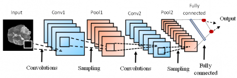
CNN is considered the most popular technique in solving image processing problems, primarily used for feature extraction purposes. The basic CNN architecture is shown in Figure 1. CNN structure comprises a convolutional layer, pooling layer, and a fully connected layer.
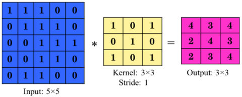
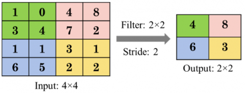
The convolutional layer is used in extracting the features of brain images with the help of filters. Figure 2 shows an example of a convolutional layer. The kernel of size 3×3 is applied over the input of size 5×5 with stride equal to one along with dot product operation and producing an output of size 3×3. The pooling layer decreases the spatial dimensions and retains the essential features of the brain images using the down-sampling technique. Figure 3 shows an example of the max-pooling layer. The filter of size 2×2 is applied over the input of size 4×4 with stride equal to two and producing an output of size 2×2 with the maximum value among the 2×2 matrix. The fully connected layer classifies the high-level features into different categories by using the softmax activation layer.
Figure 1. Basic CNN architecture
Figure 2. Convolutional layer example
Figure 3. Max-pooling layer example
3.2 Transfer learning
Transferring the knowledge, that is already gained in one area to another area for classification and feature extraction purpose is called transfer learning. The transfer learning technique is practiced in the proposed framework for classification of brain tumor. Transfer learning can be used on the pre-trained models such as AlexNet [21], ResNet [22] and, VGG [23], etc. A pre-trained network is a deep CNN model which is trained already over a huge dataset. In this method, the final layers of the pre-trained network such as Softmax activation layer and classification output layers are replaced with SVM classifier. Instead of training the entire network from scratch, we are using the already adjusted weights of the network, which is already trained on another problem. So, computation time is reduced and at the same time performance is also improved. The deep learning models are explained in the following subsections.
3.2.1 ResNet
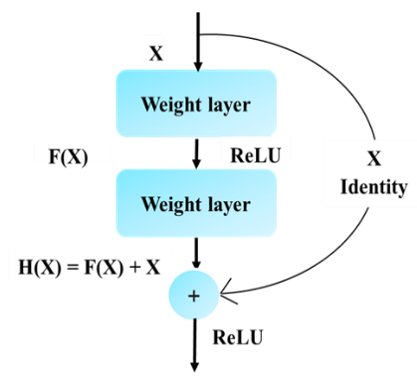
ResNet or Residual Network is one of the DCNN models. It attains good classification results by using transfer learning in various applications with improved performance. The ResNet secured first position on ImageNet Large Scale Visual Recognition Challenge (ILSVRC) and Common Objects in Context (COCO) competition in 2015. Due to the increase of layers in a deep network, a degradation problem occurs. The weights of the layer cannot be updated correctly to the next layer. To eliminate this degradation problem, ResNet uses short connections in parallel to the normal convolutional layers. The single residual building block with a short connection is shown in Figure 4. The output expression H(X) of the residual block is defined by:
H(x)=F(x)+x (1)
The stocked non- linear weight layer F(x) is given as:
F(x)=H(x)–x (2)
Figure 4. Single residual building block of ResNet
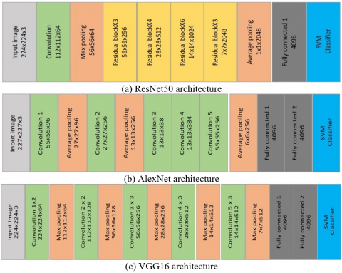
In this research, the ResNet50 model is utilized for brain tumor classification. Figure 5(a) shows the modified ResNet50 using transfer learning and consists of a 7×7 convolution layer, a 3×3 max-pooling layer, 16 residual building blocks, a 7×7 average pooling layer, a new fully-connected layer, and an SVM classifier at the last layer. The input image size for this network is 224 X 224 X 3.
3.2.2 AlexNet
AlexNet is a deep CNN architecture that secured first on the ILSVRC competition in 2012, trained on 1.2 million images with 1000 different categories using a batch size of 128 which helps to get stabilized output. Figure 5(b) shows the modified AlexNet architecture. The modified AlexNet has 5 convolutional layers, 3 max pooling layers in the original AlexNet are replaced with Average pooling layers without changing stride value, 3 fully connected layers and SVM classifier at output layer. RelU activation layer is followed by every convolutional layer.
With this modified Alexnet model, it has been observed that the training gets faster with epochs which yields the greatest performance. The input image size for this network is 227 X 227 X 3. This modified architecture was trained and validated with two different datasets with two types of classes for each of them. In the proposed framework, modified Alexnet is used as transfer learning technique by replacing 1000 classes with only 2 classes in the last layer using SVM classifier.
Figure 5. Modified pre trained DCNN architectures
3.2.3 VGGNet
VGGNet is a deep CNN architecture. It secured second place on the ILSVRC competition in 2014. The modified VGG16 model has 16 convolutional layers, 5 max-pooling layers, 3 fully connected layers, and the Softmax classifier is replaced with SVM classifier in the last layer. The RelU activation layer is followed by all fully connected layers. The input image size for this network is 224 X 224 X 3. The modified VGG16 architecture is shown in Figure 5(c).
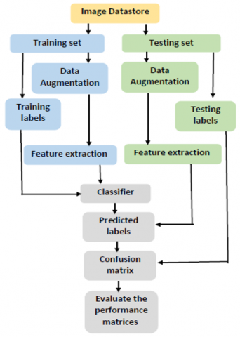
For the classification of MRI brain tumor, the dataset is collected from two different sources i.e., Kaggle and BRATS. This proposed framework is executed by training the three pre-trained architectures of the Deep Convolutional Neural network, i.e., VGG16, AlexNet, and ResNet50. During experimentation the classification is performed in three stages-preprocessing stage, feature extraction and classification. The flowchart of the proposed framework is depicted in Figure 6.
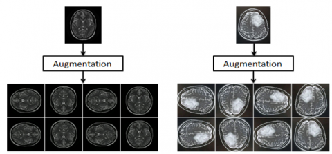
In the pre-processing stage, the collected images are resized into the input size of the pre-trained network. The image size required by AlexNet is 227 X 227 X 3, where 3 represent the number of color channels. The image size required by VGG16 and ResNet50 is 224 X 224 X 3. The pre-trained networks employ large amounts of data; if this is executed with small data, this may lead to overfitting of the network which can be avoided either with dropout layers or by using larger training dataset. In the proposed work, the data augmentation technique has been chosen to increase the data volume without muddling the pretrained architecture except the last layer. Data augmentation method helps in producing a large amount of data from the small collected data. Augmentation employs operations such as flipping, rotation, etc. to increase the volume of data. A sample image using the data augmentation technique is shown in Figure 7.
Figure 6. Flow chart of the proposed methodology
Figure 7. Sample of data augmentation technique
In the feature extraction stage, three pre-trained networks VGGNet, AlexNet, and ResNet, are used. The features are extracted from the pre-training network using the transfer learning technique. The initial layers contain low-level features, and the deeper layers have high-level features. The last fully connected layer of the network is utilized as a feature vector for extracting the features. In the modified pre-trained architecture of the proposed framework the SoftMax classification output layer is replaced with an SVM classifier for classification purpose. SVM classifier is most widely used for classification and regression purposes. In this research, Multi-class SVM is used with a linear kernel. The one-vs-all strategy is practiced in multi-class SVM classification,
The steps involved in the proposed brain tumor classification method are as follows:
Expert Radiologist involvement in the stage of segmentation and classification is required to improve the reliability of the automated tool. If we only rely on training machine to learn, there will be more chances of misdiagnosis So, therefore in our research also a professional is involved at validation stage to judge the results achieved by the methods employed during the classification (for further supervision) to avoid misdiagnosis.
5.1 Brain tumor dataset
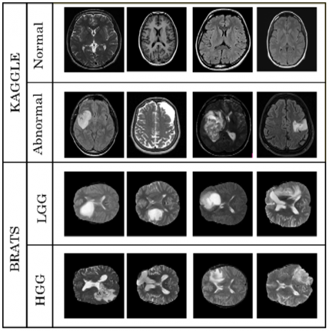
Figure 8. Samples of the dataset used
Two publicly available MRI datasets are used for validation of the proposed methodology. The first brain tumor dataset is collected from Kaggle, and the second brain tumor dataset is collected from the Multimodal Brain Tumor Image Segmentation Challenge 2015 (BRATS). Kaggle dataset contains totally 253 MRI images, where 98 of them are non-tumor (normal), and the rest 155 images are Tumor (abnormal). BRATS 2015 dataset contains 332 MRI brain images, where 156 are LGG (lower grade glioma), and the rest 176 images are HGG (higher grade glioma). The samples for the two datasets are exhibited in Figure 8. Each brain tumor dataset is parted into two sets for training and testing. The training and testing set comprises 70 percent and 30 percent, of the dataset respectively. The deep learning toolbox is used in MATLAB R2018b for the simulation.
5.2 Simulation results analysis in three phases
The proposed framework explores how the incorporation of image features besides the classifier model impacts the performance of an image classification scheme. There are three different training phases pertaining to the classifiers utilized in the last layer of the proposed brain tumor classification framework. The simulation results of this framework are progressively attained by training the framework one by one in three phases. The three phases are:(1) Training the features of deep CNN with SVM classifier, (2) Retraining the phase 1 framework with data augmentation and (3) Training the transfer learning techniques with Softmax classifier on the MR brain images.
5.2.1 Phase-1: Training the features of deep CNN with SVM classifier
In this phase, we start training all the three pre-trained models (Alexnet, Resnet and VGG16) to understand what can be attained. Initially, the detailed features are extracted from these modified pre-trained models and obtained deep features are fed to the SVM classifier by replacing the Softmax classifier present in the pre-trained model. An error-correcting output code (ECOC) model in combination of a multi-class SVM classifier is utilized in this training. In this multi-class classification, the one-vs-all approach is practiced and 3 binary SVM learners, all with kernel of type linear, have been used. Additional constraints of SVM are specified in Table 1. In this phase, the time complexity is, on an average, less than 1minute when the pre-trained models are trained since the SVM Classifier is used in the place of the Softmax classifier which is stand alone.
Table 1. Training parameters in the experiment
|
Model |
Parameters |
Settings |
|
Deep CNN with SVM Classifier |
learning factor |
|
|
|
Kernel |
BFGS |
|
|
loss function coding |
One-vs-all |
|
|
Learner |
L2 |
|
|
Model subtype |
ECOC model |
|
Deep CNN with Softmax |
Initial learning rate |
0.0002 |
|
|
Maximum Epochs |
10 |
|
|
Learning algorithm |
Adam cross Entropy |
|
|
Loss function |
10 |
|
|
Mini batch size |
20 |
5.2.2 Phase-2: Retraining the phase 1 framework with data augmentation
The framework is retrained in the second phase by adopting data augmentation. Data augmentation is a technique synthetically producing new and unique images from an existing dataset by minor alterations to the current database such as flips, translations, rotations, shears or brightness changes. It will increase the size of our training data, and our model will interpret each of these minor changes as a separate image, allowing our model to learn and function better on unseen data. Figure 7 shows a single image with many enhanced images. After retraining, the phase 1 with data augmentation, the accuracy of the framework is improved by reducing the gap between training and testing error.
5.2.3 Phase-3: Training the transfer learning techniques with Softmax classifier on the MR brain images
After pre-processing, the model's hyperparameters are computationally changed to speed up the convergence of the loss function throughout the training. Adam optimizer is used and the starting learning rate for Adam is set to 0.0002. The learning rate dictates the training period and the convergence of the optimization process. If the learning rate is more, it may avert the loss function from converging, resulting in overshoots. Contrary to it, a meagre learning rate lengthens the training period. The mini-batch size is fixed to 20. The decision involves a trade-off within the training speed (bigger batch sizes indicate faster training) and computational resources. In addition, a big batch size harms model quality. The loss function utilized is cross-entropy, which measures how close the anticipated and real distributions are. A greater learning rate at the altered FC layer is desirable to acquire the MRI image-precise features. As a result, a learning factor of ten is used. Because of the possibility of overfitting, the number of epochs used is ten. Table 1 shows the hyperparameter settings used in our simulation. In this phase, the time complexity is on an average of more than 30 minutes when the pre-trained models are trained with a Softmax classifier. The time complexity is also increased by more than 30 minutes depending on the changes done in hyperparameters during training the deep learning model.
5.3 Performance metrics and assessment
Table 2. Defining TP, FN, FP and TN
|
Definition |
Actual Label |
Predicted Label |
|
Truly Positive (TP) |
True |
True |
|
False Negative (FN) |
True |
False |
|
False Positive (FP) |
False |
True |
|
True Negative (TN) |
False |
False |
The performance of the proposed framework is measured by means of parameters such as Accuracy, Precision, Recall, Specificity, F1 score and AUC. The terms which are used to calculate the performance metrics are shown in Table 2. The Recall is the calculation of true positive ratio (TPR) values. These values measure the capacity of the framework by anticipating the right tumor types. Specificity is the calculation of true negative ratio (TNR) values, and it measures the system's capacity by classifying the negative disorder. Precision is the calculation of positive predictive rate (PPR) values. Based on Precision and Recall values F1-score is obtained. The accuracy is measured using TP and TN values.
Accuracy $=\frac{\mathrm{TP}+\mathrm{TN}}{\mathrm{TP}+\mathrm{TN}+\mathrm{FP}+\mathrm{FN}} \quad * 100$ (3)
Precision or $=\frac{\text { TP }}{T P+F P} * 100$ (4)
Recall or $\mathrm{TPR}=\frac{\mathrm{TP}}{\mathrm{TP}+\mathrm{FN}} * 100$ (5)
Specificity or TNR $=\frac{\mathrm{TN}}{\mathrm{TN}+\mathrm{FP}} * 100$ (6)
F1 Score $=2 * \frac{\text { Recall } \times \text { Precision }}{\text { Recall }+\text { Precision }} \quad * 100$ (7)
False Positive Ratio(FPR) $=\frac{F P}{F P+F N} \quad * 100$ (8)
The ROC curve is a graphical curve, that plots TPR against FPR. It is utilized to check the performance of the model. AUC is measured by using the ROC characteristics. The AUC value is ranging from 0 to 1. An AUC value of '0' specifies poor performance, and '1' indicates good performance. The AUC is calculated by using Eq. (9).
$A U C=\int_{0}^{1} \operatorname{TPR}\left(F P R^{-1}(x)\right) d x$ (9)
During classification the most widely used quality metric is Classification Accuracy. Accuracy in Classification, is measured as the proportion of appropriately classified samples divided by the whole count of data samples.
Thus the experimental results reveal that upgrade in performance is attained when an SVM classifier is trained by removing the Softmax classifier present in the pre-trained models to classify the features of deep CNN. A considerable amount of images is essential to train a neural network for sophisticated and precise results. However, our experimental results demonstrate that we can achieve full accuracy even with such a limited dataset. Our overall accuracy is very good compared to the VGG-16, ResNet-50, and Alexnet models. Our model's average training time is less than one minute, compared to around 43 minutes for the VGG-16, about 50 minutes for ResNet-50, and approximately 35 minutes for Alexnet. As a result, our framework requires fewer computational specifications (around less than 1 minute) because it needs less execution time. Furthermore, our framework outperforms VGG-16, ResNet-50, and Alexnet in terms of Accuracy also.
Features were extracted from the training and testing set using the respective DCNN model. The SVM classifier trains these models. A confusion matrix is drawn between predicted labels and test labels. Table 3 and Table 4 represents the confusion matrices of Kaggle and BRATS datasets obtained for ResNet50 using the SVM classifier. The ResNet50 model has achieved an accuracy of 98.28% and 97.87% for Kaggle and BRATS brain tumor datasets, respectively.
Table 3. Confusion matrix of Kaggle dataset using ResNet50
|
Predicted class Actual class |
Normal |
Abnormal |
|
Normal |
28 |
1 |
|
Abnormal |
0 |
29 |
Table 4. Confusion matrix of BRATS dataset using ResNet50
|
Predicted class Actual class |
LGG |
HGG |
|
LGG |
45 |
2 |
|
HGG |
0 |
47 |
5.4 Comparative analysis and discussion
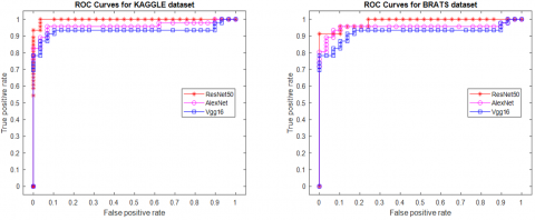
A comparison is carried out for the classification performance of VGG16, AlexNet and ResNet50 models. The transfer learning methodology is performed using VGG16, AlexNet and ResNet50 models on Kaggle and Brats datasets. VGG16 has achieved an accuracy of 91.38% for Kaggle and 90.43% for Brats brain tumor dataset, whereas AlexNet has obtained an accuracy of 94.83% for Kaggle and 94.68% for Brats brain tumor dataset. The ROC curves of Kaggle and Brats datasets using these networks is shown in Figure 9.
Table 5. Comparison of three pre-trained models using AUC
|
Dataset |
AUC |
||
|
VGG16 |
AlexNet |
ResNet50 |
|
|
KAGGLE |
0.9325 |
0.9603 |
0.9978 |
|
BRATS |
0.9235 |
0.9520 |
0.9850 |
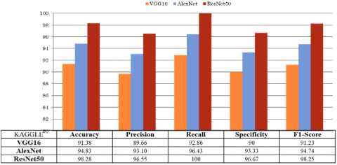
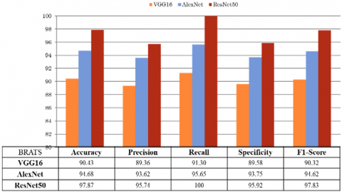
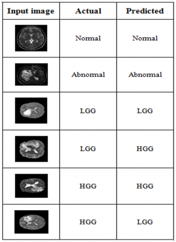
Figure 10 and Figure 11 shows the comparative analysis of the pre-trained networks on Kaggle and BRATS datasets using the confusion matrix. Table 5 shows the AUC values extracted from the ROC curves. This result indicates that among the three pre-trained models, ResNet50 achieves good performance results for both Kaggle and BRATS datasets by considering both confusion matrix and ROC characteristics. Figure 12 shows some predicted images for the unseen data using the trained model and also shows some predicted images label along with the actual label.
Figure 9. ROC curves of Kaggle and Brats datasets
Figure 10. Comparison of results obtained from different pre-trained models on Kaggle dataset using confusion matrix
Figure 11. Comparison of results obtained from different pre-trained models on BRATS dataset using confusion matrix
Figure 12. Predictions obtained for classifier
Table 6. Comparing the proposed framework with different state-of-art
|
Reference |
Feature Extraction |
Model |
Accuracy |
|
Abiwinanda et al. [3] |
Model based |
CNN |
84.19 |
|
Swati et al. [16] |
Fine-tune AlexNet |
Log-based softmax |
89.95 |
|
Fine-tune VGG16 |
94.65 |
||
|
Fine-tune VGG19 |
94.82 |
||
|
Proposed |
VGG16 |
SVM |
91.38 |
|
AlexNet |
94.83 |
||
|
ResNet50 |
98.28 |
Table 6 demonstrates the accuracy of the proposed framework against the different related methods. Swathi et al. [16] uses three trained networks such as AlexNet, VGG16, and VGG19 and achieved an accuracy of 89.95%, 94.65% and 94.82%, respectively. Fine-tuning transfer learning technique was used [16]. Abiwinanda et al. [3] proposed CNN and achieved 84.19% accuracy during validation. With these outcomes, it is proved that the proposed trained models have accomplished good Accuracy results.
In this framework, the Transfer learning process is effectively applied on the three pre-trained models-AlexNet, ResNet-50, and VGG-16 to classify the brain tumors. The performance metrics of the above three models are evaluated. The simulation results demonstrates that ResNet50 performs better in classifying brain tumor when compared with the other two networks. The proposed model comprising of Kaggle and BRATS datasets achieved a highest Classification Accuracy with less computational time after training the framework with data augmentation and SVM classifier. Therefore, this work can be successfully employed in the medical field to detect brain tumor. In future, these models can be used for in-depth classification of the tumor with more subclasses in less computational time.
[1] Jain, R., Jain, N., Aggarwal, A., Hemanth, D.J. (2019). Convolutional neural network based Alzheimer’s disease classification from magnetic resonance brain images. Cognitive Systems Research, 57: 147-159. https://doi.org/10.1016/j.cogsys.2018.12.015
[2] Yang, Y., Yan, L.F., Zhang, X., Han, Y., Nan, H.Y., Hu, Y.C., Ge, X.W. (2018). Glioma grading on conventional MR images: A deep learning study with transfer learning. Frontiers in Neuroscience, 12: 804. https://doi.org/10.3389/fnins.2018.00804
[3] Abiwinanda, N., Hanif, M., Hesaputra, S.T., Handayani, A., Mengko, T.R. (2019). Brain tumor classification using convolutional neural network. In World Congress on Medical Physics and Biomedical Engineering, 2018: 183-189. https://doi.org/10.1007/978-981-10-9035-6_33
[4] Zhang, Y., Wang, S., Ji, G., Dong, Z. (2013). An MR brain images classifier system via particle swarm optimization and kernel support vector machine. The Scientific World Journal, 2013: 130134. https://doi.org/10.1155/2013/130134
[5] Wang, S., Zhang, Y., Dong, Z., Du, S., Ji, G., Yan, J., Yang, J., Wang, Q., Feng, C., Phillips, P. (2015). Feed‐ forward neural network optimized by hybridization of PSO and ABC for abnormal brain detection. International Journal of Imaging Systems and Technology, 25(2): 153-164. https://doi.org/10.1002/ima.22132
[6] Sravan, V., Swaraja, K., Meenakshi, K., Kora, P., Samson, M. (2020). Magnetic resonance images based brain tumor segmentation-a critical survey. In 2020 4th International Conference on Trends in Electronics and Informatics (ICOEI)(48184), pp. 1063-1068. https://doi.org/10.1109/ICOEI48184.2020.9143045
[7] Ranjan Nayak, D., Dash, R., Majhi, B. (2017). Stationary wavelet transform and AdaBoost with SVM based pathological brain detection in MRI scanning. CNS & Neurological Disorders-Drug Targets (Formerly Current Drug Targets-CNS & Neurological Disorders), 16(2): 137-149.
[8] Saritha, M., Joseph, K.P., Mathew, A.T. (2013). Classification of MRI brain images using combined wavelet entropy based spider web plots and probabilistic neural network. Pattern Recognition Letters, 34(16): 2151-2156. https://doi.org/10.1016/j.patrec.2013.08.017
[9] Nayak, D.R., Dash, R., Majhi, B. (2016). Brain MR image classification using two-dimensional discrete wavelet transform and AdaBoost with random forests. Neurocomputing, 177: 188-197. https://doi.org/10.1016/j.neucom.2015.11.034
[10] Basheera, S., Ram, M.S.S. (2019). Classification of brain tumors using deep features extracted using CNN. In Journal of Physics: Conference Series, 1172(1): 012016. https://doi.org/10.1088/1742-6596/1172/1/012016
[11] Khawaldeh, S., Pervaiz, U., Rafiq, A., Alkhawaldeh, R.S. (2018). Noninvasive grading of glioma tumor using magnetic resonance imaging with convolutional neural networks. Applied Sciences, 8(1): 27. https://doi.org/10.3390/app8010027
[12] Sajjad, M., Khan, S., Muhammad, K., Wu, W., Ullah, A., Baik, S.W. (2019). Multi-grade brain tumor classification using deep CNN with extensive data augmentation. Journal of Computational Science, 30: 174-182. https://doi.org/10.1016/j.jocs.2018.12.003
[13] Carlo, R., Renato, C., Giuseppe, C., Lorenzo, U., Giovanni, I., Domenico, S., Mario, C. (2019). Distinguishing functional from non-functional pituitary macroadenomas with a machine learning analysis. In Mediterranean Conference on Medical and Biological Engineering and Computing, Springer, 76: 1822-1829. https://doi.org/10.1007/978-3-030-31635-8_221
[14] Das, S., Aranya, O.R.R., Labiba, N.N. (2019). Brain tumor classification using convolutional neural network. In 2019 1st International Conference on Advances in Science, Engineering and Robotics Technology (ICASERT), pp. 1-5. https://doi.org/10.1109/ICASERT.2019.8934603
[15] Rehman, A., Naz, S., Razzak, M.I., Akram, F., Imran, M. (2020). A deep learning-based framework for automatic brain tumors classification using transfer learning. Circuits, Systems, and Signal Processing, 39(2): 757-775. https://doi.org/10.1007/s00034-019-01246-3
[16] Swati, Z.N.K., Zhao, Q., Kabir, M., Ali, F., Ali, Z., Ahmed, S., Lu, J. (2019). Brain tumor classification for MR images using transfer learning and fine-tuning. Computerized Medical Imaging and Graphics, 75: 34-46. https://doi.org/10.1016/j.compmedimag.2019.05.001
[17] Reddy, D.J., Mounika, B., Sindhu, S., Reddy, T.P., Reddy, N.S., Sri, G.J., Swaraja, K., Meenakshi, K. and Kora, P. (2020). Predictive machine learning model for early detection and analysis of diabetes. Materials Today: Proceedings. https://doi.org/10.1016/j.matpr.2020.09.522
[18] https://www.kaggle.com/jakeshbohaju/brain-tumor, accessed on 20 March 2021.
[19] Menze, B.H., Jakab, A., Bauer, S., Kalpathy-Cramer, J., Farahani, K., Kirby, J., Lanczi, L. (2014). The multimodal brain tumor image segmentation benchmark (BRATS). IEEE Transactions on Medical Imaging, 34(10): 1993-2024. https://doi.org/10.1109/TMI.2014.2377694
[20] Kistler, M., Bonaretti, S., Pfahrer, M., Niklaus, R., Büchler, P. (2013). The virtual skeleton database: an open access repository for biomedical research and collaboration. Journal of Medical Internet Research, 15(11): e245. https://doi.org/10.2196/jmir.2930
[21] Krizhevsky, A., Sutskever, I., Hinton, G.E. (2012). ImageNet classification with deep convolutional neural networks. Communications of the ACM, 60(6): 84-90. https://doi.org/10.1145/3065386
[22] Simonyan, K., Zisserman, A. (2014). Very deep convolutional networks for large-scale image recognition. arXiv preprint arXiv:1409.1556.
[23] He, K., Zhang, X., Ren, S., Sun, J. (2016). Deep residual learning for image recognition. In Proceedings of the IEEE Conference on Computer Vision and Pattern Recognition, pp. 770-778. https://doi.org/10.1109/CVPR.2016.90