Sibghatullah I. Khan* | Ganjikunta Ganesh Kumar | Pandya Vyomal Naishadkumar | Sarvade Pedda Venkata Subba Rao
© 2021 IIETA. This article is published by IIETA and is licensed under the CC BY 4.0 license (http://creativecommons.org/licenses/by/4.0/).
OPEN ACCESS
Diagnosing chronic obstructive pulmonary disease (COPD) from lung sounds is time consuming, onerous, and subjective to the expertise of pulmonologists. The preliminary diagnosis of COPD is often based on adventitious lung sounds (ALS). This paper proposes to objectively analyze the lung sound signals associated with COPD. Specifically, empirical mode decomposition (EMD), a data adaptive signal decomposition technique suitable for analyzing non-stationary signals, was adopted to decompose non-stationary lung sound signals. The use of EMD on lung sound signal results in intrinsic mode functions (IMFs), which are symmetric and band limited. The analytic IMFs were then computed through the Hilbert transform, which reveals the instantaneous frequency content of each IMF. The Hilbert transformed signal is analytic, and has a complex representation containing real and imaginary parts. Next, the central tendency measure (CTM) was introduced to quantify the circular shape of the analytical IMF plot. The result was taken as a useful feature to distinguish normal lung sound signal with ALS. Simulation results show that the CTM of analytic IMFs has a strong ability to distinguish between normal lung sound signals and ALS.
chronic obstructive pulmonary disease (COPD), adventitious lung sounds (ALS), electronic stethoscope, intrinsic mode functions (IMFs)
Chronic respiratory diseases (CRDs) are lung and airway disorders [1]. The most common lung diseases include chronic obstructive pulmonary disease (COPD), asthma, occupational lung diseases, and pulmonary hypertension [2]. Among them, COPD is characterized by the chronic obstruction of lung airflow, which interferes with normal breathing and is not fully reversible [3]. COPD and other CRDs can be marked by the corresponding adventitious lung sound signals (ALS) [3].
The sound signals from the human lungs are very complex and highly nonlinear [4]. The parameters extracted from human lung sound signals play a critical role in ALS-based diagnosis. Time-domain parameters, including statistical features, have been used to analyze ALS [4, 5]. Assuming that lung sounds are stationary, some researchers computed spectral features through Fourier transform, and applied them to analyze and classify human lung sound signals [6, 7].
Past research reveals that the frequency components in lung sounds change over time, suggesting that the lung sound signals are non-stationary [8]. Considering this evidence, many multi-resolution methods have been proposed to detect ALS, ranging from short-time Fourier transform [9-11] and wavelet spectral analysis [12-14]. The fractal dimension has been adopted to divide ALS in multiclass classification [15, 16].
To analyze and classify lung sound signals, several methods inspired by automatic speech recognition have been explored, namely, the mel-frequency cepstral coefficients (MFCCs) classification [17-21]. There are also reports on the classification of lung sound signals based on empirical mode decomposition (EMD) [22, 23]. EMD-based analysis on electroencephalogram (EEG) signals is a hotspot. For instance, Pachori et al. [24] extracted the parameters from the respective intrinsic mode functions (IMFs), and relied on them to differentiate the EEG signals of epileptic seizure from normal EEG signals.
Drawing on previous EMD-based nonlinear signal analyses, this paper decides to analyze human lung sound signals through EMD and Hilbert-Huang transform (HHT) [25]. The Hilbert transform was applied on the IMFs of lung sound signals to obtain analytical IMFs. The IMF plots in the complex plane are circular, with each IMF reflecting its rotational frequency [26]. Therefore, circular plots have been taken as features for analyzing postural stability [27]. In this paper, the area of each circle obtained from analytic IMFs is used as a feature to distinguish between normal lung sound signals and ALS.
2.1 Dataset
This paper adopts the online database of International Conference on Brain and Health Informatics (ICBHI) 2017 [28]. This contains four sets of human lung sound signals in both normal and adventitious classes. The first set contains crackles, the second contains wheezes, the third contains both crackles and wheezes, and the fourth contains normal lung sound signals. All these sounds were recorded from 126 subjects, and labeled by respiratory experts. The recording procedures and protocols are detailed by Rocha et al. [28]. The first to third sets were combined into the class of ALS, while the fourth set was treated as the normal class.
2.2 EMD
Through EMD, any time-domain signal can be broken down into a finite number of amplitude-frequency (AM-FM) modulated oscillating components called intrinsic mode functions (IMFs) [25]. The decomposition is signal dependent, without needing any prior assumption about the stationarity and linearity of signals. For the EMD of a signal x(t), the resultant band limited IMFs must satisfy two necessary conditions: (1) the number of extrema and zero-crossings in the complete data must be the same or vary by a maximum of one; (2) in any case, the mean of the boundary specified by the extrema must be zero. The first and second conditions fulfill the narrowband requirement and elimination of redundant fluctuations due to asymmetric waveforms, respectively [25].
|
Algorithm 1 EMD algorithm of the signal x(t) |
|
1: Define g1(t)=x(t). 2: Compute all extrema of x(t). 3: Get the upper envelop em(t) and lower envelop el(t), by joining extrema through cubic spline interpolation. 4: Calculate the local mean as $m(t)=\left[e_{m}(t)+e_{l}(t)\right] / 2$. 5: Make the local mean zero by subtracting m(t) from x(t) and denoting it as d(t). 6: Apply the two necessary conditions to test whether d(t) is an IMF. 7: Iterate on d(t) and its residual. |
After calculating the first IMF, define D1(t)=g1(t), where D1(t) is the minuscule temporal scale in x(t). To derive the remaining IMFs, compute the residual signal r1(t) by subtracting D1(t) from the signal as $r_{1}(t)=x(t)-D_{1}(t)$. Repeat this process until the final residue becomes monotonic, and exists as a constant or a signal with only single minima and maxima, from which it is impossible to derive further IMFs. The extraction of IMFs and residues can be expressed as:
$r_{1}(t)-D_{2}(t)=r_{2}(t), \ldots, r_{M-1}(t)-D_{M}(t)=r_{M}(t)$ (1)
where, rM(t) is the last residue. The signal x(t) outputted by the decomposition can be expressed as:
$x(t)=\sum_{m=1}^{M} D_{m}(t)+r_{M}(t)$ (2)
where, M is the number of IMFs; Every IMF is deemed to provide a significant local frequency, and different IMFs differ in frequency. Then, formula (2) can be written as:
$x(t)=\sum_{m=1}^{M} A_{m}(t) \cos \left(\emptyset_{m}(t)\right)$ (3)
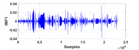
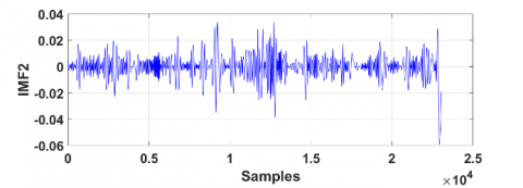
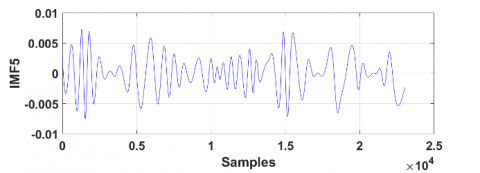
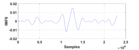
Figure 1 provides an example of the EMD on lung sound signals in two breath cycles.
Figure 1. IMFs of normal lung sound signals obtained through EMD
2.3 Hilbert transform and central tendency measure
For a real signal x(t), the Hilbert transform can be defined as:
$y(t)=x(t) * \frac{1}{\pi t}=\frac{1}{\pi} p . v \cdot \int_{-\infty}^{\infty} \frac{x(\tau)}{t-\tau} d \tau$ (4)
Through Fourier transform, we have
$Y(\omega)=-j \operatorname{sgn}(\omega) X(\omega)$ (5)
where, p.v. is the Cauchy principal value; X($\omega$) is the Fourier transform of signal x(t) [26]. Then, the analytic representation of the signal x(t) can be obtained as:
$z(t)=x(t)+j y(t)$ (6)
The analytic signal can be further expressed as:
$z(t)=A(t) e^{-j \phi(t)}$ (7)
where, $A(t)=\sqrt{x^{2}(t)+y^{2}(t)}$ is the modulus (or amplitude) of $z(t)$ and $\phi(t)=\tan ^{-1}\left(\frac{y(t)}{x(t)}\right)$ is the instantaneous phase. Differentiating instantaneous phase will result in instantaneous frequency $\omega(t)$ as:
$\omega(t)=\frac{d \phi(t)}{d t}=\frac{x(t) y(t)-x(t) y(t)}{A^{2}(t)}$ (8)
where, $\omega(t)$ is an instantaneous frequency reflecting the rotation rate of the analytic signal in the complex plane.
Considering the local symmetry of IMFs, localized instantaneous frequency can be obtained in the spectro-temporal domain, revealing the essential features of the signal [25]. From formula (3), each IMF $D_{m}(t)=A_{m}(t) \cos \phi_{m}$ can be represented analytically as:
$Z_{m}(t)=A_{m} e^{-j \phi_{m}(t)}$ (9)
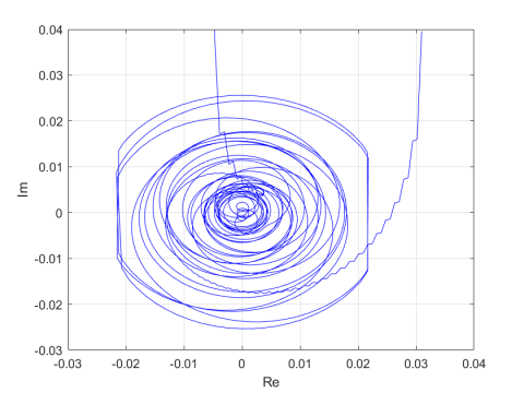
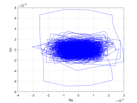
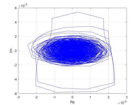
Figures 2 and 3 provide examples of analytic signal plots in a complex plane for the first four IMFs. In nature, these plots are similar to rotating curves with a proper structure and a unique center. Our research mainly attempts to discriminate between natural lung signals and ALS, using the circular shape of analytical IMFs in a complex plane. To accomplish this goal, the CTM was introduced to the computation of feature set.
The CTM provides a way to summarize the visual information contained in the plots [29]. In previous studies, the CTM of second-order difference plots (SODPs) have been utilized to compute the degree of variability in EEG and the center of pressure signals [30, 31]. In this paper, the CTM is adopted to calculate the area parameter of each circular analytic IMF. Specifically, the radius was computed by including more than 95% traces of the CTM. The z(n) was represented analytically by plotting the imaginary part of z(n), i.e., $A(n) \sin \phi(n)$, with its real part, i.e., $A(n) \cos \phi(n)$.
The analytic depiction of the signal meets two criteria: each plot rotates in a specific direction; each plot has a unique center. In case of non-stationary signals, these two criteria cannot be fulfilled, because a non-stationary signal rotates about multiple centers. The IMFs obtained through EMD define the complex non-stationary signal as the sum of unique proper rotations, thereby determining the area of analytical IMF in the complex plane.
The CTM was computed by choosing a circular area of radius r around the origin. Then, the number of points within the radius was counted, and divided by the sum of the total points [29]. Let N be the sum of total points; r be the corresponding radius. Then, the CTM of analytic signal z(n) can be computed by:
$C T M=\frac{\sum_{n=1}^{N} \delta\left(d_{n}\right)}{N}$ (10)
where, δ(dn) can be given as:
$\delta\left(d_{n}\right)=\left\{\begin{array}{l}1, &{if \left([\Re\{z[n]\}]^{2}+[\Im\{z[n]\}]^{2}\right)<r} \\ 0, &{otherwise}\end{array}\right.$ (11)
$\delta\left(d_{n}\right)$ represents the nth point inside the radius r. The radius r was chosen such that it covers 95% of the total points in the SODP plot. Further information about the CTM measure can be obtained in the study [29]. For each radius r, the corresponding CTM represents the fraction of a total number of points included in the circle. Figures 2 and 3 provide the CTM plots of the first two IMFs of normal lung sound signals and ALS, respectively.
(a)
(b)
(c)
(d)
(e)
Figure 2. Analytic signal representations on complex plane: (a) Normal lung sound signals (b) IMF1, (c) IMF2, (d) IMF3, and (e) IMF4
(a)
(b)
(c)
(d)
(e)
Figure 3. Analytic signal representations on complex plane: (a) ALS (b) IMF1, (c) IMF2, (d) IMF3, and (e) IMF4
In this paper, EMD is implemented prior to Hilbert transform. This approach offers greater insight than the direct application of Hilbert transform on the entire signal. In this way, substantial variations were found in the surface area of normal lung sound signals and ALS. Figures 2(a) and 3(a) provide the analytic representation of normal lung sound signals and ALS. Significant difference can be observed between the two classes of signals. In addition, the analytic representation of IMFs of respective class shows a marked difference between normal lung sound signals and ALS. The upper and lower ranges of x and y axis can give the idea of amplitude variations. For example, the x and y ranges of normal lung sound signal were (-0.4, +0.4), while those of ALS were (-1, +1.5). Similar differences were observable for their IMFs as well.
From Figures 2 and 3, it can be observed that the analytic representation of lung sound signals does not depict any specific pattern or geometry in the complex plane. Consequently, it is inconvenient to define the radius of a circle that includes more than 95% of the total data points. The multiple rotation centers in Figures 2(a) suggest the presence of several distinct frequency components in the lung sound signals. In contrast, the analytic signals obtained through EMD of IMF covered more than 95% of the data points in the complex plane that rests within a circle. Moreover, these forms of analytic traces differed between normal lung sound signals and ALS. Since each IMF is always circular (Figures 2(b)-(e) and Figures 3(b)-(e)), it is feasible to measure the surface area in the complex plane. In this paper, the estimated area of analytic IMFs is treated as a feature to discriminate between normal lung sound signals and ALS.
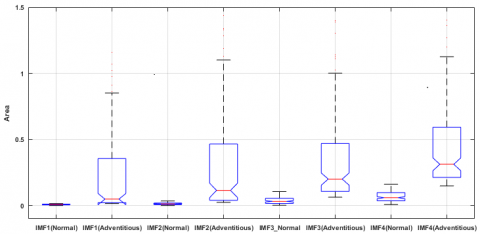
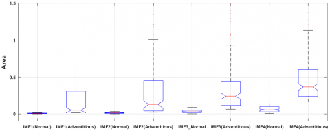
As mentioned before, the first to third sets of the ICBHI database were combined into the class of ALS, and the fourth set was used as the class of normal lung sound signals. For the said classes, the area parameters were determined using the analytical representation of IMFs for different window sizes (N=40,000, 50,000, 60,000, and 70,000 samples). Table 1 lists the area parameters [minimum(min), median(med), and maximum(max)] for each IMF class with different window sizes. The estimated maximum area of ALS was larger than that of normal lung sound signals. A possible reason is the relatively large amplitude and different frequency contents of all IMFs.
Next, the class discriminating potential of the area feature was assessed by the Kruskal-Wallis statistical test. The area values were remarkably distinct between the two classes of signals (p=0.001).
Figures 4-7 display the results of the first four IMFs of different window sizes. The results indicate the effectiveness of the surface area of analytic IMFs in discriminating normal lung sound from ALS. The utilization of EMD is justified as there was no specific geometry or unique center of rotation for the analytic representation of the complete signal. Through the EMD, the analytic IMFs were mapped into a complex plane with circular geometry and a unique center. This method resulted in viability in the area computation of analytic IMFs, which covers more than 95% of the total data points. In future research, the circle area threshold for discriminating normal lung sound signals and ALS can be suggested, using a larger out-of-sample dataset.
Table 1. Analytic IMFs area for normal adventitious lung sound signals
|
Subject |
Window Size |
IMF1 |
IMF2 |
IMF3 |
IMF4 |
||||||||
|
Min |
Med |
Max |
Min |
Med |
Max |
Min |
Med |
Max |
Min |
Med |
Max |
||
|
Normal Lung sound signals |
40000 |
0.00 |
0.00 |
0.01 |
0.00 |
0.01 |
0.03 |
0.00 |
0.03 |
0.10 |
0.00 |
0.06 |
0.16 |
|
50000 |
0.00 |
0.00 |
0.01 |
0.00 |
0.01 |
0.03 |
0.00 |
0.02 |
0.09 |
0.00 |
0.05 |
0.16 |
|
|
60000 |
0.00 |
0.00 |
0.01 |
0.00 |
0.01 |
0.02 |
0.00 |
0.02 |
0.09 |
0.00 |
0.06 |
0.16 |
|
|
70000 |
0.00 |
0.00 |
0.01 |
0.00 |
0.00 |
0.03 |
0.00 |
0.02 |
0.08 |
0.00 |
0.05 |
0.16 |
|
|
Adventitious Lung sound signals |
40000 |
0.00 |
0.01 |
4.43 |
0.00 |
0.02 |
2.81 |
0.00 |
0.06 |
4.72 |
0.00 |
0.13 |
3.11 |
|
50000 |
0.00 |
0.01 |
4.28 |
0.00 |
0.02 |
3.27 |
0.00 |
0.06 |
4.14 |
0.00 |
0.15 |
2.92 |
|
|
60000 |
0.00 |
0.01 |
3.94 |
0.00 |
0.01 |
3.31 |
0.00 |
0.05 |
3.50 |
0.00 |
0.15 |
3.15 |
|
|
70000 |
0.00 |
0.01 |
3.58 |
0.00 |
0.01 |
3.15 |
0.00 |
0.05 |
2.88 |
0.00 |
0.12 |
3.09 |
|
Figure 4. Comparison of area parameters between IMF1 (p=0.001), IMF2 (p= 0.001), IMF3 (p= 0.001), and IMF4 (p= 0.001) of normal lung sound signals and ALS (window length= 40,000 samples)
Figure 5. Comparison of area parameters between IMF1 (p<0.001), IMF2 (p<0.001), IMF3 (p<0.001), and IMF4 (p<0.001) of normal lung sound signals and ALS (window length= 50,000 samples)
Figure 6. Comparison of area parameters between IMF1 (p=0.001), IMF2 (p= 0.001), IMF3 (p= 0.001), and IMF4 (p= 0.001) of normal lung sound signals and ALS (window length= 60,000 samples)
Figure 7. Comparison of area parameters between IMF1 (p=0.001), IMF2 (p= 0.001), IMF3 (p= 0.001), and IMF4 (p= 0.001) of normal lung sound signals and ALS (window length= 70,000 samples)
This paper investigates the ability of the analytic IMFs to discriminate normal lung sound signals and ALS. The application of EMD to decompose lung sound signals is an encouraging method that provides proper circular structures of analytical IMFs in a complex plane. A significant statistical difference was observed between normal lung sound signals and ALS. The latter had a much larger area of analytic IMF than normal lung sound signal. This is potentially due to the relatively high amplitude and variable frequency of ALS. Moreover, the EMD provided a unique center of rotation for each analytic IMF. The clinical diagnostic ability of the proposed method needs to be tested on out of sample dataset. One exciting area of future research could be examining the feasibility of the area measure of analytic IMFs in classifying normal, crackles, and wheezing lung sound signals.
[1] Sovijärvi, A.R.A., Malmberg, L.P., Charbonneau, G., Vandershoot, J. (2000). Characteristics of breath sounds and adventitious respiratory sounds. European Respiratory Review, 10(77): 591-596.
[2] Sovijarvi, A.R.A., Dalmasso, F., Vanderschoot, J., Malmberg, L.P., Righini, G., Stoneman, S.A. (2000). Definition of terms for applications of respiratory sounds. European Respiratory Review, 10(77): 597-610.
[3] Pasterkamp, H., Kraman, S.S., Wodicka, G.R. (1997). Respiratory sounds, advances beyond the stethoscope. American Journal of Respiratory and Critical Care Medicine, 156(3): 974-87. https://doi.org/10.1164/ajrccm.156.3.9701115
[4] Reichert, S., Gass, R., Brandt, C., Andrès, E. (2008). Analysis of respiratory sounds: state of the art. Clin Med Circ Respirat Pulm Med., 2: 45-58. https://doi.org/10.4137/ccrpm.s530
[5] Murphy, R.L., Vyshedskiy, A., Power-Charnitsky, V., Bana, D., Marinelli, P., Wong-Tse, A., Paciej, R. (2003). Automated lung sound signals analysis in patients with pneumonia. Chest, 124(4): 190S. https://doi.org/10.1378/chest.124.4_MeetingAbstracts.190S-b
[6] Oud, M., Dooijes, E.H., van der Zee, J.S. (2000). Asthmatic airways obstruction assessment based on detailed analysis of respiratory sound spectra. IEEE Transactions on Biomedical Engineering, 47(11): 1450-1455. https://doi.org/10.1109/10.880096
[7] Waitman, L.R., Clarkson, K.P., Barwise, J.A., King, P.H. (2000). Representation and classification of breath sounds recorded in an intensive care setting using neural networks. Journal of Clinical Monitoring and Computer, 16: 95-105. https://doi.org/10.1023/A:1009934112185
[8] İçer, S., Gengeç, S. (2014). Classification and analysis of non-stationary characteristics of crackle and rhonchus lung adventitious sounds. Digital Signal Processing, 28: 18-27. https://doi.org/10.1016/j.dsp.2014.02.001
[9] Niu, J., Cai, M., Shi, Y., Ren, S., Xu, W., Gao, W., Luo, Z., Reinhardt, J.M. (2019). A novel method for automatic identification of breathing state. Scientific Reports, 9: 103. https://doi.org/10.1038/s41598-018-36454-5
[10] Morillo, D.S., Jiménez, A.L., Moreno, S.A. (2013). Computer-aided diagnosis of pneumonia in patients with chronic obstructive pulmonary disease. Journal of the American Medical Informatics Association, 20(e1): e111-e117. https://doi.org/10.1136/amiajnl-2012-001171
[11] Riella, R.J., Nohama, P., Maia, J.M. (2009). Method for automatic detection of wheezing in lung sound signals. Brazilian Journal of Medical and Biological Research, 42(7): 674-684. https://doi.org/10.1590/S0100-79X2009000700013
[12] Kandaswamy, A., Kumar, C.S., Ramanathan, R.P., Jayaraman, S., Malmurugan, N. (2004). Neural classification of lung sound signals using wavelet coefficients. Computers in Biology and Medicine, 34(6): 523-37. https://doi.org/10.1016/S0010-4825(03)00092-1
[13] Shi, Y., Li, Y., Cai, M., Zhang, X.D. (2019). A lung sound signals category recognition method based on wavelet decomposition and BP neural network. International Journal of Biological Science, 15(1): 195‐207. https://doi.org/10.7150/ijbs.29863
[14] Abougabal, M.M., Moussa, N.D. (2018). A novel technique for validating diagnosed respiratory noises in infants and children. Alexandria Engineering Journal, 57(4): 3033-3041. https://doi.org/10.1016/j.aej.2018.05.003
[15] Rizal, A., Hidayat, R., Nugroho, H.A. (2018). Fractal dimension for lung sound signals classification in multiscale scheme. Journal of Computer Science, 14: 1081-1096. https://doi.org/10.3844/jcssp.2018.1081.1096
[16] Reljin, N., Reyes, B.A., Chon, K.H. (2015). Tidal volume estimation using the blanket fractal dimension of the tracheal sounds acquired by smartphone. Sensors (Basel), 15(5): 9773-9790. https://doi.org/10.3390/s150509773
[17] Bahoura, M. (2009). Pattern recognition methods applied to respiratory sounds classification into normal and wheeze classes. Computers in Biology and Medicine, 39(9): 824-843. https://doi.org/10.1016/j.compbiomed.2009.06.011
[18] Sengupta, N., Sahidullah, M., Saha, G. (2016). Lung sound signals classification using cepstral-based statistical features. Computers in Biology and Medicine, 75: 118-129. https://doi.org/10.1016/j.compbiomed.2016.05.013
[19] Palaniappan, R., Sundaraj, K. (2013). Respiratory sound classification using cepstral features and support vector machine. 2013 IEEE Recent Advances in Intelligent Computational Systems (RAICS), Trivandrum, pp. 132-136. https://doi.org/10.1109/RAICS.2013.6745460
[20] Aras, S., Gangal, A. (2017). Comparison of different features derived from mel frequency cepstrum coefficients for classification of single channel lung sound signals. 2017 40th International Conference on Telecommunications and Signal Processing (TSP), Barcelona, pp. 346-349. https://doi.org/10.1109/TSP.2017.8076002
[21] Khan, S.I., Jawarkar, N.P., Ahmed, V. (2012). Cell phone based remote early detection of respiratory disorders for rural children using modified stethoscope. 2012 International Conference on Communication Systems and Network Technologies, Rajkot, pp. 936-940. https://doi.org/10.1109/CSNT.2012.199
[22] Rizal, A., Hidayat, R., Nugroho, H.A. (2017). Lung sound signals classification using empirical mode decomposition and the Hjorth descriptor. American Journal of Applied Sciences, 14(1): 166-173. https://doi.org/10.3844/ajassp.2017.166.173
[23] Lozano, M., Fiz, J.A., Jané, R. (2016). Automatic differentiation of normal and continuous adventitious respiratory sounds using ensemble empirical mode decomposition and instantaneous frequency. IEEE Journal of Biomedical and Health Informatics, 20(2): 486-497. https://doi.org/10.1109/JBHI.2015.2396636
[24] Pachori, R.B., Bajaj, V. (2011). Analysis of normal and epileptic seizure EEG signals using empirical mode decomposition, Computer Methods and Programs in Biomedicine, 104(3): 373-381. https://doi.org/10.1016/j.cmpb.2011.03.009
[25] Huang, N.E., Shen, Z., Long, S.R., Wu, M.C., Shih, H.H., Zheng, Q., Yen, N.C., Tung, C.C., Liu, H.H. (1998). The empirical mode decomposition and Hilbert spectrum for nonlinear and non-stationary time series analysis. Proceeding of the Royal Society of London Series A, 454: 903-995. https://doi.org/10.1098/rspa.1998.0193
[26] Lai, Y.C., Ye, N. (2003). Recent developments in chaotic time series analysis. International Journal of Bifurcation and Chaos, 13(6): 1383-1422. https://doi.org/10.1142/S0218127403007308
[27] Amoud, H., Snoussi, H., Hewson, D.J., Duchene, J. (2007). Hilbert-Huang transformation: Application to postural stability analysis. Proceedings of the 29th IEEE EMBS Annual International Conference, Lyon, France. https://doi.org/10.1109/IEMBS.2007.4352602
[28] Rocha, B.M., Filos, D., Mendes, L., Serbes, G., Ulukaya, S., Kahya, Y.P., Jakovljevic, N., Turukalo, T.L., Vogiatzis, I.M., Perantoni, E., Kaimakamis, E., Natsiavas, P., Oliveira, A., Jácome, C., Marques, A., Maglaveras, N., Paiva, R.P., Chouvarda, I., de Carvalho, P. (2019). An open access database for the evaluation of respiratory sound classification algorithms. Physiological Measurement, 40: 035001 https://doi.org/10.1088/1361-6579/ab03ea
[29] Cohen, M.E., Hudson, D.L., Deedwania, P.C. (1996). Applying continuous chaotic modeling to cardiac signal analysis. IEEE Engineering in Medicine and Biology Magazine, 15(5): 97-102. https://doi.org/10.1109/51.537065
[30] Thuraisingham, R.A., Tran, Y., Boord, P., Craig, A. (2007). Analysis of eyes open, eye closed EEG signals using second-order difference plot. Medical & Biological Engineering & Computing, 45(12): 1243-1249. https://doi.org/10.1007/s11517-007-0268-9
[31] Pachori, R.B., Hewson, D., Snoussi, H., Duchene, J. (2009). Postural time-series analysis using empirical mode decomposition and second-order difference plots. Proceedings IEEE International Conference on Acoustics, Speech, and Signal Processing, Taipei, Taiwan, pp. 537-540. https://doi.org/10.1109/ICASSP.2009.4959639