Yujie He
© 2021 IIETA. This article is published by IIETA and is licensed under the CC BY 4.0 license (http://creativecommons.org/licenses/by/4.0/).
OPEN ACCESS
With the advancement of artificial intelligence (AI) and the upgrading of intelligent manufacturers, the development of intelligent manufacturing is now propelled by the replacement of inefficient traditional assembly machines and operators with machine vision (MV)-based industrial robots. The classic job recognition and positioning algorithm has multiple shortcomings, such as high complexity, manual design of similarity function, and susceptibility to noise disturbance. To solve these shortcomings, this study presents a fast job recognition and sorting method based on image processing. Firstly, the extraction approach for wavelet moment features and wavelet descriptors was introduced, and the feature fusion based on echo state network (ESN) was detailed. Then, the authors explained the idea of job template matching, and described how to measure similarity and terminate the measurement during template matching. Experimental results fully manifest the effectiveness of our strategy for fast job recognition and sorting. Our method offers a new solution to rapid recognition and sorting of objects in other fields.
image processing, fast job recognition, job sorting, echo state network (ESN)
The traditional shop with a single machine cannot efficiently process the various kinds of parts involved in the multi-type small-batch production model [1-4]. With the advancement of artificial intelligence (AI) and the upgrading of intelligent manufacturers, the development of intelligent manufacturing is now propelled by the replacement of inefficient traditional assembly machines and operators with machine vision (MV)-based industrial robots [5-7]. The MV-based industrial robot system has three prominent advantages: high recognition and sorting precision, stable and continuous working state, and adaptability to complex working conditions [8-10]. Therefore, it is of certain practical significance to analyze the job recognition and sorting strategy of the MV-based industrial robot sorting system.
Image processing makes it faster and smarter to complete tasks [11-15]. Ali and Ali [16] established global mathematical models and transform matrices for the coordinate system of industrial robot, industrial camera, and the target job, processed the preprocessed job images through template matching, Canny edge feature extraction, and contour moment, and transmitted the obtained coordinates of the target job to industrial robot control system. Kothuru et al. [17] designed a waste plastics recycling and sorting system, which realizes the feature extraction, judgement, and recognition of waste plastics in different colors; such waste plastics are sorted with the aid of relays and high-speed compressed air nozzles. Their system reduces the misclassification rate to as low as 4.5%.
The classic processing method for image point cloud cannot effectively recognize the jobs of complex shapes under micro environmental interferences [18-23]. For two-dimensional (2D) job images of different scales and poses, Gutt [24] constructed a 2D convolutional neural network (CNN) for the detection of weld jobs, and introduced a transform network capable of autonomous learning to adapt the CNN to the changing poses of the target job. Nishiyama et al. [25] established a CNN applicable to three-dimensional (3D) job point cloud rotating by different angles, realized the autonomous learning of rotation parameters with a transform network and a hierarchical feature extraction network, and effectively improved the mean classification rate in network tests. Facing the insufficiency of job class and attribute samples, Tsai and Hocheng [26] proposed a method to automatically construct the input dataset for deep CNN and label the samples: the multi-view target job dataset was generated rapidly according to illumination transform, using the multi-view multi-source image fusion algorithm; then, the point cloud data went through format conversion, up-sampling, and data enhancement, producing a 3D job point cloud dataset that satisfies the training demand of deep neural network. The actual job images are prone to have problems like weak textures and motion blur. Labbi et al. [27] combined the edge fusion algorithms for color images and depth images, trying to effectively complete and connect the fused edge images of the target job. Their 3D job detection network successfully weakens the impact of image background point cloud data on the recognition rate of job point cloud data.
The above algorithms can recognize and position the target job to different degrees. However, they have shortcomings like high complexity, manual design of similarity function, and susceptibility to noise disturbance. Fortunately, the job recognition algorithm based on artificial neural network (ANN) is capable of autonomous learning and discriminative expression. Therefore, this paper proposes a fast job recognition and sorting method based on image processing. The main contents of this work are as follows: (1) presenting the extraction strategy for wavelet moment features and wavelet descriptors; (2) detailing the feature fusion based on echo state network (ESN); (3) providing the idea of job template matching; (4) explaining the similarity measurement and its termination during template matching. The proposed fast job recognition and sorting method was proved effective through experiments.
2.1 Extraction of wavelet moment features and wavelet descriptors
Let hc(ρ) and rieω be the radial component of polar diameter ρ and the and angular component rieω of polar angle ω, respectively. Then, the moment in the polar coordinate system can be defined as:
${{J}_{ce}}=g\left( \rho ,\omega \right){{h}_{c}}\left( \rho \right){{r}^{-ic\omega }}\rho d\rho d\omega $ (1)
Let NS and MT be the scale factor and the translation factor, respectively. Then, the wavelet function family in the polar coordinate system can be defined as:
${{\Phi }_{{{N}_{S}},{{M}_{T}}}}\left( \rho \right)={{N}_{S}}^{-\frac{1}{2}}\Phi \left( \frac{\rho -{{M}_{T}}}{{{N}_{S}}} \right)$ (2)
Under different frequency components, the features of the wavelet function family depend on the discrete integer form of NS and MT. Substituting hc(ρ) in formula (1) with ΦNS,MT(ρ), the wavelet moment can be obtained as:
${{Q}_{{{N}_{S}},{{M}_{T}},e}}=\int{{{R}_{e}}\left( \rho \right)}{{\Phi }_{{{N}_{S}},{{M}_{T}}}}\left( \rho \right)\rho d\rho $ (3)
where, Re(ρ) is the e-th feature in the [0, 180°] phase space:
${{R}_{e}}\left( \rho \right)=\int{g\left( \rho ,\omega \right)}{{r}^{-ie\omega }}d\omega $ (4)
The NS value is 0, 1, 2, …, and the MT value is 0, 1, 2, ..., 2NS-1. After rotating by angle β, the moment feature of the job image remains constant. Thus, we have:
$\begin{align} & Q_{{{N}_{S}},{{M}_{T}},e}^{*}=g\left( \rho ,\omega \right){{\Phi }_{{{N}_{S}},{{M}_{T}}}}\left( \rho \right){{r}^{-ie\left( \omega +\beta \right)}}\rho d\rho d\omega \\ & ={{Q}_{{{N}_{S}},{{M}_{T}},e}}{{r}^{-ie\beta }} \\\end{align}$ (5)
Modulating the left and right terms of formula (5) simultaneously, i.e., ||QNS, MT, e*||=||QNS, MT, er-ieβ||=||QNS, MT, e||, the rotation invariance of wavelet moment can be verified.
To build a wavelet moment for fast job recognition, it is necessary to compare and select wavelet functions Φu,v(ρ), under the constraint of taking non-zero values only in a finite set. Then, the generating function must be a compactly supported cubic B-spline wavelet with good locality in both time and frequency domains:
$\begin{align} & \Phi \left( \rho \right)=\frac{4{{\beta }^{{{M}_{T}}+1}}}{\sqrt{2\pi \left( {{M}_{T}}+1 \right)}}{{\varepsilon }_{Q}}cos\left( 2\pi {g}'\left( 2\rho -1 \right) \right) \\ & exp\left( -\frac{{{\left( 2\rho -1 \right)}^{2}}}{2\varepsilon _{Q}^{2}\left( {{M}_{T}}+1 \right)} \right) \\\end{align}$ (6)
where, MT=3; β=0.7; g'=0.41; ε2Q=0.56. In actual working conditions, the size, location, and other attributes of the job image, as well as their feature values, change with the shooting environment. The wavelet moment is not invariant during translation and scaling. To keep image feature descriptors invariant to translation and scaling, the feature extraction of the job image should be preceded by normalization, polar coordinate transform, and discretization.
Let us denote scale coefficient and wavelet coefficient as <g(τ), ΦI, MT(τ)> and <g(τ), Φi, MT(τ)>. The wavelet transform of continuous periodic signal g(τ) belong to K2(0, 1) can be expressed as:
$\begin{align} & g\left( \tau \right)=\sum\limits_{{{M}_{T}}}{<g\left( \tau \right),}{{\Phi }_{I,{{M}_{T}}}}\left( \tau \right)>{{\Phi }_{I,{{M}_{T}}}}\left( \tau \right) \\ & +\sum\limits_{i}^{I}{\sum\limits_{{{M}_{T}}}{<g\left( \tau \right)}},{{\Phi }_{i,{{M}_{T}}}}\left( \tau \right)>{{\Phi }_{i,{{M}_{T}}}}\left( \tau \right) \\\end{align}$ (7)
Formula (7) shows that the first and second terms on the right side of the equal sign correspond to the low- and the high-frequency parts of g(τ), respectively. The two parts correspond to the approximate representation of g(τ) at scale I and the increased details of g(τ), respectively. The scale function of g(τ) can be defined by:
${{\Phi }_{I,{{M}_{T}}}}\left( \tau \right)=\sum\limits_{k\in C}{{{\Phi }_{I,{{M}_{T}}}}\left( \tau +1 \right)}$ (8)
The wavelet function of g(τ) can be defined by:
${{\Phi }_{i,{{M}_{T}}}}\left( \tau \right)=\sum\limits_{k\in C}{{{\Phi }_{I,{{M}_{T}}}}\left( \tau +1 \right)}$ (9)
The wavelet transform of the discrete periodic signal corresponding to g(τ) can be described as:
$\begin{align} & g\left( l \right)=\sum\limits_{{{M}_{T}}}{<g\left( l \right),}{{\Phi }_{I,{{M}_{T}}}}\left( \tau \right)>{{\Phi }_{I,{{M}_{T}}}}\left( \tau \right) \\ & +\sum\limits_{i}^{I}{\sum\limits_{{{M}_{T}}}{<g\left( l \right)}},{{\Phi }_{i,{{M}_{T}}}}\left( l \right)>{{\Phi }_{i,{{M}_{T}}}}\left( l \right) \\\end{align}$ (10)
If there exists a sequence of the planar contours of job image C(l)=[a(l),b(l)]T, l=0, 1, 2, …, and if the discrete periodic sequence C(l) satisfies C(l)=C(l+1). The wavelet transform of C(l) can be performed as:
$\left[\begin{array}{l}a(l) \\ b(l)\end{array}\right]=\left[\begin{array}{l}<a(l), \Phi_{L M_{T}}(\tau)> \\ <b(l), \Phi_{L M_{T}}(\tau)>\end{array}\right] \Phi_{I, M_{\tau}}(\tau)$$+\left[\begin{array}{l}<a(l), \Phi_{i, M_{T}}(\tau)> \\ <b(l), \Phi_{j, M_{T}}(\tau)>\end{array}\right] \Phi_{i, M_{T}}(\tau)$ (11)
Then, Canny edge detector was adopted to extract the edge of the target job from the job image, that is, segment the gray image of the job and obtain the corresponding binary image. After that, the Euclidean distances of the edge pixels to the job center were calculated and sorted. Finally, the Euclidean distance sequence was depicted by a wavelet descriptor. Let K be the length of the job edge; MP be the number of pixels sampled from the edge at an interval of K/MP. Then, the sampled pixel set can be expressed as O={(a1, b1), (a2,b2), …, (aMP,bMP)}; the job center coordinates can be described as (a*, b*). The value of (a*, b*) can be calculated by the Green’s formula. The a* value can be described by:
${{a}^{*}}=\frac{\oint\limits_{a,b\in O}{\left( abda-\frac{1}{2}{{a}^{2}}bdb \right)}}{\oint\limits_{a,b\in O}{\left( bda-adb \right)}}$ (12)
The b* value can be described by:
${{b}^{*}}=\frac{\oint\limits_{a,b\in O}{\left( \frac{1}{2}{{b}^{2}}da-abdb \right)}}{\oint\limits_{a,b\in O}{\left( bda-adb \right)}}$ (13)
The discretized aD* can be described by:
$a_{D}^{*}=\frac{\sum\limits_{l=0}^{{{M}_{P}}-1}{\left[ {{b}_{l}}\left( a_{l}^{2}-a_{l-1}^{2} \right)-a_{l}^{2}\left( {{b}_{l}}-{{b}_{l-1}} \right) \right]}}{2\sum\limits_{l=0}^{{{M}_{P}}-1}{\left[ {{b}_{l}}\left( {{b}_{l}}-{{b}_{l-1}} \right)-{{a}_{l}}\left( {{b}_{l}}-{{b}_{l-1}} \right) \right]}}$ (14)
The discretized bD* can be described by:
$b_{D}^{*}=\frac{\sum\limits_{l=0}^{{{M}_{P}}-1}{\left[ b_{l}^{2}\left( {{a}_{l}}-{{a}_{l-1}} \right)-{{a}_{l}}\left( b_{l}^{2}-b_{l-1}^{2} \right) \right]}}{2\sum\limits_{l=0}^{{{M}_{P}}-1}{\left[ {{b}_{l}}\left( {{a}_{l}}-{{a}_{l-1}} \right)-{{a}_{l}}\left( {{b}_{l}}-{{b}_{l-1}} \right) \right]}}$ (15)
The Euclidean distance sequence dl from the edge pixels to job center can be described as:
${{d}_{l}}=\sqrt{{{\left( {{a}_{l}}-a_{D}^{*} \right)}^{2}}+{{\left( {{b}_{l}}-b_{D}^{*} \right)}^{2}}}$ (16)
Let dmax be the maximum of the Euclidean distance sequence dl= (d1, d2, d3, …, dMP) after normalization. To reduce the impact of image size on job recognition effect, it is necessary to normalize the dl by dj /dmax, j= 0, 1, …MP, aiming to control the elements of dl within (0, 1).
Then, the error comparison was carried out on edge features. Let J10, J20, and J30 be the wavelet descriptors composed of 10, 20, and 30 wavelet coefficient points that can be extracted from the edge image of the target job after three-layer wavelet decomposition, respectively. Due to the symmetry of the job image to be recognized, the center-edge distance sequence of the job before and after wavelet reconstruction can be denoted as dD(l) and d'D(l), respectively. Then, the error of job edge reconstructed by Coilfet wavelet basis against the sample edge can be calculated by:
$Error=\frac{{{\sum\limits_{l=0}^{{{M}_{P}}-1}{\left[ {{d}_{D}}\left( l \right)-{{d}_{D}}\left( l \right) \right]}}^{2}}}{\sum\limits_{l=0}^{{{M}_{P}}-1}{d_{D}^{2}\left( l \right)}}$ (17)
2.2 Feature fusion
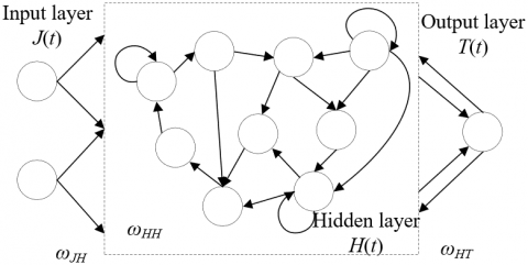
In image processing, the ESN is superior to other neural networks in that the connections between hidden layer neurons are immune to artificial disturbance, in addition to its small training load and short-term memory ability. Figure 1 shows the structure of the ESN. Let NJ, NH, and NT be the number of neurons in the three layers of the ESN; J(t), H(t), and T(t) be the input vectors of the three layers of the ESN. Then, the network in the t-th iteration can be expressed as:
$\left\{ \begin{align} & J\left( t \right)={{\left( {{J}_{1}}\left( t \right),{{J}_{2}}\left( t \right),..,{{J}_{{{N}_{J}}}}\left( t \right) \right)}^{T}} \\ & H\left( t \right)={{\left( {{H}_{1}}\left( t \right),{{H}_{2}}\left( t \right),..,{{H}_{{{N}_{H}}}}\left( t \right) \right)}^{T}} \\ & T\left( t \right)={{\left( {{T}_{1}}\left( t \right),{{T}_{2}}\left( t \right),..,{{T}_{{{N}_{T}}}}\left( t \right) \right)}^{T}} \\ \end{align} \right.$ (18)
Figure 1. ESN structure
The weight matrix ωJH between input layer and hidden layer can be expressed as:
${{\omega }_{JH}}=\left[ \begin{align} & \omega _{11}^{JH}\text{ }\omega _{12}^{JH}\text{ }...\text{ }\omega _{1{{N}_{H}}}^{JH} \\ & \omega _{21}^{JH}\text{ }\omega _{22}^{JH}\text{ }...\text{ }\omega _{2{{N}_{H}}}^{JH} \\ & \text{ }...\text{ }...\text{ }...\text{ }... \\ & \omega _{{{N}_{J}}1}^{JH}\text{ }\omega _{{{N}_{J}}2}^{JH}\text{ }...\text{ }\omega _{{{N}_{J}}{{N}_{H}}}^{JH} \\\end{align} \right]$ (19)
The weight matrix ωHT between hidden layer and output layer can be expressed as:
${{\omega }_{HT}}=\left[ \begin{align} & \omega _{11}^{HT}\text{ }\omega _{12}^{HT}\text{ }...\text{ }\omega _{1{{N}_{T}}}^{HT} \\ & \omega _{21}^{HT}\text{ }\omega _{22}^{HT}\text{ }...\text{ }\omega _{2{{N}_{T}}}^{HT} \\ & \text{ }...\text{ }...\text{ }...\text{ }... \\ & \omega _{{{N}_{H}}1}^{HT}\text{ }\omega _{{{N}_{H}}2}^{HT}\text{ }...\text{ }\omega _{{{N}_{H}}{{N}_{T}}}^{HT} \\\end{align} \right]$ (20)
The connection matrix ωHH between hidden layer neurons can be expressed as:
${{\omega }_{HH}}=\left[ \begin{align} & \omega _{11}^{HH}\text{ }\omega _{12}^{HH}\text{ }...\text{ }\omega _{1{{N}_{J}}}^{HH} \\ & \omega _{21}^{HH}\text{ }\omega _{22}^{HH}\text{ }...\text{ }\omega _{2{{N}_{J}}}^{HH} \\ & \text{ }...\text{ }...\text{ }...\text{ }... \\ & \omega _{{{N}_{T}}1}^{HH}\text{ }\omega _{{{N}_{T}}2}^{HH}\text{ }...\text{ }\omega _{{{N}_{T}}{{N}_{J}}}^{HH} \\\end{align} \right]$ (21)
Let ΨH, and ΨT be the activation functions of the hidden layer and the output layer, respectively. When the number of iterations changes from t to t+1, H(t) can be updated by:
$H\left( t+1 \right)={{\Psi }_{H}}\left( {{\omega }_{JH}}J\left( t+1 \right)+{{\omega }_{HH}}H\left( t \right) \right)$ (22)
T(t) can be updated by:
$T\left( t+1 \right)={{\Psi }_{T}}\left( {{\omega }_{HT}}H\left( t+1 \right) \right)$ (23)
The ESN-based feature fusion can be broken down into three steps:
Step 1. Initialize the weights ω1, ω2, ω3, …, ωNJ of NJ jobs features.
Step 2. Import the weighted job features as vectors J(t) into the input layer, with t being the current number of iterations; calculate H(t) based on ωJH and J(t), and then derive T(t) from ωHH.
Step 3. Export the output vector, whose dimensionality is consistent with that of the vector composed of initial features, according to T(t) and ωHT. If the fused feature does not meet the requirement, add 1 to the number of iterations, and update the weights by formulas (21) and (22), until the output vector reaches the requirement.
2.3 Adjoined job recognition
Figure 2. Extraction of overall edge of adjoining jobs
Figure 2 shows the failed segmentation of adjoining jobs. The adjoining job image should be processed in the following steps:
Step 1. Denoise the original image to obtain a binary image of the job.
Step 2. Extract the overall edge of the adjoining jobs.
Step 3. Calculate the pixel-edge distance of each pixel in the binary image, and use it to replace the gray value of the original pixel (thus, the farthest job to the edge has the greatest gray value).
Step 4. Reverse the gray value and stretch the contrast of the image obtained by Step 3, and obtain an image where the gray value minimizes at the job center.
Step 5. Find the intersection points of the areas around different minimums, draw the dividing lines, and label the segmented areas.
Step 6. Solve the intersection of each area obtained in Step 5 with the overall region of the adjoining jobs, to obtain the independent area of each job.
Through the above steps, the adjoining jobs can be recognized more effectively.
In this paper, the gay value-based matching is integrated with pyramid search to complete the search for job targets to be matched in the image space. The first step is to match the gray information of the job. Let ID(N, M) and FB(N, M) be the gray values of the job target and job template, respectively. Then, the two values need to be compared. The gray difference U(s, e) between the two can be calculated by:
$U(s, e)=\frac{\sum_{N=1}^{n} \sum_{M=1}^{m}\left|I D^{s e}(N, M)-F B(N, M)\right|}{\chi}$ (24)
If the gray difference is greater than the preset threshold, the matching between job and template fails; otherwise, the matching is successful.
Figure 3. Four-layer pyramid search
Figure 3 illustrates the structure of four-layer pyramid search. Suppose the target job image of the size A×B contains several x×x areas. It is necessary to solve the average gray value of the pixels in the areas, and then update the pixels in the neighboring areas across the image. The dimensionality of the new image can be expressed as:
$\lambda_{1}=\frac{A \times B}{x \times x}$ (25)
Repeating the above steps for L times, the dimensionality of the image on the L+1-th layer can be calculated by:
$\lambda_{L+1}=\frac{A \times B}{r^{L} \times r^{L}}$ (26)
In the initial phase of the search, the search space has the lowest resolution, which can only support the rough template matching and positioning of the job. With the decrease of the number of layers, the image resolution will gradually increase until finding the area matching the job.
Figure 4 explains the job template matching process. During the process, the similarity between job and template should be defined to lay the basis for template matching. Let oj=(aj, bj)T be the set of pixels corresponding to the job edge in the template; ej=(τj, sj)T be the connection direction vector between the pixels; va,b=(da,b, qa,b)T be the corresponding direction vector in the target image; w=(a, b)T be the center point of the search window. Then, the job template matching can be completed by computing the rotation matrix MT from the center point OT of the template to w=(a, b)T. Let us denote the rotation angle of second-order standard rotation matrix MT as ϕ. Then, we have:
$M_{T}=\left(\begin{array}{cc}\cos \varphi & -\sin \varphi \\ \sin \varphi & \cos \varphi\end{array}\right)$ (27)
Figure 4. Flowchart of job template matching
The template can be translated by left multiplication of all its pixels with matrix MT. The set of pixels corresponding to the new job edge can be described as oj*=(aj+Δaj, bj+Δbj)T; the connection direction vector between the pixels can be depicted as ej*=(τj*, sj*)T. Then, the similarity measure can be defined by:
$D P=\frac{1}{M_{P}} \sum_{j=1}^{M_{P}} e_{j}^{* T} v_{o j}^{*}$
$=\frac{1}{M_{P}}\left(\tau_{j}^{*} d_{a+\Delta a_{j}, b+\Delta b_{j}}+s_{j}^{*} q_{a+\Delta a_{j}, b+\Delta b_{j}}\right)$ (28)
In fact, DP refers to the sum of the dot product operations between the connection direction vectors of the elements in the pixel set of the job template corresponding to the target job edge, after the direction vectors of the search window pixels have been computed and the translation transform has been completed. During the matching process, if DP is greater than the preset similarity threshold DPmin, the matching job edge has been found in the search window.
The sum of dot products of the direction vectors from the first to the V-th point can be computed by:
$D P_{V}=\frac{1}{M_{P}} \sum_{i=1}^{M_{P}} \frac{e_{j}^{* T} v_{q_{r}}^{*}}{\left\|e_{j}^{* T}\right\| \| v_{o_{V}}^{*}}$ (29)
The sum of dot products DPRE of the direction vectors from the remaining MP-V points must be smaller than or equal to 1, that is, DPRE must always be smaller than threshold DPmin. Then, the similarity measurement of job template matching should be terminated:
$D P_{V}<D P_{\min }-1+V / M_{P}$ (30)
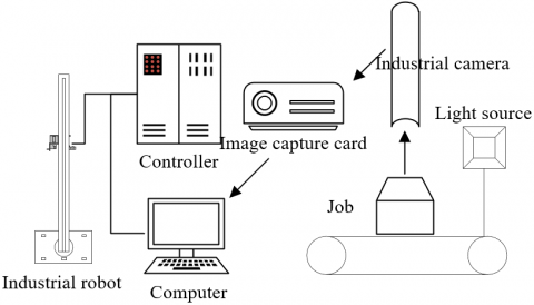
Figure 5. Structure of job recognition and sorting system
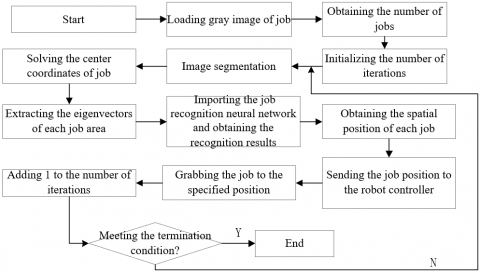
Figure 6. Flow chart of job sorting
This paper builds a fast job recognition and smart sorting system based on industrial camera, industrial robot and its controller, computer, and image capture card. The system structure is described in Figure 5. The system operates in the following procedure: First, each target job is placed on the workbench. Then, the industrial camera captures images on the job. The images are transmitted to the computer for processing. The recognition result and job position will be uploaded to the upper computer. Then, the image processing software of the visual system will process and recognize all the jobs in the received image. Through image segmentation and shape feature extraction of job areas, the job classes and spatial positions will be obtained. The results will be reported to the industrial robot. Next, the controller will automatically plan the path for job sorting, and then drive the robot to sort all the jobs. The job sorting process is explained in Figure 6.
Industrial sorting raises strict requirements on the accuracy of job classification, positioning, counting, capturing, and placement. Traditional robot sorting cannot effectively adapt to complex production environments. By contrast, robot sorting, coupled with MV and image processing, can greatly improve production efficiency, making the sorting more flexible and smarter. The key of smart job sorting lies in the creation of an ideal MV system, the design of an accurate job feature extraction algorithm, and a good neural network for job class recognition. After the job edge features have been extracted, the sorting procedure can be described as follows:
Step 1. Compute the total number of jobs based on the connected domains in the image.
Step 2. Set the cycle for completely sorting one job (the cyclic procedure will be terminated after all jobs have been sorted).
Step 3. Solve the center coordinates of each job, and obtain the eigenvector of its edge. Import all information to the neural network for job recognition, and obtain the spatial position of the job under the robot coordinate system through coordinate system transform.
Step 4. Start grabbing the job after the controller determines the job position.
Step 5. Repeat Steps 2-4 until all sorting tasks are complete.
Tables 1 and 2 show the wavelet moment features and wavelet descriptor features corresponding to different jobs, respectively. There are mainly eight kinds of jobs in our experiments: faceplate, pull rod, support, latch, sliding block, sealed cap latch, blade holder, and motor seat. After setting the scale factor and translation factor, the frequency components of wavelet features Q0,0,0~Q1,1,0 in the phase space [0, 180°] were given under different NS and MT. Then, the wavelet moment features can be extracted from different types of job images by computing the mean inter-class distance of each class:
$\zeta_{i, j}=\frac{\left|Q_{i}^{\prime}-Q_{j}^{\prime}\right|}{\sqrt{v_{i}^{2}+v_{j}^{2}}}$ (31)
where, Q'I and Q'j are the mean wavelet moment features of job images of the i-th and j-th classes, respectively; υ2i and υ2j are the feature variances of job images of the i-th and j-th classes, respectively. Similarly, the mean error and error variance of each class of job images were calculated by formula (17), thereby discarding the unqualified wavelet descriptor features.
To verify if the job matching method is accurate enough for job sorting, the job center coordinates under the actual working condition of 4mm with the actual job center coordinates. Table 3 presents the job template matching results under different rules. It can be seen that the center coordinates extracted under 8 rules are all successful, indicating the feasibility of our job template matching method.
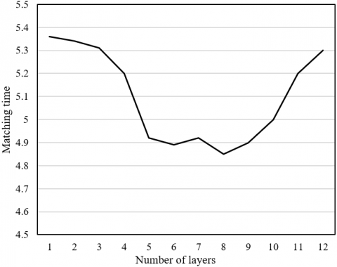
Furthermore, the pyramid search model of the proposed job template matching approach was verified on the MV software HALCON. Figure 7 records how the matching time varies with the changing number of pyramid layers, under the minimum threshold of 0.7. As the pyramid layers changed from 1 to 12, the jobs were always successfully matched, but with different time consumptions. The matching time was relatively short when the pyramid had 5 to 9 layers. Hence, [5, 9] was selected as the optimal number of pyramid layers.
Table 1. Wavelet moment features of different jobs
|
|
1 |
2 |
3 |
4 |
5 |
6 |
7 |
8 |
|
Q0,0,0 |
6.542 |
8.326 |
3.208 |
2.456 |
6.153 |
3.182 |
7.345 |
8.137 |
|
Q0,1,0 |
5.786 |
8.456 |
3.582 |
2.053 |
6.049 |
2.895 |
7.964 |
8.876 |
|
Q1,1,0 |
6.057 |
7.786 |
3.786 |
2.571 |
6.186 |
3.543 |
7.122 |
8.012 |
|
Q1,0,0 |
5.123 |
7.164 |
3.547 |
2.784 |
6.376 |
3.785 |
7.749 |
8.961 |
Table 2. Wavelet descriptor features of different jobs
|
|
1 |
2 |
3 |
4 |
5 |
6 |
7 |
8 |
|
J10 |
4.293 |
3.453 |
0.687 |
4.438 |
10.456 |
9.315 |
7.251 |
4.157 |
|
J20 |
4.768 |
4.210 |
0.658 |
4.675 |
10.378 |
10.452 |
7.912 |
4.215 |
|
J30 |
4.123 |
3.078 |
0.613 |
4.215 |
10.791 |
9.044 |
7.264 |
4.346 |
Table 3. Template matching results of jobs under different rules
|
Job type |
Job center coordinates extracted through template matching |
Corresponding coordinates under robot coordinate system |
Actual job center coordinates |
Spacing |
Matching result |
|
Faceplate |
(145.21,253.33) |
(385,451) |
(387,452) |
2.13 |
Successful |
|
Pull rod |
(147.81,511.46) |
(351,618) |
(352,621) |
1.35 |
Successful |
|
Support |
(163.38,672.53) |
(382,742) |
(389,745) |
2.22 |
Successful |
|
Latch |
(372.75,652.72) |
(749,673) |
(752,683) |
2.37 |
Successful |
|
Sliding block |
(259.37,542.38) |
(376,409) |
(379,412) |
2.19 |
Successful |
|
Seal cap latch |
(268.59,395.14) |
(359,715) |
(361,717) |
2.45 |
Successful |
|
Blade holder |
(395.25,276.27) |
(713,684) |
(718,685) |
2.34 |
Successful |
|
Motor seat |
(298.13,275.92) |
(343,626) |
(342,621) |
2.28 |
Successful |
Figure 7. Matching time variation with the changing number of pyramid layers
Figure 8. Matching time variation with the changing minimum threshold
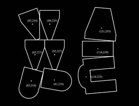
Figure 8 shows how the matching time varies, as the minimum threshold changes from 0.1 to 1, while the pyramid layers remain the same. During the optimization, the matching time changed with a steeper slope as the minimum threshold increased in [0.1, 0.8] than that as the minimum threshold changed in [0.8, 1]. The former scenario had greater impact on the matching time than the latter. Figure 9 presents the edges of the extracted jobs; Figure 10 displays the recognition results of adjoining jobs.
Table 4 summarizes the experimental results of the proposed job recognition method. The results show that the variation of the job types and positions on the workbench did not affect the job recognition and positioning accuracy of our system, whose accuracy remained at 100%. Hence, our method is highly feasible for job sorting in actual working conditions.
After repeated sorting experiments, the time consumed by each module of our system was recorded (Table 5). From image shooting to the end of image processing, the time consumption stood at 1.42s; from the start of job matching to the output of recognition results and position information, the time consumption was 0.35s; from the controller receiving the position signal to the robot completing job sorting, the time consumption was 2.1s. Overall, our system achieved good stability and real-time performance, recognized and sorted the jobs quickly, and adapted well to different working conditions.
Figure 9. Edges of the extracted jobs
Figure 10. Recognition results on adjoining jobs
Table 4. Experimental results of the proposed job recognition method
|
Serial number |
Number of jobs |
Corresponding coordinates under robot coordinate system |
Actual job center coordinates |
Spacing |
Matching result |
|
1 |
7 |
(105,98) |
(106,101) |
2.21 |
Successful |
|
2 |
5 |
(241,229) |
(243,232) |
2.35 |
Successful |
|
3 |
2 |
(375,379) |
(376,383) |
2.27 |
Successful |
|
4 |
4 |
(187,192) |
(182,189) |
2.16 |
Successful |
|
5 |
3 |
(179,181) |
(178,185) |
1.42 |
Successful |
|
6 |
8 |
(352,356) |
(347,351) |
2.34 |
Successful |
|
7 |
6 |
(275,278) |
(273,272) |
2.18 |
Successful |
|
8 |
6 |
(156,162) |
(159,168) |
1.52 |
Successful |
|
9 |
2 |
(198,203) |
(192,204) |
1.75 |
Successful |
|
10 |
5 |
(321,325) |
(323,327) |
1.98 |
Successful |
Table 5. Time consumption of each module
|
Module name |
Image preprocessing |
Job recognition |
Positioning |
Total |
|
Time |
1.4253 |
0.3521 |
0.0257 |
1.735 |
Based on image processing, this paper proposes a fast job recognition and sorting method. After detailing the extraction approach for wavelet moment features and wavelet descriptors, the authors described the feature fusion process based on the ESN, introduced the idea of job template matching, and discussed how to measure similarity and terminate the measurement during template matching. After that, the features of wavelet moments and descriptors of different jobs were calculated, and used to derive the principles of discarding and retaining these features. Moreover, the job template matching was carried out under different rules, and the matching time variations with pyramid layers and minimum threshold were observed, which together demonstrate the effectiveness of our job template matching strategy. Furthermore, the extracted job edges and recognition results of adjoining jobs were given, suggesting that our algorithm is accurate enough in job recognition. Finally, the time consumption of each module was recorded, which indicates that our sorting system has good stability and real-time performance.
[1] Dong, R.G., Welcome, D.E., Xu, X.S., McDowell, T.W. (2020). Identification of effective engineering methods for controlling handheld workpiece vibration in grinding processes. International Journal of Industrial Ergonomics, 77: 102946. https://doi.org/10.1016/j.ergon.2020.102946
[2] Wang, L., Liu, J., Ye, Q., Cheng, H., Zhi, J. (2020). Sorting method of lithium-ion batteriesinmass production. IOP Conference Series: Earth and Environmental Science, 512(1): 012127. https://doi.org/10.1088/1755-1315/512/1/012127
[3] Li, A.D., He, Z. (2020). Multiobjective feature selection for key quality characteristic identification in production processes using a nondominated-sorting-based whale optimization algorithm. Computers & Industrial Engineering, 149: 106852. https://doi.org/10.1016/j.cie.2020.106852
[4] Chen, X., An, Y., Zhang, Z., Li, Y. (2020). An approximate nondominated sorting genetic algorithm to integrate optimization of production scheduling and accurate maintenance based on reliability intervals. Journal of Manufacturing Systems, 54: 227-241. https://doi.org/10.1016/j.jmsy.2019.12.004
[5] Overby, E., Mitra, S. (2014). Physical and electronic wholesale markets: An empirical analysis of product sorting and market function. Journal of Management Information Systems, 31(2): 11-46. https://doi.org/10.2753/MIS0742-1222310202
[6] Singh, D., Yousefi, R., Boroushaki, M. (2011). Identification of optimum parameters of deep drawing of a cylindrical workpiece using neural network and genetic algorithm. World Academy of Science, Engineering and Technology, 78: 211-217. https://doi.org/10.5281/zenodo.1056334
[7] Denkena, B., Bergmann, B., Witt, M. (2019). Material identification based on machine-learning algorithms for hybrid workpieces during cylindrical operations. Journal of Intelligent Manufacturing, 30(6): 2449-2456. https://doi.org/10.1007/s10845-018-1404-0
[8] Zemzemi, F., Rech, J., Salem, W.B., Dogui, A., Kapsa, P. (2009). Identification of a friction model at tool/chip/workpiece interfaces in dry machining of AISI4142 treated steels. Journal of Materials Processing Technology, 209(8): 3978-3990. https://doi.org/10.1016/j.jmatprotec.2008.09.019
[9] Liu, C., Xiang, S., Lu, C., Wu, C., Du, Z., Yang, J. (2020). Dynamic and static error identification and separation method for three-axis CNC machine tools based on feature workpiece cutting. The International Journal of Advanced Manufacturing Technology, 107: 2227-2238. https://doi.org/10.1007/s00170-020-05103-5
[10] Tung, P.D. (2018). Mathematical modeling and parametric identification of dynamic properties of mechanical subsystems tool and workpiece in turning process. In MATEC Web of Conferences, 226: 02017. https://doi.org/10.1051/matecconf/201822602017
[11] Wang, X., Atungulu, G.G., Gebreil, R., Gao, Z., Pan, Z., Wilson, S.A., Olatunde, G., Slaughter, D. (2017). Sorting in-shell walnuts using near infrared spectroscopy for improved drying efficiency and product quality. International Agricultural Engineering Journal, 26(1): 165-172.
[12] Kruethi, N., Chaijit, S., Permpoonsinsup, W., Thongkot, D., Ismail, A.H., Srinoi, P. (2019). Simulation modelling for productivity improvement of sorting process in a ceramic plant. 2019 17th International Conference on ICT and Knowledge Engineering (ICT&KE), Bangkok, Thailand, pp. 1-4. https://doi.org/10.1109/ICTKE47035.2019.8966820
[13] Pfeisinger, C. (2017). Material recycling of post-consumer polyolefin bulk plastics: Influences on waste sorting and treatment processes in consideration of product qualities achievable. Waste Management & Research, 35(2): 141-146. https://doi.org/10.1177/0734242X16669998
[14] Mashhadi, A.R., Behdad, S. (2017). Optimal sorting policies in remanufacturing systems: Application of product life-cycle data in quality grading and end-of-use recovery. Journal of Manufacturing Systems, 43: 15-24. https://doi.org/10.1016/j.jmsy.2017.02.006
[15] Ali, M.S.R., Pal, A.R. (2017). Multi machine operation with product sorting and elimination of defective product along with packaging by their colour and dimension with speed control of motors. 2017 International Conference on Electrical, Electronics, Communication, Computer, and Optimization Techniques (ICEECCOT), Mysuru, India, pp. 1-6. https://doi.org/10.1109/ICEECCOT.2017.8284575
[16] Ali, M.S., Ali, M.S.R. (2017). Automatic multi machine operation with product sorting and packaging by their colour and dimension with speed control of motors. In 2017 international conference on advances in electrical technology for green energy (ICAETGT), Coimbatore, India, pp. 88-92. https://doi.org/10.1109/ICAETGT.2017.8341466
[17] Kothuru, A., Nooka, S.P., Iglesias Victoria, P., Liu, R. (2017). Application of audible sound signals for tool wear monitoring and workpiece hardness identification in gear milling using machine learning techniques. International Design Engineering Technical Conferences and Computers and Information in Engineering Conference, 58240: V010T11A030. https://doi.org/10.1115/DETC2017-68067
[18] Otko, T., Zębala, W. (2016). Identification and analysis of residual stresses in the axisymmetric workpiece existing before and after machining. Key Engineering Materials, 686: 33-38. https://doi.org/10.4028/www.scientific.net/KEM.686.33
[19] Abdelali, H.B., Courbon, C., Rech, J., Ben Salem, W., Dogui, A., Kapsa, P. (2011). Identification of a friction model at the tool-chip-workpiece interface in dry machining of a AISI 1045 steel with a TiN coated carbide tool. Journal of Tribology, 133(4): 042201. https://doi.org/10.1115/1.4004879
[20] Segurajauregui, U., Arrazola, P.J. (2015). Heat-flow determination through inverse identification in drilling of aluminium workpieces with MQL. Production Engineering, 9(4): 517-526. https://doi.org/10.1007/s11740-015-0631-x
[21] Schindler, S., Zimmermann, M., Aurich, J.C., Steinmann, P. (2015). Identification of thermal effects on the diameter deviation of inhomogeneous aluminum metal matrix composite workpieces when dry turning. Production Engineering, 9(4): 473-485. https://doi.org/10.1007/s11740-015-0629-4
[22] Eswari, J.S., Venkateswarlu, C. (2020). Multiobjective Pareto optimisation of pharmaceutical product formulation using radial basis function network and non-dominated sorting differential evolution. International Journal of Biomedical Engineering and Technology, 33(2): 95-122. https://doi.org/10.1504/IJBET.2020.107707
[23] Wahdan, H., Abdelslam, H., Abou-El-Enien, T., Kassem, S. (2019). Sustainable product design through non-dominated sorting cuckoo search. Journal Européen des Systèmes Automatisés, 52(5): 439-448. https://doi.org/10.18280/jesa.520502
[24] Gutt, D. (2018). Sorting Out the Lemons–Identifying Product Failures in Online Reviews and their Relationship with Sales. Proceedings of the Multikonferenz Wirtschaftsinformatik (MKWI), Lüneburg, Germany, pp. 1649-1655.
[25] Nishiyama, M., Sato, R., Shirase, K. (2012). 3D model construction of cutting tools and identification of workpieces using machine vision for virtual machining simulation. International Symposium on Flexible Automation, 45110: 43-46. https://doi.org/10.1115/ISFA2012-7204
[26] Tsai, H.H., Hocheng, H. (2002). On-line identification of thermally-induced convex deformation of the workpiece in surface grinding. Journal of Materials Processing Technology, 121(2-3): 189-201. https://doi.org/10.1016/S0924-0136(01)01058-5
[27] Labbi, O., Ahmadi, A., Ouzizi, L., Douimi, M. (2020). A non-dominant sorting genetic algorithm for optimization of a product design and selection of its suppliers. Journal of Advanced Manufacturing Systems, 19(1): 167-188. https://doi.org/10.1142/S0219686720500092