Fuchun Jiang* | Hongyi Zhang | Chen Zhu
© 2021 IIETA. This article is published by IIETA and is licensed under the CC BY 4.0 license (http://creativecommons.org/licenses/by/4.0/).
OPEN ACCESS
The current three-dimensional (3D) target detection model has a low accuracy, because the surface information of the target can only be partially represented by its two-dimensional (2D) image detector. To solve the problem, this paper studies the 3D target detection in the RGB-D data of indoor scenes, and modifies the frustum PointNet (F-PointNet), a model superior in point cloud data processing, to detect indoor targets like sofa, chair, and bed. The 2D image detector of F-PointNet was replaced with you only look once (YOLO) v3 and faster region-based convolutional neural network (R-CNN) respectively. Then, the F-PointNet models with the two 2D image detectors were compared on SUN RGB-D dataset. The results show that the model with YOLO v3 did better in target detection, with a clear advantage in mean average precision (>6.27).
indoor RGB-D data, target detection, detection accuracy, frustum PointNet (F-PointNet)
With the recent development of deep learning (DL), image processing technologies have emerged one after another, bringing considerable achievements in image-based target detection. However, not many scholars have applied DL to target detection of three-dimensional (3D) point cloud data. Compared with two-dimensional (2D) images, 3D point cloud data can accurately represent the surface information, [1] and some depth information [2] of the target. Because of its various sources, 3D point cloud data have attracted a growing attention, making it interesting to further apply DL to target detection of 3D point cloud data.
Currently, it is an open question how could 3D point cloud data be imported to neural networks by DL. To facilitate the importation, the literature [3] adopted the energy equation to obtain the 3D regression frame under the framework of the fast region-based convolutional neural network (R-CNN). However, there is yet no practical or effective detection method for occluded target. Under the architecture of faster R-CNN, Literature [4] proposed a 3D region proposal network (RPN), which can effectively detect occluded targets. But the 3D RPN is too slow to achieve real-time processing. Under the framework of you only look once (YOLO) network, Literature [5] drew the merits of relevant research [6-8], and came up with a new CNN architecture. With a running rate of 50 frames per second (fps), the new architecture reaches the standard for real-time processing. Nonetheless, the architecture has errors in the conversion between 3D and 2D coordinates, resulting in large detection errors on small targets. Literature [9] proposed the DenseFusion network, which covers the depth information of each pixel in the image. The network greatly improves the real-time processing speed, but does not perform well in small target detection. Literature [10-12] converted point cloud data into image information, and detected targets with fusion and projection techniques [13-15]. However, the above approaches are defected in target detection, because they more or less ignore the disordered and local correlations in point cloud data.
This paper adopts the frustum PointNet (F-PointNet) [16] model to directly process the original point cloud data, and realize target detection of 3D point cloud data, without needing to convert the input data into point cloud data. Considering the restrictions on the features of point cloud data, this strategy does not generate an overlarge dataset after data conversion, avoids unnecessary calculations, improves resource utilization, and ensures better detection effect.
The F-PointNet generates a 2D area proposal from the original image, locates it in the 3D point cloud data, and thereby extracts the corresponding point cloud data. Then, the point clou data are processed by the segmentation network of PointNet [17], and 3D bounding box evaluation for 3D target detection.
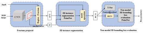
The basic architecture of F-PointNet (Figure 1) contains three modules: the frustum proposal module, the 3D instance segmentation module, and the non-modal 3D bounding box evaluation module.
2.1 Frustum proposal module
In this module, 2D image target detection technology is employed to classify the corresponding target in the image, extract the target area, and obtain the parameters of the 2D bounding box of the target. Then, the 2D target area is extracted and mapped to the 3D point cloud data, based on the depth information of the RGB-D image and the camera projection matrix. From the 3D point cloud data, the frustum containing the target is extracted. The specific procedure is summarized as follows:
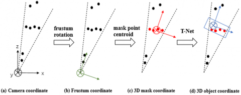
First, read the coordinates, images and labels of 3D point cloud, and the data on the related conversion matrix from the SUN RGB-D dataset [18-21]. Next, map the 2D bounding box to the 3D point cloud through the conversion matrix, and filter out the point clouds outside the corresponding area in the 2D plane. After that, implement a series of coordinate conversions (Figure 2) and point cloud extractions/processing to extract the frustum 3D point cloud data corresponding to the target area.
Figure 1. Basic structure of F-PointNet model
Note: n is the number of point clouds of the frustum point cloud extracted by frustum proposal module; m is the number of point clouds of the target point cloud after instance segmentation; c is the number of point cloud channels; k is the number of target classes in point cloud.
Each extracted frustum point cloud has a unique direction in the camera coordinate system. To facilitate data processing, it is necessary to convert the coordinate system of the frustum point cloud data from the camera coordinate system to the frustum coordinate system. As shown in Figure 2, the centerline of the frustum point cloud is rotated to a position orthogonal to the image plane; then, the point cloud coordinates are converted to the frustum coordinate system.
Figure 2. Point cloud coordinates
2.2 3D instance segmentation module
As its name suggests, this module mainly semantically segments the point cloud. As shown in Figure 3, the module receives the point cloud data extracted by the previous module, implements semantic segmentation of the frustum point cloud data with the aid of the one-hot vector, which is generated through frustum extraction, and outputs the score of the class of the 3D point cloud. The output score is a binary score for the detection of target point cloud and other non-target point clouds (background point clouds or other messy point clouds). In this module, the mask operation combines the scores of semantic segmentation, removes non-target point clouds from the input 3D point cloud data of the frustum, and extracts the point cloud of the target instance. After that, the coordinates of the extracted target point cloud are converted from the frustum coordinate system (Figure 2(b)) to the mask coordinate system (Figure 2(c)), with the centroid of the target point cloud as the origin. During the conversion, the centroid coordinates of the target point cloud need to be subtracted from all the target point clouds, forming the point cloud data in the mask coordinate system.
Figure 3. Structure of 3D instance segmentation module
Note: n is the number of point clouds in the frustum point cloud; k is the number of target classes; mlp is multi-layer perceptron.
2.3 Non-modal 3D bounding box evaluation module
This module predicts the 3D bounding box of the target in the 3D point cloud, based on the target point cloud data in the mask coordinate system. The target centroid in the mask coordinate system obtained by the previous module is not the centroid of the real target. This is because, when the Velodyne Lidar sensor scans the target, the point cloud obtained is merely part of the point cloud data of the target facing the radar direction. Therefore, the centroid position is adjusted with the help of a lightweight T-Net (Figure 4), combined with the global vector generated by the one-hot vector. The residual data related to the centroid adjustment are generated by the fully-connected layers. After that, the residual data are subtracted from all the point cloud data, producing the point cloud data in the local coordinate system (Figure 2(d)), with the real target centroid as the origin.
After moving the target centroid and target point cloud through T-Net, all point clouds are converted to the predicted real target centroid as the origin of the local coordinate system, and then processed by the non-modal 3D bounding box evaluation module (Figure 5). After being processed by an MLP similar to T-Net, the FCs eventually output all the parameter information evaluated by the module, including the centroid coordinates, length, width, and height of the bounding box, residual error, heading angle, etc.
Figure 4. T-Net structure
Note: FCs are fully-connected layers; the numbers behind FCs are the number of output channels in each FC.
Figure 5. Structure of non-modal 3D bounding box evaluation module
2.4 Loss function
In the entire model, multiple networks are adopted to train the 3D point cloud data, including the 3D instance segmentation PointNet network of the 3D instance segmentation module, and the T-Net and the PointNet network in the non-modal 3D bounding box evaluation module. The training losses of these networks are integrated into the loss L of the overall model:
$\begin{array}{c}
L=L_{s e g}+\lambda\left(L_{c 1-r e g}+L_{c 2-r e g}+L_{h-c l s}+L_{h-r e g}\right. \\
\left.+L_{s-c l s}+L_{s-r e g}+\gamma L_{\text {corner }}\right)
\end{array}$ (1)
where, Lseg is the semantic segmentation loss in the 3D instance segmentation of the PointNet; Lc1-reg is the centroid conversion loss generated by the T-Net; Lc2-reg is the non-modal centroid conversion loss of the 3D bounding box evaluation PointNet; Lh-cls and Lh-reg are the classification loss and semantic segmentation loss of heading angle of the network model, respectively; Ls-cls and Ls-reg are the classification and semantic segmentation losses of the bounding box size of the network predicting the 3D bounding box, respectively; λ=1 and γ=10 are model parameters; Lcorner is the total loss of the eight predicted corners of the 3D bounding box:
$L_{\text {corner }}=L_{\delta}\left(\sum _ { i = 1 } ^ { 8 } \sum _ { j = 1 } ^ { 1 2 } \operatorname { m i n } \left\{\sum_{k=1}^{8}\left\|P_{k}^{\mathrm{ij}}-\mathrm{P}_{k}^{*}\right\|, \sum_{\mathrm{k}=1}^{8} \| \mathrm{P}_{\mathrm{k}}^{\mathrm{ij}}\right.\right.$$\left.\left.-\mathrm{P}_{\mathrm{k}}^{* *} \|,\right\}\right)$ (2)
where, $P_{k}^{i j}$ is the 3D vector of the k-th corner of the anchor box; i is the number of the bounding boxes of eight sizes in the anchor box; j is the number of the bounding boxes with twelve heading angles in the anchor box; k is the number of the middle corners of the 8 corners of the bounding box; $P_{k}^{*}$ is the 3D vector of the k-th corner of the real 3D bounding box; $\left\|P_{k}^{i j}-P_{k}^{*}\right\|$ is the distance between the k-th corner of the 3D anchor box and the k-th corner of the real 3D bounding box; $P_{k}^{* *}$ is the 3D vector of the k-th corner of the 3D real bounding box after being flipped by the angle π (the distance between the predicted angle vector and the flipped vector needs to be calculated, because the dataset is enhanced by flipping in the experiment); $\left\|P_{k}^{i j}-P_{k}^{* *}\right\|$ is the distance between the k-th corner of the 3D anchor box and the k-th corner of the flipped bounding box; $L_{\delta}(a)$ is the Huber loss function:
$L_{\delta}(a)=\left\{\begin{array}{c}
\frac{1}{2} a^{2},|a| \leq \delta \\
\delta\left(|a|-\frac{1}{2} \delta\right), \text { otherwise }
\end{array}\right.$ (3)
where, a is the input of Huber loss function; $\delta$ is the control parameter of the angle loss of the entire network. In the Huber loss function, the angle loss is fitted from square error and linear error. Before predicting the 3D bounding box of the target point cloud, the authors predesigned eight anchor boxes with different lengths, widths and heights, and 12 anchor boxes with different heading angles, plus the boundaries between adjacent boxes. The heading angle difference between the boxes is 30°, and each anchor box contains 8 corners.
3.1 2D image detector
In 3D target detection, it is critical to choose a suitable algorithm for the 3D image detector. This paper selects YOLOv3 and faster R-CNN as the algorithms for 2D image detector. The former has delivered ideal experimental results on the SUN RGB-D dataset, as a 2D image detector.
3.2 Parameter initialization
Parameter initialization is an important step in neural network application. The main parameters to be initialized in our work are weights and bias. During network training, the bias is set to zero, but not all weights are initialized as zero. Otherwise, the network will have the same weights during model training, which will dampen the detection result. Therefore, two strategies were selected for parameter initialization: the Xavier method and the truncated normal distribution method. The Xavier method keeps the activation value of each layer consistent with the variance of the output, and ensures the uniform distribution of the generated parameters. The truncated normal distribution method guarantees the normal distribution of the initial values, and controls the difference between and average of all generated values below twice the standard deviation after taking the absolute value.
Figure 6 shows the test results on target detection accuracies of the two different initialization methods. It can be seen that the Xavier method achieved faster convergence, better detection effect, and high efficiency than truncated normal distribution method.
Figure 6. Target detection accuracies of different initialization methods
3.3 γ2 regularization
During model training on massive data, it is crucial to avoid overfitting and enhance the generalization ability of the model. Thus, a $\gamma 2$ regularization term was added to the original loss function:
$C=C_{0}+\frac{\delta}{2 n} \sum \omega^{2}$
where, C is the total loss of C0 after adding the weight attenuation term; C0 is the loss before adding γ2 regularization; $\frac{\delta}{2 n} \sum \omega^{2}$ is the loss term after γ2 regularization; ω is the weight in the neural network; δ is the γ2 regularization coefficient; n is the number of training samples.
The reduction of network loss drags down the weight of the network, making the network less complex and better performing in data fitting. The loss function after $\gamma 2$ regularization can be defined as:
$\left\{\begin{array}{c}
L=L_{s e g} \\
+\lambda\left(\begin{array}{c}
L_{c 1-r e g}+L_{c 2-r e g}+L_{h-c l s}+L_{h-r e g} \\
+L_{s-c l s}+L_{s-r e g}+\gamma L_{\text {corner }}
\end{array}\right)+C \\
C=C_{0}+\frac{\delta}{2 n} \sum \omega^{2}
\end{array}\right.$
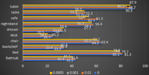
Figure 7 shows the test results on target detection accuracies of different regularization coefficients. It can be seen that, when the weight attenuation term was zero, the highest detection accuracies were achieved on chair, desk, nightstand, and toilet; when the regularization coefficient was 0.01, the highest detection accuracies were achieved on bathtub, bed, bookshelf, and sofa; when the coefficient was 0.0005, the highest detection accuracy was achieved on dresser.
Figure 7. Target detection accuracies of different regularization coefficients
Overall, the best weight attenuation term should be set to 0.01. Under this setting, the detection accuracies of chair, desk, nightstand, and toilet are slightly lower than the no-weight scenario, but those of bathtub, bed, bookshelf, and sofa are significantly improved.
3.4 Dataset
Most previous 3D detection studies focus on outdoor lidar scanning. The targets are well separated in space, and the point cloud has sparse (feasible for bird’s-eye projection), or dense pixels. The CNN can be easily applied on the indoor depth map of conventional images. However, a method designed for bird’s-eye view may not be possible for indoor environment, where multiple targets often throng in the same vertical space. Moreover, the large and sparse point clouds scanned by lidar may be difficult to apply to indoor focusing techniques. Fortunately, the F-PointNet is a general detection framework for outdoor and indoor 3D targets [22]. The network can achieve ideal performance was achieved on SUN RGB-D database [18], with a high mean average precision (mAP) and fast inference speed.
4.1 DL configuration
The improved -PointNet detection algorithm was implemented under the DL framework TensorFlow. The server platform was configured as follows: Intel ® CoreTM i7-7700K CPU@4.2GHz processor, 16GB memory, 1T hard disk, 8GB GeForce GTX 1080 GPU.
4.2 Parameter analysis
The model structure (Figure 1) is mainly composed of 3D instance segmentation network (Figure 3), T-Net (Figure 4), and non-modal 3D bounding box evaluation network (Figure 5) [23]. The first network contains ten convolutional layers; the T-Net consists of several convolutional layers (the kernel outputs are 128, 128, and 256 pixels in size) and three FCs (in the MLP (128, 128, 256) layer); the third network involves 4 convolutional layers and 3 FCs. The SUN RGB-D dataset was adopted for our experiments. There are 7,481 images and 748 3D point cloud data files in the dataset. The dataset was divided by the Multi-View 3D networks (MV3D) method into a training set of 3,712 files and a test set of 3,769 files. The batch size was set to 32, i.e., each batch contains 32 point cloud data files as the network input [24].
In addition, the network training lasts 200 iterations, with the initial learning rate of 0.0001. To stabilize the network performance, the exponential decay method was adopted to reduce the learning rate by half for every 25,000 batches. The learning rate was kept constant after reaching 0.0001.
4.3 Comparison of target detection accuracies
The 2D image detector in F-PointNet was modified by YOLOv3 and faster R-CNN, respectively. Table 1 compares the detection accuracies of 3D point cloud data targets between the two modified methods. Obviously, the YOLOv3 model achieved higher accuracies on bed, bookshelf, chair, dresser, nightstand, sofa, table, and toilet than the faster R-CNN model, and slightly lower accuracies on bathtub and desk [25, 26].
Table 1. Comparison between YOLOv3 and faster R-CNN
|
2D image detector |
Faster R-CNN |
YOLOv3 |
|
Bathtub |
58.0 |
43.6 |
|
Bed |
63.1 |
81.6 |
|
Bookshelf |
32.8 |
33.4 |
|
Chair |
62.2 |
64.4 |
|
Desk |
45.9 |
25.1 |
|
Dresser |
15.7 |
32.1 |
|
Nightstand |
27.1 |
57.5 |
|
Sofa |
51.8 |
61.6 |
|
Table |
51.4 |
51.3 |
|
Toilet |
70.6 |
90.7 |
|
Mean |
47.86 |
54.13 |
Table 2. Comparison between different detection methods
|
Methods |
DSS [19] |
COG [20] |
2D-driven method [21] |
F-PointNet [16] |
Our method |
|
Bathtub |
44.2 |
58.3 |
43.5 |
43.3 |
43.6 |
|
Bed |
78.8 |
63.7 |
64.5 |
81.1 |
81.6 |
|
Bookshelf |
11.9 |
31.8 |
31.4 |
33.3 |
33.4 |
|
Chair |
61.2 |
62.2 |
48.3 |
64.2 |
64.4 |
|
Desk |
20.5 |
45.2 |
27.9 |
24.7 |
25.1 |
|
Dresser |
6.4 |
15.5 |
25.9 |
32.0 |
32.1 |
|
Nightstand |
15.4 |
27.4 |
41.9 |
58.1 |
57.5 |
|
Sofa |
53.5 |
51.0 |
50.4 |
61.1 |
61.6 |
|
Table |
50.3 |
51.3 |
37.0 |
51.1 |
51.3 |
|
Toilet |
78.9 |
70.1 |
80.4 |
90.9 |
90.7 |
|
Runtime |
19.55s |
10-30min |
4.15s |
0.12s |
1.42s |
|
mAP |
42.1 |
47.6 |
45.1 |
54.0 |
54.13 |
Further, the 2D image detector in F-PointNet was replaced with YOLOv3, and the modified model was compared with the original F-PointNet, deep sliding shape (DSS) network [27], clouds of oriented gradients (COG) [28], and 2D-driven method [4]. Table 2 presents the detection accuracies of these methods on 3D point cloud data targets. It can be seen that our model was more accurate on bathtub, bed, bookshelf, chain, desk, dresser, sofa, and table than the other methods, and was only slightly less accurate than the original F-PointNet on nightstand. Hence, the modification of the 2D image detector indeed improves the generalization ability of the model.
4.4 Visualization of detection results
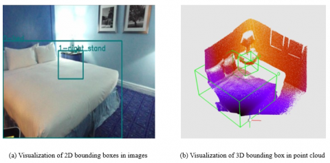
The detection results of the modified F-PointNet model were visualized according to the 3D bounding box parameters outputted by the model. Figure 8 shows an image and the visualized point cloud data. In the image taken by the camera, the target area is marked by a 2D blue bounding box. The visualized data were zoomed in to clearly display the predicted 3D bounding box.
Figure 8. Image and point cloud visualization
This paper modifies the F-PointNet for the target detection of 3D point cloud data. The 2D image detector of the original network was changed into YOLOv3, and the test dataset was replaced with SUN RGB-D room. Experimental results show that the modified model can effectively detect targets of 3D point cloud data [28]. Therefore, the modified F-PointNet model is suitable for indoor robot navigation and many other fields.
Of course, our model also has some shortcomings: (1) The detection results are greatly affected by target detection in 2D images. If the targets are severely occluded or dim, it is difficult to determine the 2D bounding boxes. (2) The 3D bounding box might be inaccurate, if the target point cloud is small [4]. To make our model more applicable to real scenes, the future research will try to make up for the defects with high-resolution images.
[1] Xue, R. (2017). Point cloud registration based on RGB-D data. Chang'an University, Xi'an, China.
[2] Zhao, X. (2010). Research on 3D reconstruction method based on surface laser scanning point cloud data. Wuhan University, Wuhan, China.
[3] Chen, X., Kundu, K., Zhu, Y., Berneshawi, A.G., Ma, H., Fidler, S., Urtasun, R. (2015). 3d object proposals for accurate object class detection. In Advances in Neural Information Processing Systems, 424-432. https://doi.org/10.1.1.705.5656
[4] Song, S., Xiao, J. (2016). Deep sliding shapes for amodal 3d object detection in RGB-d images. In Proceedings of the IEEE Conference on Computer Vision and Pattern Recognition, 808-816.
[5] Tekin, B., Sinha, S.N., Fua, P. (2018). Real-time seamless single shot 6d object pose prediction. In Proceedings of the IEEE Conference on Computer Vision and Pattern Recognition, pp. 292-301.
[6] Dhiman, V., Tran, Q.H., Corso, J.J., Chandraker, M. (2016). A continuous occlusion model for road scene understanding. In Proceedings of the IEEE Conference on Computer Vision and Pattern Recognition, pp. 4331-4339.
[7] Redmon, J., Farhadi, A. (2017). YOLO9000: Better, faster, stronger. In Proceedings of the IEEE Conference on Computer Vision and Pattern Recognition, pp. 7263-7271.
[8] Long, J., Shelhamer, E., Darrell, T. (2015). Fully convolutional networks for semantic segmentation. In Proceedings of the IEEE Conference on Computer Vision and Pattern Recognition, pp. 3431-3440.
[9] Wang, C., Xu, D., Zhu, Y., Martín-Martín, R., Lu, C., Li, F.F., Savarese, S. (2019). DenseFusion: 6D object pose estimation by iterative dense fusion. In Proceedings of the IEEE/CVF Conference on Computer Vision and Pattern Recognition, pp. 3343-3352.
[10] Ren, S., He, K., Girshick, R., Sun, J. (2015). Faster r-CNN: Towards real-time object detection with region proposal networks. arXiv preprint arXiv:1506.01497.
[11] Su, H., Maji, S., Kalogerakis, E., Learned-Miller, E. (2015). Multi-view convolutional neural networks for 3d shape recognition. In Proceedings of the IEEE International Conference on Computer Vision, pp. 945-953.
[12] Li, B., Zhang, T., Xia, T. (2016). Vehicle detection from 3d lidar using fully convolutional network. arXiv preprint arXiv:1608.07916.
[13] Hirschmuller, H. (2007). Stereo processing by semiglobal matching and mutual information. IEEE Transactions on Pattern Analysis and Machine Intelligence, 30(2): 328-341. https://doi.org/10.1109/TPAMI.2007.1166
[14] Chen, X., Ma, H., Wan, J., Li, B., Xia, T. (2017). Multi-view 3d object detection network for autonomous driving. In Proceedings of the IEEE Conference on Computer Vision and Pattern Recognition, pp. 1907-1915.
[15] González, A., Vázquez, D., López, A.M., Amores, J. (2016). On-board object detection: Multicue, multimodal, and multiview random forest of local experts. IEEE Transactions on Cybernetics, 47(11): 3980-3990. https://doi.org/10.1109/TCYB.2016.2593940
[16] Enzweiler, M., Gavrila, D.M. (2011). A multilevel mixture-of-experts framework for pedestrian classification. IEEE Transactions on Image Processing, 20(10): 2967-2979. https://doi.org/10.1109/TIP.2011.2142006
[17] Qi, C.R., Liu, W., Wu, C., Su, H., Guibas, L.J. (2018). Frustum pointnets for 3d object detection from RGB-d data. In Proceedings of the IEEE Conference on Computer Vision and Pattern Recognition, pp. 918-927.
[18] Qi, C.R., Su, H., Mo, K., Guibas, L.J. (2017). Pointnet: Deep learning on point sets for 3d classification and segmentation. In Proceedings of the IEEE Conference on Computer Vision and Pattern Recognition, pp. 652-660.
[19] Ren, Z., Sudderth, E.B. (2016). Three-dimensional object detection and layout prediction using clouds of oriented gradients. In Proceedings of the IEEE Conference on Computer Vision and Pattern Recognition, pp. 1525-1533.
[20] Lahoud, J., Ghanem, B. (2017). 2d-driven 3d object detection in RGB-D images. In Proceedings of the IEEE International Conference on Computer Vision, pp. 4622-4630.
[21] Jiang, Y., Ma, J. (2015). Combination features and models for human detection. In Proceedings of the IEEE Conference on Computer Vision and Pattern Recognition, pp. 240-248.
[22] Girshick, R. (2015). Fast R-CNN. In Proceedings of the IEEE International Conference on Computer Vision, 1440–1448.
[23] Yi, M.Y., Yun, K., Kim, S.W., Chang, H.J., Jeong, H., Choi, J.Y. (2013). Detection of moving objects with non-stationary cameras in 5.8 ms: Bringing motion detection to your mobile device. In Proceedings of the IEEE Conference on Computer Vision and Pattern Recognition Workshops, pp. 27-34. https://doi.org/10.1109/CVPRW.2013.9
[24] Tang, S., Andriluka, M., Schiele, B. (2014). Detection and tracking of occluded people. International Journal of Computer Vision, 110(1): 58-69. https://doi.org/10.1007%2Fs11263-013-0664-6
[25] Cai, Y., Liu, Z., Wang, H., Sun, X. (2017). Saliency-based pedestrian detection in far infrared images. IEEE Access, 5: 5013-5019. https://doi.org/10.1109/ACCESS.2017.2695721
[26] Kang, J.K., Hong, H.G., Park, K.R. (2017). Pedestrian detection based on adaptive selection of visible light or far-infrared light camera image by fuzzy inference system and convolutional neural network-based verification. Sensors, 17(7): 1598. https://doi.org/10.3390/s17071598
[27] Song, S., Lichtenberg, S.P., Xiao, J. (2015). Sun RGB-d: A RGB-d scene understanding benchmark suite. In Proceedings of the IEEE Conference on Computer Vision and Pattern Recognition, pp. 567-576.
[28] Liu, W., Anguelov, D., Erhan, D., Szegedy, C., Reed, S., Fu, C.Y., Berg, A.C. (2016). Ssd: Single shot multibox detector. In European Conference on Computer Vision, pp. 21-37. https://doi.org/10.1007/978-3-319-46448-0_2