Mourad Moussa* | Wissal Guedri | VAli Douik
© 2020 IIETA. This article is published by IIETA and is licensed under the CC BY 4.0 license (http://creativecommons.org/licenses/by/4.0/).
OPEN ACCESS
Many techniques have been proposed in image edge detection’s area, but until today, there is no universal or optimal methods that satisfy all the constraints. Each one had its limitations and its inconvenient. So, in order to create a system that offers a better quality of boundaries detecting in images, we used the Artificial Bee Colony’s (ABC) algorithm with Otsu’s multilevel thresholding method in different color spaces ABC-Otsu. The performance of the approach is compared with the Ant Colony optimization algorithm (ACO). Berkeley (BSDS500), Oxford-17 Flowers and Drive data-sets were used for experimentation. The theoretical analysis and the experimental results are encouraging and demonstrated that our method outperformed these techniques. Also, the execution time is improved and the obtained results show good qualities too.
edge detection, meta-heuristic methods, artificial bee colony (ABC) optimization, Otsu’s method, multilevel thresholds, color space
By observing the nature, with its complex phenomena having this dynamic and fascinating robustness, human being remains so impressed. Its capacity to keep the balance between its various elements, by developing optimal solutions to its problems, is absolutely wonderful. That’s why some scientists and engineers try to imitate the nature’s inventions and transfer it from biology to technology, to adapt it to the service of humanity. Also, computer scientists created the notion of meta-heuristic algorithms, which is Bio-inspired algorithms developed to find optimal solutions, in a reduced time under any constraints. Image segmentation is a fundamental step in image processing. Several segmentation techniques have been proposed so far, but there is no such universal method offers efficient and optimal results, with a perfect accuracy in reasonable time compared to the size of the processed data. Thresholding is one of the most used methods in image segmentation for crop disease recognition [1]. Bi-level thresholds can be used to separate the objects from the background in grayscale images (GI) and background subtraction from medical images.
In the other hand, multi-level thresholding divides the image into several regions. In general, there is two categories of thresholding methods; parametric and non-parametric [2]. The first one requires to assume, for each segmented region, the probability density model and to estimate for fitness features, the relevant parameters. The second one determines the optimal thresholds by optimizing an objective function like between-class variance [3]. Recent studies improved that ABC is able to solve problems related to thresholding and edge detection: it has so few parameters and offer a huge robustness and flexibility, along with fast convergence [4]. Ye et al. proposed an automated threshold selection approach [5] based on ABC and compared to Otsu’s algorithm. In the same year, Zhang and Wu used a global multi-level thresholding method based on ABC [6] to improve the running time for image processing. Also, M. Ma, and al tried to find threshold optimal of grayscale image for Fast segmentation in Synthetic Aperture Radar (SAR) based on ABC [7].
In this paper, we used the non-parametric method in multi-level thresholding by taking Otsu’s method as the optimized objective function on color image in a different color spaces and we focused on the social behavior of bee colonies, in order improve the time and the quality of segmentation’s results. The paper is organized as follows. In Section 2, we summarized the previous works in edge detection with optimization algorithms. In section 3, we described the artificial bee colony algorithm and the real honey bee behavior. In section 4, the proposed approach is well explained with details. We compared the experimental results and detailed the performance analysis, in the next section.
Edge detection, method that aims to find the contour features in the image based on the significant local changes of intensity in an image, many optimization algorithm were used to answer this question [8], with optimization algorithms has become very interesting subject in image processing field, and it has been applied in many applications like: face and object recognition [9], segmentation. By combining different optimization algorithms, researchers are able to do a better edge information extraction. In 2019, Benhamza et al. [10] proposed an improvement algorithm for image edge detection based on Ant Colony Optimization (ACO). In 2013, Yigitbasi et al. [11] presented Artificial Bee Colony Algorithm (ABC) for this problem. In 2014, Faudziah et al. [12] created an approach about edge detection using ABC to Identify Multi Size Lesions. In 2015, Gonzalez et al. [13] applied Cuckoo Search Algorithm with optimizing a fuzzy logic system based on an Interval Type-2 fuzzy logic system and Sobel algorithm, for edge detection. Lately in 2016, Dwivedi et al. [14] used Bat Algorithm to look for edges in image. Mao et al. [15] in 2017, proposed a novel ACO-based method with Adaptive Gradient. Others try to combine more than two optimization algorithms to get better results. Chen et al. [16] proposed an approach based on ACO - PSO Algorithm.
3.1 Honey bee behavior
Bees are one of the most intelligent and well organized insects [17]. By observing a bee colony during foraging activity, biologists have discovered the cooperative and unsupervised strategy applied by these insects to collect nectar in a highly effective way. According to the tasks assigned to it, we can distinguish between three types of bees; scout bees, employed bees, and onlooker bee. At the beginning, all bees are scouts or explorers, it doesn’t have any information or reference concerning the food sites, so it will search for food randomly [18]. When a bee finds a source by chance, it carries out some of it, memorizes its location (the direction and the distance), and goes searching around its neighborhood. If this employed bee finds a better source, its memory will be updated and the old one will be replaced, otherwise, it will count the number of searches.
Finally, it goes back to the hive, communicates with the others and shares the information by doing special dances in front of the hive. The main role of onlooker bees is to observe the dances of employed bees, decide to choose the best source have been found by probability. If this source has become exhaustive (exceeds the searches limit), it means that this source is not the optimal solution [19]. Therefore, the bee will discard it, return to become a scout bee again and it have to find another source. Employed bees share, with other members of the colony, information about the food source location by two forms of dance behavior [20]: the round dance and the waggle dance. The first one, occurs for resources that are nearby (within a radius of less than 25 meters of the hive), beyond and up to 10 km, the bee will be doing the second type of dance which is a particular figure-eight dance. The distance is calculated by the number and the speed of turns made by the bee around itself. The sun’s position according to the hive’s position gives a clue about the direction to the source.
3.2 Artificial bee colony ABC
Accordingly, ABC algorithm imitates exactly the foraging behavior model of bee colonies with a specific detail: Employed bee’s number is equal to food source’s number, also its positions represent the solutions that its quality can be measured by the number of bees around it. The main phases of the algorithm are given by the following algorithm [21]:
|
ABC Algorithm |
|
Initialization phase Repeat until the maximum cycle number has been reached: -employed bee phase -onlooker bee phase -scout bee phase -memorize the best solution so far |
-Setting the number of food sources B, maximum cycle number, and the limit.
-Initialization of all the food sources by the Eq. (1):
${{X}_{ij}}\,=\,\,X_{j}^{\min }\,+\,\,rand\,(0,1)\,\,*\,\,(X_{j}^{\max }-X_{j}^{\min })$ (1)
where, Xij is the jth food source, Xij is the ith dimensional data of the jth food source, Xjmin and Xjmax represent the lower and the upper limit of Xij.
3.2.2 Employed bee phase
-Step1: Each Employed Bee moves from one site to another by searching, around the neighborhood of the current solution, new source by applying Eq. (2):
${{V}_{i\,j}}\,=\,{{X}_{i\,j}}\,+\,{{\Phi }_{i\,j}}\,({{X}_{i\,j}}\,-{{X}_{k\,j}})$ (2)
where, k ≠ j,$\,{{X}_{k\,j}}\,\in \,\,[1,\,B]$, is a randomly selected food source and Φ is a random number within the range [-1, 1].
-Step2: Calculate the fitness function related to current position and the neighboring position by the Eq. (3):
${{f}_{i}}\,=\,\,\left\{ \begin{align} & \frac{1}{1+{{F}_{i}}}\,\,\,\,\,\,\,\,\,\,\,\,\,\,\,\,\,\,\,\,if\,\,{{F}_{i}}\,\,\ge \,\,0 \\ & 1+\,abs({{F}_{i}})\,\,\,\,\,\,\,\,\,if\,\,{{F}_{i}}\,\,\le \,\,0 \\ \end{align} \right.\,$ (3)
where, Fi is calculated by the (7). A higher fitness value represents the better objective function value, so we can reach the optimal thresholds.
-Step3: The employed bee shares information about food source fitness with the onlooker bee.
-Step4: The onlooker bee selects greedily one source by probability calculated by the Eq. (4) below [22]:
${{p}_{i}}\,=\,\frac{{{f}_{i}}}{\sum\nolimits_{n\,=\,1}^{B}{{{f}_{i}}}}$ (4)
3.2.3 Onlooker bee phase
Similar to the previous phase: The employed bee and the onlooker bee adopt the same strategies to search a new and better food sources.
3.2.4 Scoot bee phase
If a food source is abandoned, the employed bees become scouts and randomly look for an initial food sources. Finally, at the end of each generation, we memorized the best food source so far. The Figure 1 shows the organizational chart of ABC algorithm.
For grayscale images consider only brightness as criterion segmentation is not enough, because two distinct colors can have the same intensity. So, we must find new and more effective criteria to segment an image.
Figure 1. Organizational chart of ABC algorithm
4.1 Conception
Many researchers focused their studies on color information on several computer vision application, where mathematicians proposed a method to convert it to numerical values and represented it on a 3D graph, according to Vandenbroucke.
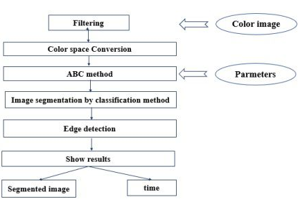
To segment an image into k regions, we applied ABC algorithm using Otsu’s method on different color spaces. This segmentation methodology consists of five steps, as shown in Figure 2: color space conversation, generation of artificial agents in the image ABC method to select optimum thresholds, image segmentation by classification method, and edge detection. These steps are explained at the following subsections.
4.2 Pre-processing of images
To get rid of the noise in the image, we used a multidimensional filter with Gaussian standard deviation equal to 5. The filter allows to reinforce the similarity between the pixels of the same region and to accentuate the differences from different regions. Firstly, we have to define the environment and its states in which bee colony is living and tries to find a solution, before applying ABC method to image segmentation. So, color space is converted from RGB to one of this color space each time (Lab, YCbCr, HSL).
-Color histogram analysis Classes will be constructed by analyzing the color histogram H[I] of the image I.
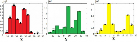
To do this, histograms of each color space components are created (See an example in Figure 3), which describes the distribution of the points-color’s values of each pixel H[I](p) in the image.
Figure 2. Architecture of the proposed methodology
Figure 3. An example of histograms of color components on the three histogram image
4.3 Optimum threshold selection
An artificial bee is coded in three integers from 0 to 255. Hence, the number of optimal thresholds is equal to bee’s number. In order to divide a color set into k homogeneous color clusters, we will take advantages of the two algorithms ABC and multi-level Otsu to propose a hybrid variant. Therefore, ABC method for color clustering is designed as follows:
|
Multi-level Otsu Algorithm |
|
(1). Employed bee phase For each solution: • Randomly select a neighbor $x$different from the current solution. • Create a new solution V according to the equation 1. • Compare the fitness function of the two solutions (current and neighboring). • Keep the best. • If$fit(x)>\,fit(v)$, increment the abandon value of this source$'trai{{l}_{i}}'$. (2). Onlooker bee phase For each solution: • Recalculate the fitness function fit(xi). • Calculate its probability $prob\,(xi)=\frac{\sum{fit(xi)}}{fit(xi)}$ • Apply the roulette selection method. • Randomly select a neighbor Xi different from the current solution. • Create the new solution V according to the equation 1. • Compare the fitness function of the two solutions (current and neighboring).• Keep the best. • If$fit(x)>\,fit(v)$, increment the abandon value of this resource$'trai{{l}_{i}}'$ (3). Scout bee phase For each solution: • If $trai{{l}_{i}}\,<\,~limit$, create a new solution Xi |
-Fitness function: The fitness function is calculated by the Otsu multilevel formula, to determinate the set of thresholds Ti, where $i \in[1, m-1]$ and m is the number of classes. Figure 4 shows an example of multi-le.
vel thresholding segmentation with three thresholds values. Otsu’s method is one of the global non-parametric methods of thresholding, it can find the optimal thresholds value in image without taking in consideration the histogram form [23, 24]. It is based on optimizing the objective function: in this paper we will interest on maximizing the inter-class variance which formulated by the Eq. (5):
$fit\,(xi)=\sum\limits_{k=1}^{K}{{{P}_{k}}}{{({{m}_{k}}-m)}^{2}}$ (5)
where, Pk and mk represent, respectively, the pixels proportion in the classes [Tk1…Tk] and the average intensity of the class itself, and m represents the average intensity of the plane of the image. The pixels proportion Pk of each class is calculated by Eq. (6):
${{P}_{k}}=\,\,\left\{ \begin{align} & \sum\nolimits_{i=1}^{{{t}_{j}}}{\,\,\,\,\,\,\,\,\,\,\,\,\,\,\,\,\,{{P}_{i}}}\,\,\,\,\,\,\,\,\,\,\,\,\,\,\,\,\,\,\,\text{if}\,\,k=1 \\ & \sum\nolimits_{i={{t}_{k-1}}+1}^{{{t}_{j}}}{\,\,\,{{P}_{i}}\,\,\,\,\,\,\,\,\,\,\,\,\,\,\,\,\,\,\,\,\text{if}\,\,1\,<\,k\,<n} \\ & \sum\nolimits_{i={{t}_{k-1}}+1}^{{{t}_{L}}}{\,\,\,{{P}_{i}}\,\,\,\,\,\,\,\,\,\,\,\,\,\,\,\,\,\,\,\,\text{if}\,\,k\,=\,\,n} \\ \end{align} \right.\,$ (6)
The average of each class mk is calculated by Eq. (7):
${{m}_{k}}=\,\,\left\{ \begin{align} & \sum\nolimits_{i=1}^{{{t}_{j}}}{\,\,\,\,\frac{i\times {{P}_{i}}}{{{P}_{k}}}}\,\,\,\,\,\,\,\,\,\,\,\,\,\,\,\,\,\,\,\,\,\,\,\,\,\,\,\,\,\,\,\,\,\text{if}\,\,k=1 \\ & \sum\nolimits_{i={{t}_{k-1}}+1}^{{{t}_{j}}}{\,\,\,\,\frac{i\times {{P}_{i}}}{{{P}_{k}}}\,\,\,\,\,\,\,\,\,\,\,\,\,\,\,\,\,\,\,\,\text{if}\,\,1\,<\,k\,<n} \\ & \sum\nolimits_{i={{t}_{k-1}}+1}^{{{t}_{L}}}{\,\,\,\,\frac{i\times {{P}_{i}}}{{{P}_{k}}}\,\,\,\,\,\,\,\,\,\,\,\,\,\,\,\,\,\,\,\,\text{if}\,\,k\,=\,\,n} \\ \end{align} \right.\,$ (7)
where, L = [0, L-1] represents the intensity levels of the image levels.
4.4 Image segmentation by classification method
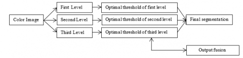
After identifying the optimal thresholds values for each level of the color space. The pixel’s classification will be done according to it. Then, we gather the levels obtained together, in order to get the final image. The Figure 5 explains the segmentation process that we used.
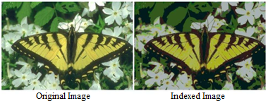
Figure 6 shows original image (on the left) that will be divided into k homogeneous regions (on the right).
Figure 5. Segmentation process in a color space
Figure 6. Segmentation results after pixels classification
In this section, we will make an experimental evaluation of the proposed algorithm. Then, we showed the different obtained results. Finally, we show the quality of our approach by comparing it with Canny’s and ACO algorithm.
5.1 Validation measures
5.1.1 Databases
All experiments have been done on:
-Software: Matlab R2016b.
-System: Windows 10 Professional.
-CPU: Intel Core (TM) i5-6200U CPU@ 2.30GHz, 2.10 GHz
-RAM: 6 Go.
In this section, we present the databases used to train and evaluate the proposed approach. We have done experiments on three different image data-sets. The first one is "Berkeley (BSDS500)" data-set that contains an amount of natural color images, the second one is 3D medical data-set "Drive" contains a digital Retinal Images for Vessel Extraction, and the last one is Oxford-17 flowers which have a 17 category flower data-set, each class has 80 images.
5.1.2 Metric measures for validation step
After segmenting the image, it is necessary to evaluate its quality. For this, we used some evaluation metrics to maximize (PSNR, PR and KI).
-PSNR: (Peak Signal to Noise Ratio): Eq. (8) measures the squared error between the original and the reconstructed image.
$PSNR\,=\,10{{\log }_{10}}\,\frac{{{d}^{2}}}{\tfrac{1}{mn}\sum\nolimits_{i=0}^{m-1}{\sum\nolimits_{j=0}^{n-1}{{{({{I}_{0}}(i,j)-{{I}_{r}}(i,j))}^{2}}}}}$ (8)
where, d is the maximum value of a pixel (d = 255 in this case), I0 and Ir are two images, its height and weight denoted m × n m × n.
-PR: (Performance Ratio): Eq. (9) measures the ratio between the true and the false edge.
$PR\,=\,\frac{TP}{FP+FN}\times 100$ (9)
-KI: (Kappa Index): Eq. (10) measures the similarity between two regions.
$KI\,=\,\frac{2TP}{2TP+FP+FN}\times 100$ (10)
Confusion matrix was built to evaluate treated image that will be compared with Ground Truth (GT) image. The various degree of validation measures are mentioned below.
-TP: the number of correctly classified positives.
-FP: the number of negatives detected by error.
-FN: the number of positives detected by error.
-TN: the number of correctly classified negatives.
5.2 Experimental results and discussion
From a visual point of view of Figure 8, the edge detection results of these images on RGB color space are excellent: It’s accurate to original images, and offer a good quality of discrimination. Also, all the items are directly identifiable. The edge detection results of these images on Lab color space are acceptable but not so precise, as shown in Figure 9: Some pixels which supposed to belong to the image’s objects are arranged in the same class with pixels in the background. All experiments have been done with these parameter set: number of bees = 5, number of iterations = 50, limit=100.
The obtained results of these images on YCbCr color space are quite good, as shown in Figure 10, and give the expected results: We notice that the indexed regions are almost preserved and similar to the original images. Edge detection on HSL color space gives the worst results, as shown in Figure 11: most of the objects of the images are absent or indistinguishable from the background, the quality is blurred. As we can see in Figures 8, 9, 10 and 11, edge detection results are good: edges are well captured and preserved, even though the indexed image didn’t clarify all the details.
Also, the outlines are closed compared to another algorithm like ACO, as shown in Figure 7. All the measurements of the performances of our approach and other algorithm illustrated in the Tables 1, 2 and 3.
You can notice that the PSNR values are very close to each other, generally between 19.93 db and 20.4585 db. For PR metric, results are so various. In the other hand, KI metric has a fast increase, from 7.8151e-05 for ACO algorithm to 0.22761 for the RGB color space. The Running Time (RT) has also improved. From these experiences, we can say that segmentation on grayscale Image (GI) ACO gives the worst results.
Table 1. Evaluation of metric values for first image segmented in different color space
|
Image 1 |
|||||
|
|
|
PSNR |
PR |
KI |
RT |
|
ABC |
RGB |
20.0842 |
40.4007 |
0.12291 |
0.081060 |
|
Lab |
20.1887 |
34.8503 |
0.13445 |
2.881643 |
|
|
YCbCr |
20.0948 |
42.8596 |
0.12771 |
1.11867 |
|
|
HSL |
20.0494 |
19.0498 |
0.07138 |
1.836927 |
|
|
ACO |
GI |
19.9307 |
43.2188 |
9.132e-05 |
231.8590 |
|
Canny |
GI |
17.214 |
12.5393 |
0.0491 |
0.070703 |
|
Image 2 |
|||||
|
|
|
PSNR |
PR |
KI |
RT |
|
ABC |
RGB |
20.049 |
31.383 |
0.07336 |
0.45589 |
|
Lab |
20.153 |
28.9061 |
0.07598 |
1.67696 |
|
|
YCbCr |
20.154 |
30.8656 |
0.04972 |
1.94172 |
|
|
HSL |
20.071 |
33.0369 |
0.06333 |
0.82076 |
|
|
ACO |
GI |
20.019 |
16.9918 |
7.8151e-05 |
155.584 |
|
Canny |
GI |
19.916 |
10.3822 |
0.0491 |
0.10068 |
|
Image 3 |
|||||
|
|
|
PSNR |
PR |
KI |
RT |
|
ABC |
RGB |
20.255 |
34.3363 |
0.14739 |
0.081060 |
|
Lab |
20.325 |
31.6224 |
0.13454 |
0.755214 |
|
|
YCbCr |
20.458 |
36.0279 |
0.13485 |
0.943834 |
|
|
HSL |
20.425 |
33.1885 |
0.12087 |
1.000217 |
|
|
ACO |
GI |
20.118 |
7.7207 |
14.415e-05 |
21.65919 |
|
Canny |
GI |
20.252 |
55.5614 |
0.023326 |
0.141228 |
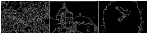
Figure 7. First line: Original images, second line: Edge detection by ACO method in greylevel color space
Figure 8. Edge detection results by ABC method in RGB color space
Figure 9. Edge detection results by ABC method in L∗a∗b∗ - CIE color space
Figure 10. Edge detection results by ABC method in YCbCr color space
Figure 11. Edge detection results by ABC method in HSL color space
In this work, we studied a theme well addressed in the resolution of image segmentation’s problem by meta-heuristics algorithm. In the first part, we give a general idea about the image processing domain, especially edge detection and thresholding. Also, we described ABC algorithm and how to apply in color image segmentation. Then, our algorithm has been tested on several images of the Berkeley and others databases. Finally, we used the "Ground Truth", a synthetic non-noisy image to compare between it and carried out image. The experimental results showed that our algorithm is highly efficient in Running Time and edge detection quality. By using different color spaces in the search area, our algorithm can be successfully applied to multi-level image thresholding then boundaries detection. Through visual experimental and numerical quantitative comparisons According evaluated results we have proved that the significant color space considered in this study are RGB, YCbCr and Lab as it’s shown in Figure 7 to Figure 11, also we have proven that our approach shows obvious superiority over ACO and Canny method.
[1] Senthilkumaran, N., Vaithegi, S. (2016). Image segmentation by using thresholding techniques for medical images. Computer Science & Engineering: An International Journal, 6(1): 1-13. https://doi.org/10.5121/cseij.2016.6101
[2] Akay, B. (2013). A study on particle swarm optimization and artificial bee colony algorithms for multilevel thresholding. Applied Soft Computing, 13(6): 3066-3091. https://doi.org/10.1016/j.asoc.2012.03.072
[3] Sarkar, S., Das, S., Chaudhuri, S.S. (2015). A multilevel color image thresholding scheme based on minimum cross entropy and differential evolution. Pattern Recognition Letters, 54: 27-35. http://dx.doi.org/10.1016/j.patrec.2014.11.009
[4] Sharma, T.K., Pant, M. (2017). Shuffled artificial bee colony algorithm. Soft Computing, 21: 6085-6104. http://dx.doi.org/10.1007/s00500-016-2166-2
[5] Ye, Z., Hu, Z., Wang, H., Chen, H. (2011). Automatic threshold selection based on artificial bee colony algorithm. 3rd International Workshop on Intelligent Systems and Applications, Wuhan, China, pp. 1-4. http://dx.doi.org/10.1109/ISA.2011.5873357
[6] Zhang, Y., Wu, L. (2011). Optimal multi-level thresholding based on maximum tsallis entropy via an artificial bee colony approach. Entropy, 13: 841-859. http://dx.doi.org/10.3390/e13040841
[7] Ma, M., Liang, J., Guo, M., Fan, Y., Yin, Y. (2011). SAR image segmentation based on artificial bee colony algorithm. Applied Soft Computing, 11(8): 5205-5214. http://dx.doi.org/10.1016/j.asoc.2011.05.039
[8] Lu, X.M., Wu, Q., Zhou, Y., Yao, M., Song, C.C., Ma, C. (2019). A dynamic swarm firefly algorithm based on chaos theory and max-min distance algorithm. Traitement du Signal, 36(3): 227-231. https://doi.org/10.18280/ts.360304
[9] Chidambaram, C., Lopes, H.S. (2009). A new approach for template matching in digital images using an artificial bee colony algorithm. World Congress on Nature Biologically Inspired Computing, Coimbatore, India, pp. 146-151. http://dx.doi.org/10.1109/NABIC.2009.5393631
[10] Karima, B., Hamid, S. (2019). Improvement on image edge detection using a novel variant of the ant colony system. Journal of Circuits, Systems and Computers, 28(5): 1950080. https://doi.org/10.1142/S0218126619500804
[11] Yigitbasi, E.D., Baykan, N.A. (2013). Edge detection using artificial bee colony algorithm (ABC). International Journal of Information and Electronics Engineering, 3(6): 634-638. http://dx.doi.org/10.7763/IJIEE.2013.V3.394
[12] Singh, R.A., Vashishath, M., Kumar, S. (2019). Ant colony optimization technique for edge detection using fuzzy triangular membership function. International Journal of System Assurance Engineering and Management, 10: 91-96. https://doi.org/10.1007/s13198-019-00768-y
[13] Gonzalez, C.I., Castro, J.R., Melin, P., Castillo, O. (2015). Cuckoo search algorithm for the optimization of type-2 fuzzy image edge detection systems. IEEE Congress on Evolutionary Computation 2015, Sendai, Japan, pp. 449-455. http://dx.doi.org/10.1109/CEC.2015.7256924
[14] Perez, J., Valdez, F., Castillo, O. (2017). Interval type-2 fuzzy logic for dynamic parameter adaptation in the bat algorithm. Soft Computing, 21: 667-685. https://doi.org/10.1007/s00500-016-2469-3
[15] Mao, R. (2017). A swarm intelligence based medical image edge detection method with adaptive gradient. Journal of Medical Imaging and Health Informatics, 7(4): 1087-1092. http://dx.doi.org/10.1166/jmihi.2017.2141
[16] Chen, T., Sun, X.K., Han, H., You, X.M. (2015). Image edge detection based on ACO-PSO algorithm. Image, 6(7): 47-54. http://dx.doi.org/10.14569/IJACSA.2015.060708
[17] Rajasekhar, A., Lynn, N., Das, S., Suganthan, P.N. (2017). Computing with the collective intelligence of honey bees- A survey. Swarm and Evolutionary Computation, 32: 25-48. http://dx.doi.org/10.1016/j.swevo.2016.06.001
[18] Alzaqebah, M., Abdullah, S., Jawarneh, S. (2016). Modified artificial bee colony for the vehicle routing problems with time windows. Springerplus, 5(1): 1298. http://dx.doi.org/10.1186/s40064-016-2940-8
[19] Lien, L.C., Cheng, M.Y. (2014). Particle bee algorithm for tower crane layout with material quantity supply and demand optimization. Automation in Construction, 45: 25-32. http://dx.doi.org/10.1016/j.autcon.2014.05.002
[20] Schiezaro, M., Pedrini, H. (2013). Data feature selection based on artificial bee colony algorithm. Euracip Journal on Image and Video Processing, 47: 1-8. http://dx.doi.org/10.1186/1687-5281-2013-47
[21] Davidović, T. (2016). Bee colony optimization part i: The algorithm overview. Yugoslav Journal of Operations Research, 25(1): 33-56. http://dx.doi.org/10.2298/YJOR131011017D
[22] Li, L., Sun, L., Guo, J., Han, C., Zhou, J., Li, S. (2017). A quick artificial bee colony algorithm for image thresholding. Information, 8(1): 1-19. http://dx.doi.org/10.3390/info8010016
[23] Berrak, O., Belmeguenai, A., Ouchtati, S. (2019). Secure transfer of color images using horizontal and vertical scan. Traitement du Signal, 36(1): 45-51. https://doi.org/10.18280/ts.360106
[24] Staal, J., Abramoff, M., Niemeijer, M., Viergever, M., van Ginneken, B. (2004). Ridge based vessel segmentation in color images of the retina. IEEE Transactions on Medical Imaging, 23: 501-509. http://dx.doi.org/10.1109/TMI.2004.825627