Moosa Katouli* | Akram Esvand Rahmani
© 2020 IIETA. This article is published by IIETA and is licensed under the CC BY 4.0 license (http://creativecommons.org/licenses/by/4.0/).
OPEN ACCESS
Brain diseases are common causes of death and burns such as cancerous tumors. Nowadays, the use of automated computer techniques is quite common for faster extraction and better identification of tumor locations. The present study examines the diagnosis of brain tumors in MRI imaging through a super pixel-based clustering technique. In the proposed method, additional regions of MRI images were removed by pre-processing operations to eliminate noise and skull removal to increase the speed of tumor detection. Then, the super pixels were calculated by dividing the image into even blocks. Spectral clustering was performed on the ROI containing the tumor tissue information. Finally, adjacent blocks were identified by Filter Gabor to identify brain tumors in MRI images. Based on the results, the proposed method has shown better performance in terms of accuracy, sensitivity, and specificity in comparison to other methods. The function of brain tumor diagnosis can be useful in helping physicians identify more rapidly.
brain tumor, super pixel, spectral clustering, filter Gabor
The human body is made up of several types of cells, including brain cells which are placed in a highly specialized organ of the human body. A brain tumor is a harmful disease for humans; it is a mass within the skull that consists of abnormal tissue growth in or around the brain. A brain tumor is usually caused by the growth of brain cells, blood vessels, and nerves [1].
A brain tumor can be either benign or malignant, the malignant type being more dangerous than the benign one due to its high rate of transmission to other brain tissues [2]. Diagnosing a brain tumor is a complex task due to the shape, size, and location of the tumor in the brain. Diagnosis at the onset is much more difficult because the tumor cannot be identified accurately. But once the tumor is identified and appropriate treatment is started, the benign and sometimes malignant tumor can be treatable. Tumors are treated with chemotherapy, radiation, and surgery, depending on the type of tumor.
In recent years, the tumor range in the brain image has been determined manually in clinical applications; but manual procedures are virtually impossible when the volume of information and images is high. Therefore, an automated system is needed to detect the tumor range in brain images. On the other hand, MRI is an imaging technique that allows for clear imaging in different parts of the body surrounded by bone tissue. For this reason, MRI scans are the best imaging technique to detect benign and malignant tumors in the brain.
Tumor diagnosis is one of the most important applications of image processing in the medical field, and this application is considered when photographs taken by different require medical devices that all details of the image be evident and clear [3]. There is a need for a method that can accurately identify and diagnose tumors because brain tumors are sensitive, one of the challenges is that the location of the tumors is different. Different tumors shape and size have different patterns, and it is complicated to distinguish between healthy tumors and brain tissues [4].
In methods of medical image segmentation such as deep learning [5], due to the prolongation of image processing time when working with large data sets, pixel-based spectral clustering is more appropriate. Also, in other spectral clustering methods, since there is no hypothesis concerning cluster shapes, when the data set is enlarged, a special vector generalization is needed which can withstand the heavy computational load.
In 2015, Ayşe et al. [4] Presented a spectral clustering-based method for brain tumor detection. In this method, the ROI (Region of Interest) is divided by spectral clustering rather than the whole image, which contains information from the tumor tissue. Data reduction is made using super pixels, which are produced using the Central Tendency Value (CTV) of image blocks. These super pixels are considered as nodes for spectral clustering to detect ROI. As a result, super pixels, tumor super pixels, and non-tumor super pixels are obtained. The main block of tumor super pixels in the image is designated as the tumor block.
The proposed method can increase speed and accuracy, as well as identify the brain tumor area through the clustering algorithm [4]. Finally, morphological operations are applied to make the ROI more accurately.
This paper is organized as follows: Section 2 described an overview of known methods of dimensionality reduction. In Section 3, the effect of the grasshopper optimization algorithm on dimensionality reduction investigated in lung cancer diagnosis systems. Section 4 the evaluation of the methods investigated along with the results table, comparisons, and their analysis. Finally, the conclusions presented in Section 5.
This section examined several methods of tumor diagnosis in MRI images and then points out the weaknesses of these methods for tumor identification.
A method was applied for classifying brain tumor images through deep learning [5]. This method was tested on three different datasets. In this method, a new architecture has been created for crop, uncrop and partitioning using 18 layers so that the classification can effectively grade the brain tumor.
The highest accuracy of the proposed method was 99% on the images that were uncropped.
A method has been presented to diagnose and segment brain tumors [6]. In this method, the combined clustering method of FCM, k-means and active contour has been used for segmentation. In this method, the execution time has been reduced due to the combinational effect.
SVM classification is used with morphological transformations and GLCM tissue properties to classify brain images [7]. In this study, after the pre-processing which is done by morphological operations, features such as entropy, contrast, energy, homogeneity, etc. are extracted. These features are then given to the SVM classifier to be converted into normal and non-normal categories.
The surveillance method requires massive datasets with valid ground truth [8]. Managing tagged datasets is a challenging and time-consuming task if done manually. On the other hand, the unsupervised method does not depend on the training dataset and can be applied to different imaging data sets [9]. Unsupervised clustering methods can be used to reduce complexity and speed up execution without losing precision for evaluation as spectral clustering, which achieved a global optimization solution, among other clustering techniques. Spectral Clustering Performs data grouping (clusters) using Laplace data. The properties of the Laplace matrix provide important information about the relevant components of the given data. A set of eigenvalues of the Laplace matrix is called the "spectrum" of the graph, and the name is "spectral cluster." The primary limitation of the spectral clustering is the dense dependence matrix structure.
In 2016, Sauwen et al. proposed GMM (Gaussian Mixture Model) clustering to produce competitive results with advanced unsupervised algorithms for brain tissue segmentation [10].
Spectral clustering of super pixels is used to segment the brain tumor-based ROI into [11]. The method uses spectral clustering and successful super pixels in the segmentation process.
The proposed method is inspired by the method proposed by Angulakshmi et al. [11] In the proposed method, additional areas are removed from MRI images using pre-processing noise ablation and skull removal to increase the speed of tumor detection, which is not addressed in the procedure.
In addition, splitting the image into the same blocks can be computed by super pixels. Spectral clustering is performed on the ROI containing the tumor tissue information. Finally, the adjoining blocks are identified by a local binary pattern (LBP) [11]; instead, the proposed method uses a Gabor filter to make the brain tumor diagnosis in MRI images more accurate. The details of the proposed method are described in the next section.
The advantage of spectral clustering over other methods is its use of a super-pixel-like similarity matrix, which, in addition to reducing execution time, leads to an optimal solution between anatomical connections between pixels.
In the pre-processing section, the NLM filter is first filtered to eliminate MRI image noise. In addition, skull removal is performed to increase the speed of the work using morphological operations. Segmentation is then performed using spectral clustering on the ROI (area of interest) obtained from the calculation of super pixels on the blocks. In the last step, LBP was used by Angulakshmi and Priya [11], whereas the Gabor filter is used in the proposed method to extract features and identify adjacent blocks for increasing classification recognition and accuracy.
3.1 Pre-processing
The use of Gaussian filters is widespread in FMR (Functional magnetic resonance) images, but it blurs the edges of the image by averaging. Impermeable filters are used to solve this problem. The method is very useful for maintaining the edges [12]. However, such a filter usually removes minor features and renders the image abnormal due to the enhanced edge effect.
This section aimed to examine the new Non Local Means (NLM) filter, which performs better than other classic methods such as Total Variation (TV) and Wavelet.
In this step, a discrete windowed cosine converter with thresholding was used as a thinning conversion. Then the non-local median parameter was used, which is a filter highly dependent on parameter adjustment.
The NLM filter is a filter based on the mean of the same pixels based on their distance intensity. The NLM filter calculated the average weight of all pixels of the image based on Formula (1):
NLM(Y(p)) = ∑ W(p,q)Y(q) ∀q ∈Y
0 ≤ w (p, q) ≤1 ∑ w (p, q) = 1 ∀q ∈Y (1)
In relation (1), the target of p is filtered, and q represents each pixel of the image. W (p, q) based on the similarity between the Np and Nq neighbors of the pixel’s p and q. The similarity of w (p, q) is calculated by the formula (2):
$W(p, q)=1 / Z(p) e-d(p, q) \cdot / h^{2}$ (2)
Z (p) ∀q, is constant.
$d(p, q)-D p\|Y(N p)-(N q)\| 2 R \operatorname{sim}$ (3)
When q=p, it indicated that the self-similarity property is very high, and for this case, the condition w (p, q) of formula four is calculated:
$w(p, p)=\max (p, q) \forall q \neq p$ (4)
NLM filter can increase SNR without affecting the original image structure in MRI images. An ideal filter works to preserve image features. Since no objective criterion fully meets this requirement, the difference between the original image and the filtered image is used to evaluate the performance of the filter [13]. Therefore, the NLM filter can be the best way to substantially reduce image noise by averaging similar pixels [12].
Due to their striking similarity to the brain structure, skulls, skin, and other non-brain tissues can, in some methods, lead to incorrect partitioning, and/or increase the minimum processing time. In this system, all deletions were accomplished using open and closed morphological operations resulting from relationships (5) and (6).
$A \cdot B=(A \ominus B) \oplus B$ (5)
Operations resulting from erosion and then dilation of complex A were calculated by structural elements B are called open operations, which was used in the proposed method to remove small objects from MRI images.
$A \cdot B=(A \oplus B) \ominus B$ (6)
Operations resulting from dilution and then erosion of complex A were calculated by the structural elements B, which called open operations, which was used in the proposed method for filling the pits.
3.2 Identify the region of interest
When the image size was reduced relative to the original image, and the abnormal region of the MRI image was displayed, that region was the region of interest (ROI). Image processing is usually confined to a small area, which is our area of interest (ROI).
In the ROI identification process, the non-tumor segment in the segmentation process was eliminated. In this method, the ROI was obtained using spectral clustering rather than the whole image which contains information from the tumor tissue. The process of identifying the area of interest or ROI involved four basic steps:
3.2.1 Calculate super pixels
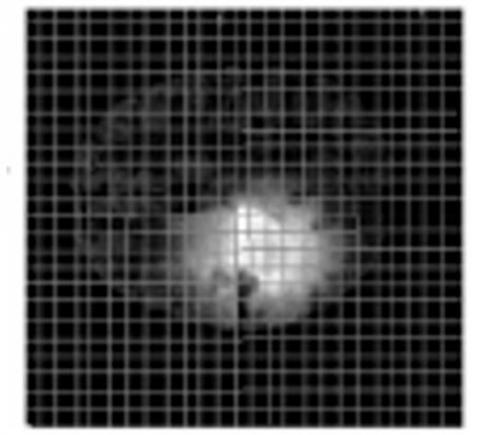
In this section, the image was divided into blocks of the same size, which have been shown in Figure 1. Super pixels are produced using the Central Tendency Value (CTV) of image blocks. The central Tendency Value (CTV) usually tends to the key value of the data. In the proposed method, the central value was calculated using mean, median, and mode, and the corresponding block was used as the super pixel value.
Figure 1. A blocked MRI image [11]
If B1, B2, B3, …, Bm are blocks of the image, m represents the number of blocks. The intensity values of the pixels P1, P2, Pn were considered in terms n denotes the number of pixels per block. The central value was represented by Mi as estimated by the average of all the pixels in each block.
$M_{i}=\frac{1}{n} \sum_{j=1}^{n} P_{j}^{i}$ (7)
In the above relation, i=1, 2, …, m represents the number of blocks in the image. $P_{j}^{i}$ is the value of the jth pixel of the ith block in the image?
Now, the central value is calculated using the Medi median value as follows:
$\mathrm{Med}_{\mathrm{i}}=\left\{\begin{array}{ll}\frac{1}{2}\left(\mathrm{P}_{\mathrm{i}}^{\frac{\mathrm{n}}{2}}\right)\left(\mathrm{P}_{\mathrm{i}}^{\frac{\mathrm{n}}{2}+1}\right), & \text { if } \mathrm{n} \% 2=0 \\ \left(\mathrm{P}_{\mathrm{i}}^{\frac{\mathrm{n}+1}{2}}\right), & \text { if } \mathrm{n} \% 2 \neq 0\end{array}\right\}$ (8)
In the above relation, n=1, 2, ..., n is the i-min block. $P_{i}^{\frac{n}{2}}$, $\frac{n}{2}$ is the pixel value of ith block. $P_{i}^{\frac{n}{2}+1}$, $\frac{n}{2}+1$ is the pixel value of ith block. Also $P_{i}^{\frac{n+1}{2}}$, $\frac{n+1}{2}$ is the pixel value of ith block.
Finally, the median value was calculated using the Modei median as follows:
Modei= Most frequently occurring pixel value Pi in ith the block Bi of the image I (9)
In the above relation, i=1, 2, …, m represents the number of blocks in each image.
Finally, the super pixels are segmented using spectral clustering.
3.2.2 Separation of super pixels
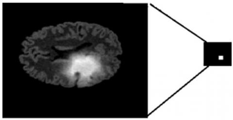
Spectral segmentation was performed on the super pixel values of the image blocks. Segmentation of the super pixels was performed to obtain tumor super pixels and non-tumor super pixels. An example of the segmentation results of the tumor- super pixels has been given in Figure 2.
Figure 2. The results of segmentation of the tumor- superpixels [11]
The white area in the image represents the brain tumor, and the blue indicates the non-tumor area.
3.2.3 Identify tumor block
The block of the image was identified in the original image where the tumor's super pixel belongs. The tumor blocks can be featured similar to the tumor block to display ROI since the tumor block can be expanded. Therefore, LBP was used to increase the accuracy and detection of a Gabor filter to identify similar features [11].
3.2.4 Identify adjacent blocks
The image orientation features can be extracted at different scales using Gabor's two-dimensional wavelet transform. Physiology researches have indicated that visual information processing in the visual system is accomplished by a set of parallel mechanisms called channels. Each channel is tuned for a low-bandwidth band with a specific direction. Mathematically, each of these channels is modeled with a pair of Gabor pass-through filters. Invariance over image brightness, rotation, scaling, and image transfer is the most important advantage of Gabor filters. In addition, these filters can withstand photometric distortions such as brightness and noise changes in the image. In the spatial coordinate domain of a two-dimensional Gabor filter, it is a Gaussian kernel function modulated by a complex sinusoidal flat wave, which is in Formula (10):
$G(\mathrm{x}, \mathrm{y})=\frac{\mathrm{f}^{2}}{\pi \gamma \mu} \exp \left(-\frac{\mathrm{x}^{\prime2}+\mathrm{y}^{\prime 2}}{2 \delta^{2}}\right) \exp \left(\mathrm{j} 2 \pi \mathrm{fx}^{\prime}+\varphi\right)$
$\mathrm{x}^{\prime}=x \cos \theta+y \sin \theta$
$\mathrm{y}^{\prime}=-x \sin \theta+y \cos \theta$ (10)
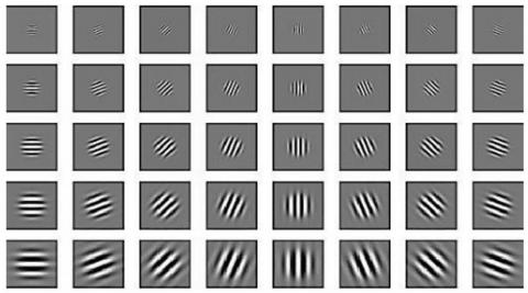
where, f is the frequency of the sinusoidal factor. θ also shows the comparison of normal stripes of the Gabor function with respect to the parallel stripes of the Gabor function. "φ" is the phase offset, and δ is equal to the Gaussian standard deviation. γ is the ratio of the spatial visibility that determines the elliptic support of the Gabor function. As shown in Figure 3, the algorithm can use forty Gabor filters in five scales and eight directions [14].
Figure 3. Gabor filter in 5 Scale and 8 directions
Since the adjacent pixels in the image are correlated to each other, the information of the plug-in can be eliminated through the less-than-usual sampling process of images resulting from Gabor filters.
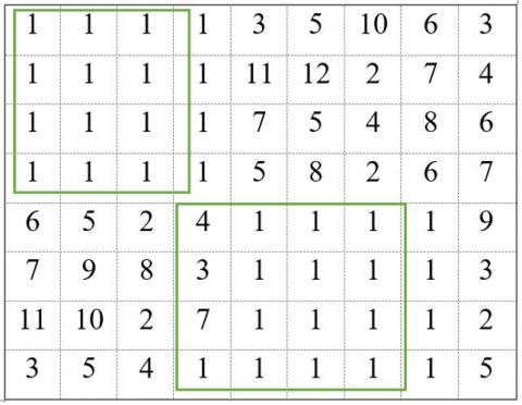
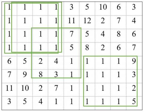
In the proposed method, the wavelet transform was converted to L after reading the input image with the size M×N; then the blocks continued as b×b pixels from the upper left corner and above the lower right corner of the image for each position. The block was mapped to the fifth row of the Gabor filter, and the pixel values were extracted in a row from the two-dimensional A matrix consisting of 32 columns and (M-B+1)×(N-B+1) rows. Each row corresponded to a block position to better understand the implementation steps of the proposed method. This algorithm was illustrated with a straightforward and small image, as in Figure 4.
Figure 4. 8×9 image
A 4×4 window based on an image by image scheme was moved applying the Gabor filter on each block because Figure 4 is so small (Block 8×8 was used in the original code). The overlapping blocks were inserted as a row vector into the attribute matrix as shown in Figure 5.
Figure 5. Overlap blocking row by row
The obtained character matrix from the previous alphabetical sorting procedure was applied to ensure the minimum number of comparisons to find the most similar blocks to each other, thereby aligning the rows most similar to each other and running the algorithm in time. The result can be reduced significantly, and the result of the alphabetical sorting performed on the image property matrix is in Table 1 and Table 2.
As can be seen from Table 1 and Table 2, blocks 2 and 26 are examples of similar blocks. Regions with the same blocks are labeled as tumor regions, and non-similar blocks are labeled as non-tumor regions.
Fourier transforms, and phase correlation relationships were used to find the most similar blocks. In the previous step, the feature vectors were arranged alphabetically. The similarity of the blocks to each other was used to match the pattern [15].
$s=s_{1}, s_{2}=x_{i}-x_{j}, y_{i}-y_{j}$ (11)
In the above relation, s1 and s2 are the desired blocks. The vector coordinates xi and xj are the corresponding properties of yi and yj. An image threshold was defined for the image to be forged, which is mostly empirical when selecting this coefficient.
Table 1. Matrix of feature vectors before sorting
|
Matrix of Feature vectors before sorting |
Block index |
|||||||||||||||
|
1 |
1 |
1 |
1 |
1 |
1 |
1 |
1 |
1 |
1 |
1 |
1 |
1 |
1 |
1 |
1 |
1 |
|
3 |
5 |
2 |
6 |
1 |
1 |
1 |
1 |
1 |
1 |
1 |
1 |
1 |
1 |
1 |
1 |
2 |
|
4 |
8 |
6 |
5 |
4 |
3 |
2 |
5 |
4 |
1 |
1 |
1 |
1 |
1 |
1 |
1 |
3 |
|
5 |
6 |
1 |
2 |
10 |
12 |
2 |
8 |
4 |
9 |
3 |
4 |
1 |
1 |
1 |
1 |
4 |
|
12 |
3 |
4 |
6 |
11 |
6 |
7 |
5 |
3 |
7 |
5 |
2 |
6 |
1 |
1 |
1 |
5 |
|
1 |
6 |
5 |
9 |
3 |
4 |
5 |
6 |
12 |
10 |
8 |
1 |
1 |
4 |
3 |
1 |
6 |
|
3 |
2 |
2 |
5 |
6 |
9 |
8 |
7 |
11 |
12 |
8 |
9 |
4 |
3 |
5 |
6 |
7 |
|
9 |
1 |
2 |
3 |
4 |
9 |
11 |
10 |
8 |
7 |
3 |
1 |
7 |
4 |
2 |
5 |
8 |
|
7 |
2 |
3 |
4 |
8 |
7 |
5 |
6 |
4 |
2 |
1 |
7 |
2 |
5 |
3 |
10 |
9 |
|
6 |
2 |
4 |
8 |
3 |
4 |
2 |
9 |
6 |
7 |
8 |
5 |
4 |
2 |
1 |
6 |
10 |
|
7 |
3 |
12 |
11 |
9 |
7 |
5 |
8 |
1 |
7 |
2 |
5 |
1 |
9 |
6 |
4 |
11 |
|
1 |
8 |
3 |
6 |
4 |
1 |
9 |
9 |
4 |
5 |
8 |
1 |
6 |
4 |
10 |
5 |
12 |
|
5 |
1 |
3 |
7 |
9 |
12 |
9 |
7 |
4 |
9 |
2 |
7 |
3 |
4 |
6 |
1 |
13 |
|
7 |
2 |
5 |
11 |
3 |
12 |
10 |
9 |
6 |
2 |
9 |
7 |
3 |
1 |
2 |
5 |
14 |
|
5 |
122 |
2 |
11 |
1 |
3 |
9 |
7 |
6 |
3 |
4 |
2 |
8 |
7 |
1 |
1 |
15 |
|
8 |
2 |
2 |
3 |
4 |
1 |
9 |
8 |
7 |
6 |
5 |
11 |
9 |
8 |
6 |
8 |
16 |
|
3 |
4 |
5 |
1 |
2 |
8 |
7 |
6 |
2 |
3 |
4 |
1 |
9 |
7 |
3 |
6 |
17 |
|
1 |
2 |
9 |
8 |
7 |
6 |
5 |
5 |
4 |
9 |
8 |
3 |
7 |
5 |
2 |
5 |
18 |
|
10 |
11 |
4 |
12 |
9 |
5 |
2 |
4 |
3 |
2 |
9 |
7 |
8 |
6 |
2 |
4 |
19 |
|
12 |
10 |
4 |
5 |
7 |
9 |
3 |
8 |
2 |
7 |
2 |
3 |
5 |
9 |
6 |
4 |
20 |
|
9 |
3 |
7 |
5 |
2 |
5 |
8 |
2 |
9 |
4 |
9 |
2 |
8 |
7 |
5 |
3 |
21 |
|
7 |
2 |
5 |
6 |
7 |
12 |
11 |
9 |
8 |
6 |
7 |
5 |
2 |
3 |
2 |
7 |
22 |
|
8 |
4 |
2 |
4 |
7 |
6 |
3 |
9 |
8 |
2 |
7 |
4 |
8 |
7 |
3 |
4 |
23 |
|
2 |
7 |
4 |
9 |
6 |
7 |
10 |
12 |
11 |
8 |
3 |
5 |
9 |
7 |
4 |
2 |
24 |
|
6 |
10 |
9 |
8 |
2 |
3 |
7 |
4 |
3 |
10 |
5 |
2 |
9 |
2 |
7 |
6 |
25 |
|
2 |
7 |
5 |
8 |
3 |
9 |
7 |
4 |
5 |
9 |
9 |
6 |
4 |
3 |
2 |
9 |
26 |
|
5 |
6 |
8 |
11 |
10 |
12 |
2 |
3 |
4 |
7 |
9 |
8 |
6 |
5 |
4 |
3 |
27 |
|
4 |
8 |
7 |
10 |
7 |
5 |
3 |
5 |
1 |
2 |
7 |
9 |
7 |
6 |
5 |
2 |
28 |
|
5 |
4 |
3 |
2 |
4 |
9 |
8 |
2 |
6 |
4 |
3 |
6 |
12 |
7 |
10 |
11 |
29 |
|
4 |
3 |
2 |
5 |
6 |
9 |
12 |
7 |
11 |
7 |
10 |
5 |
2 |
3 |
9 |
7 |
30 |
|
Matrix of Feature vectors After sorting |
Block index |
|||||||||||||||
|
1 |
1 |
1 |
1 |
1 |
1 |
1 |
1 |
1 |
1 |
1 |
1 |
1 |
1 |
1 |
1 |
1 |
|
3 |
5 |
2 |
6 |
1 |
1 |
1 |
1 |
1 |
1 |
1 |
1 |
1 |
1 |
1 |
1 |
2 |
|
4 |
8 |
6 |
5 |
4 |
3 |
2 |
5 |
4 |
1 |
1 |
1 |
1 |
1 |
1 |
1 |
3 |
|
5 |
6 |
1 |
2 |
10 |
12 |
2 |
8 |
4 |
9 |
3 |
4 |
1 |
1 |
1 |
1 |
4 |
|
12 |
3 |
4 |
6 |
11 |
6 |
7 |
5 |
3 |
7 |
5 |
2 |
6 |
1 |
1 |
1 |
5 |
|
5 |
122 |
2 |
11 |
1 |
3 |
9 |
7 |
6 |
3 |
4 |
2 |
8 |
7 |
1 |
1 |
15 |
|
3 |
2 |
2 |
5 |
6 |
9 |
8 |
7 |
11 |
12 |
8 |
9 |
4 |
3 |
5 |
6 |
7 |
|
5 |
1 |
3 |
7 |
9 |
12 |
9 |
7 |
4 |
9 |
2 |
7 |
3 |
4 |
6 |
1 |
13 |
|
1 |
6 |
5 |
9 |
3 |
4 |
5 |
6 |
12 |
10 |
8 |
1 |
1 |
4 |
3 |
1 |
6 |
|
9 |
3 |
7 |
5 |
2 |
5 |
8 |
2 |
9 |
4 |
9 |
2 |
8 |
7 |
5 |
3 |
21 |
|
2 |
7 |
5 |
8 |
3 |
9 |
7 |
4 |
5 |
9 |
9 |
6 |
4 |
3 |
2 |
9 |
26 |
|
7 |
3 |
12 |
11 |
9 |
7 |
5 |
8 |
1 |
7 |
2 |
5 |
1 |
9 |
6 |
4 |
11 |
|
4 |
8 |
7 |
10 |
7 |
5 |
3 |
5 |
1 |
2 |
7 |
9 |
7 |
6 |
5 |
2 |
28 |
|
6 |
10 |
9 |
8 |
2 |
3 |
7 |
4 |
3 |
10 |
5 |
2 |
9 |
2 |
7 |
6 |
25 |
|
7 |
2 |
5 |
11 |
3 |
12 |
10 |
9 |
6 |
2 |
9 |
7 |
3 |
1 |
2 |
5 |
14 |
|
8 |
2 |
2 |
3 |
4 |
1 |
9 |
8 |
7 |
6 |
5 |
11 |
9 |
8 |
6 |
8 |
16 |
|
8 |
4 |
2 |
4 |
7 |
6 |
3 |
9 |
8 |
2 |
7 |
4 |
8 |
7 |
3 |
4 |
23 |
|
10 |
11 |
4 |
12 |
9 |
5 |
2 |
4 |
3 |
2 |
9 |
7 |
8 |
6 |
2 |
4 |
19 |
|
9 |
1 |
2 |
3 |
4 |
9 |
11 |
10 |
8 |
7 |
3 |
1 |
7 |
4 |
2 |
5 |
8 |
|
1 |
2 |
9 |
8 |
7 |
6 |
5 |
5 |
4 |
9 |
8 |
3 |
7 |
5 |
2 |
5 |
18 |
|
7 |
2 |
5 |
6 |
7 |
12 |
11 |
9 |
8 |
6 |
7 |
5 |
2 |
3 |
2 |
7 |
22 |
|
7 |
2 |
3 |
4 |
8 |
7 |
5 |
6 |
4 |
2 |
1 |
7 |
2 |
5 |
3 |
10 |
10 |
|
4 |
3 |
2 |
5 |
6 |
9 |
12 |
7 |
11 |
7 |
10 |
5 |
2 |
3 |
9 |
7 |
30 |
|
2 |
7 |
4 |
9 |
6 |
7 |
10 |
12 |
11 |
8 |
3 |
5 |
9 |
7 |
4 |
2 |
24 |
|
7 |
2 |
3 |
4 |
8 |
7 |
5 |
6 |
4 |
2 |
1 |
7 |
2 |
5 |
3 |
10 |
9 |
|
12 |
10 |
4 |
5 |
7 |
9 |
3 |
8 |
2 |
7 |
2 |
3 |
5 |
9 |
6 |
4 |
20 |
|
5 |
6 |
8 |
11 |
10 |
12 |
2 |
3 |
4 |
7 |
9 |
8 |
6 |
5 |
4 |
3 |
27 |
|
1 |
8 |
3 |
6 |
4 |
1 |
9 |
9 |
4 |
5 |
8 |
1 |
6 |
4 |
10 |
5 |
12 |
|
3 |
4 |
5 |
1 |
2 |
8 |
7 |
6 |
2 |
3 |
4 |
1 |
9 |
7 |
3 |
6 |
17 |
|
5 |
4 |
3 |
2 |
4 |
9 |
8 |
2 |
6 |
4 |
3 |
6 |
12 |
7 |
10 |
11 |
29 |
3.3 Region of interest (ROI)
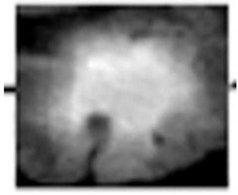
Spectral clustering was applied to the area of interest to increase processing speed and segmentation accuracy directly. All pixel values in the field of interest were considered to construct a similarity matrix for spectral clustering. The matrix of similarity can be prevented when the area of interest is small. Spectral clustering was performed to increase accuracy and quality, and there was no approximation in the construction of the similarity matrix to prevent dense similarity matrix formation. In spectral clustering, at first, a dependency matrix is created, and the problem is transferred into a graph bringing together the interconnected components of the graph forming a cluster by constructing this dependency matrix. In this graph, edges with elements in one cluster are weighted, and, in contrast, edges which lacked elements in a cluster are less weighty. Then the Laplacian graph is created, and the special vectors are selected for it. Finally, a clustering algorithm such as K-means can be obtained through special vectors. Ultimately, this algorithm must be obtained the expected number of clusters from the user, but the optimal number can be selected for the number of clusters using the space between particular vectors. Figure 6 shows the results of the ROI segmentation by spectral clustering.
Figure 6. ROI segmentation by spectral clustering
This section introduces the dataset and several criteria for evaluating the simulation results. Finally, the proposed method will be compared with other methods. The proposed algorithm was implemented in the Matlab 2019 software environment. All experiments were performed on a computer with an Intel® corei5 processor and 4GB of RAM.
4.1 Datasets
The dataset was downloaded from an Internet site and the Autism Brain Imaging Database, which consists of 3064 MRI image samples. This dataset contains enhanced contrast images of 233 patients with three types of brain tumors. Three types of tumors include meningioma’s (708), gliomas (1426 incisions), and pituitary tumors (930 incisions).
4.2 The evaluation criteria
The PSNR and MSE criteria were used for denoising images to evaluate the proposed method and to evaluate the sensitivity, specificity, and accuracy of criteria, compared to other methods of spectral clustering [11], KASP [16] and Nystrom [17]. Classifying and identifying the bid led to True Positive, True Negative, False Positive, and False Negative. The above values are described as follows to obtain the values listed above [18]:
TP: Includes extracted datasets that contain a tumor node and were classified as the tumor.
FP: Includes extracted datasets that did not contain a tumor node and were classified as the tumor.
FN: Includes extracted datasets that are non- tumor and were classified as non-tumor.
TN: Includes extracted datasets that contain tumor nodes and classified as non-tumors.
4.2.1 PSNR (Peak Signal to Noise Ratio)
The parameter used to quantify the signal percentage in digital image noise is PSNR. It was used to calculate the similarity between two images. They define the PSNR between the reference image R and the improved image F. The higher this criterion, the better the noise removal performance [19].
$P S N R=10 \times \log _{10} \frac{255}{R M S E}$ (12)
4.2.2 MSE (Mean squared error)
The difference between the value predicted by the model or statistical estimator and the actual value is called the mean square error [20].
$M S E=\frac{1}{m n} \sum_{i=0}^{m-1} \sum_{j=0}^{n-1}[I(i, j)-K(i, j)]^{2}$ (13)
4.2.3 SSIM (Structural Similarity Index)
The structural similarity index was used to measure the similarity of each pixel of two images.
$S S I M=\frac{\left(2 \mu_{x} \mu_{y+} C_{1}\right)\left(2 \sigma_{x y}+C_{y}\right)}{\mu_{x}^{2}+\mu_{y}^{2}+C_{1}}$ (14)
4.2.4 SSIM (Structural Similarity Index)
$P S N R=10 \times \log _{10} \frac{255}{R M S E}$ (15)
4.2.5 Accuracy
Accuracy refers to a measure of how well a model's predictions fit into the modeled reality.
Accurency$=\frac{T_{p}+T_{N}}{N}$ (16)
4.2.6 Specificity
Diagnosis means a proportion of negative cases that the test correctly marks as negative.
Specificity$=\frac{T_{P}}{T_{P}+F_{N}}$ (17)
4.2.7 Sensitivity
Sensitivity means a proportion of positive cases that the test correctly marks as positive.
Sensitivity$=\frac{T_{P}}{T_{P}+F_{N}}$ (18)
Also, to evaluate the segmentation of the proposed method, Intersection over (IoU) criteria and Dice Similarity Score (DICE were used, as obtained from Eq. (18) and (19).
Dice Score $=\frac{T_{P}}{\frac{1}{2}\left(2 T_{P}+F_{p}+F_{N}\right)}$ (19)
In both cases, the closer the value is to one, the greater the similarity between the predicted part and the real part.
4.3 Results of the proposed method
4.3.1 NLM filter denoising results
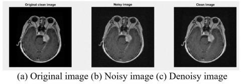
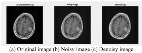
In this section, three image samples were used to illustrate the noise removal results as the first preprocessing step (Figure 7-9).
Figure 7. NLM filter results with Gaussian noise standard deviation 5
Figure 8. NLM filter results with Gaussian noise standard deviation 5
Figure 9. NLM filter results with Gaussian noise standard deviation 5
As can be seen in Figures 7-9, the image quality was improved after noise removal.
Also, despite noise removal, the edges still have more detail than other noise removal methods.
Among the advantages of these non-local filters are the desired quality and quantitative results in a variety of images, especially textured and duplicate ones. That's why we've tried to use this method for pre-processing to help improve noise elimination. Table 3 examines the quantitative criteria for noise abatement.
Table 3. Results of NLM filter quantification criteria in the proposed method
|
Sigma |
PSNR1 |
PSNR2 |
SSIM1 |
SSIM2 |
MSE1 |
MSE2 |
|
σ=5 |
37.21 |
43.92 |
0.87 |
0.95 |
0.12 |
0.02 |
|
σ=10 |
34.25 |
41.92 |
0.65 |
0.94 |
0.18 |
0.05 |
|
σ=15 |
28.21 |
37.55 |
0.61 |
0.92 |
0.24 |
0.12 |
4.3.2 ROI results in the proposed method
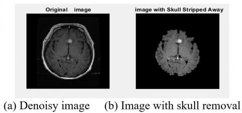
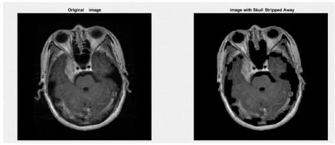
The second step of pre-processing was to remove the skulls of the extra areas. This was used to increase the speed and accuracy of segmentation detection. The skull removal results have been shown in Figures 10 and 11.
Figure 10. Skull removal results
Figure 11. Skull removal results
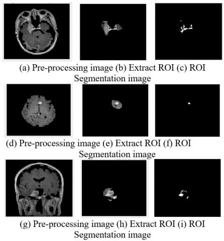
4.3.3 ROI results in the proposed method
Figure 12. ROI Segmentation results
The images were recovered after the pre-processing noise removal and skull removal. Finally, the area of interest (ROI) in MRI images was examined to identify the tumor area in Figure 12.
After presenting the ROI results, the following section compares the segmentation of the proposed method, i.e. the similarity of the proposed binary segmentation with the actual segmentation in Figure 13. Then, the proposed method is evaluated with two criteria, IOU and DSS, with the spectral clustering method in Table 4. It should be noted that the IOU and DSS index criteria are considered to be average for all datasets.
Figure 13. The results’ prediction of the Proposed Method
As can be seen from Figure 13, the proposed method performs much better than the method presented by Angulakshmi and Priya [11], and Table 4 compares the IOU and DSS criteria.
Table 4. Results of Dice score criteria in the proposed method with other methods
|
Methods |
High-grade (real) |
Low-grade (real) |
High-grade (synth) |
Low-grade (synth) |
||||
|
Edema |
TC |
Edema |
TC |
Edema |
TC |
Edema |
TC |
|
|
Classification forest [21] |
0.48 |
0.79 |
0.42 |
0.61 |
0.51 |
0.28 |
0.26 |
0.33 |
|
Tumor cut [22] |
0.58 |
0.80 |
0.55 |
0.69 |
0.56 |
0.32 |
0.27 |
0.35 |
|
spectral clustering [11] |
0.87 |
0.92 |
0.76 |
0.86 |
0.72 |
0.58 |
0.35 |
0.58 |
|
Proposed |
0.89 |
0.95 |
0.81 |
0.88 |
0.75 |
0.63 |
0.42 |
0.61 |
|
Methods |
High-grade (real) |
Low-grade (real) |
High-grade (synth) |
Low-grade (synth) |
||||
|
Edema |
TC |
Edema |
TC |
Edema |
TC |
Edema |
TC |
|
|
Spectral [11] clustering |
0.85 |
0.90 |
0.83 |
0.85 |
0.74 |
0.62 |
0.41 |
0.63 |
|
Proposed |
0.88 |
0.93 |
0.85 |
0.89 |
0.77 |
0.65 |
0.43 |
0.64 |
4.4 Comparison of ROI results of the proposed method with other methods
Now, after examining the ROI segmentation quality, the proposed method will be compared with spectral clustering [11], KASP [16], and Nystrom [17].
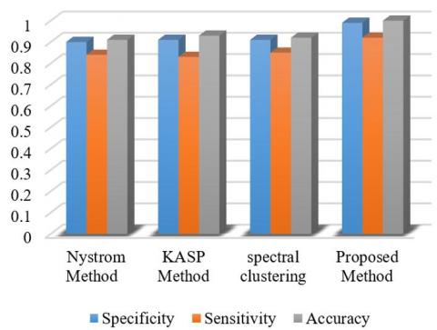
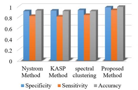
There are three types of tumors in the images: meningioma, glioma, and pituitary, which, in Figure 14, their Specificity, Sensitivity, and Accuracy of different methods for meningioma images have been compared. Based on Figure 14, the proposed method performs better than other methods in terms of specificity criteria, sensitivity, and accuracy. Spectral clustering method is significantly ranked second. Other KASP and Nystrom methods are next in order.
The performance of the proposed method with different methods for glioma and pituitary brain tumor images are illustrated in Figures 15 and 16.
According to Figures 15 and 16, the proposed method is quite superior to the other methods. Based on Figure 16, the sensitivity diagram in other methods has poor performance compared to the proposed method.
In the segmentation method, using the Nystrom method, the similar matrix is not used for spectral clustering, and they randomly select pixel points from the given origin. The KASP method uses the K-means cluster center to express the similarity matrix. For this reason, both methods are less accurate and have a lower computational load than the proposed method. The spectral clustering method, based on super pixels, has a lower computational load for spectral clustering and is more accurate due to the similarity matrix based on super pixels.
Tables 6-8 show the quantitative criteria of the proposed method compared to other methods.
Figure 14. Comparison of different methods of meningioma images
Figure 15. Comparison of different methods of glioma images
Figure 16. Comparison of different methods of pituitary images
Figure 17. Comparison of different methods of pituitary images
Figure 18. Comparison of different methods of pituitary images
Figure 19. Comparison of different methods of pituitary images
Table 6. Comparison of quantitative criteria for different methods of meningioma images
|
Methods |
Accuracy |
Sensitivity |
Specificity |
|
Method [17] Nystrom |
0.91 |
0.90 |
0.84 |
|
Method [16] KASP |
0.93 |
0.91 |
0.83 |
|
Spectral Clustering Method [11] |
0.93 |
0.91 |
0.85 |
|
Proposed Method |
1 |
0.99 |
0.92 |
Table 7. Comparison of quantitative criteria for different methods of glioma images
|
Methods |
Accuracy |
Sensitivity |
Specificity |
|
Method [17] Nystrom |
0.91 |
0.82 |
0.92 |
|
Method [16] KASP |
0.92 |
0.81 |
0.91 |
|
Spectral Clustering Method [11] |
0.93 |
0.84 |
0.91 |
|
Proposed Method |
0.98 |
0.93 |
0.99 |
Table 8. Comparison of quantitative criteria for different methods of pituitary images
|
Methods |
Accuracy |
Sensitivity |
Specificity |
|
Method [17] Nystrom |
0.85 |
0.83 |
0.9 |
|
Method [16] KASP |
0.89 |
0.79 |
0.89 |
|
Spectral Clustering Method [11] |
0.90 |
0.84 |
0.91 |
|
Proposed Method |
0.92 |
0.90 |
0.90 |
As shown in Tables 6, 7, and 8, the quantitative criteria of the proposed method are better than other methods.
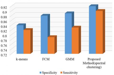
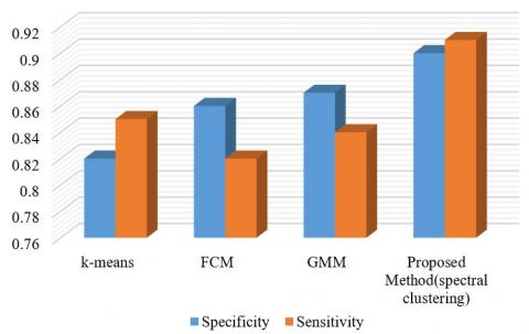
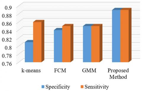
The spectral clustering method in the proposed method is shown along with other K-means, FCM, and GGM clusters in Figures 17-19 meningioma’s, glioma, and pituitary images.
As shown in Figures 17-19, it is weakness clustering in k-means clustering based on Euclidean distance clustering work, except pituitary images in other performance images. In the FCM method, where the outlier’s data problem exists in the early clustering centers, it works closely with the GMM clustering. The spectral clustering method has relatively strong performance in all three image types.
In the present study, the brain tumor detection method in MRI imaging was presented using super pixel-based image processing and clustering techniques. First, the non-local mean algorithm was used for pre-processing. The nonlocal averaging algorithm has so far attracted some attention and popularity by providing acceptable and valuable results in natural images over other noise removal methods. The advantages of this filter are the desirable quantitative and qualitative results in a variety of images, especially texture and duplicate images. At the same time, the algorithm's performance dependence on its parameters, especially the smoothing kernel width (h) and low processing speed, are the most significant drawbacks of this method. For this reason, this method was used for pre-processing to help improve noise removal. Another pre-processing was performed to remove the skull, which eliminates the extra areas and accelerates the segmentation operation. However, the proposed method can distinguish the precise determination of tumor location and size. This method provided a method for segmenting a brain tumor based on a spectral clustering algorithm to improve the detection method using a computer. In addition, it helps to identify tumor-like blocks accurately compared to manual segmentation. Finally, the tumor was extracted from the image, and its exact position and shape were determined.
[1] Pandey, A., Beg, S., Yadav, A. (2016). Image processing technique for the enhancement of brain tumor pattern. Journal of Research and Development in Applied Science and Engineering, 9(2): 1-4.
[2] Borole, Y., Nimbhore, S., Seema, Kawthekar, S. (2015). Image processing techniques for brain tumor detection: A review. Journal of Emerging Trends & Technology in Computer Science (IJETTCS), 4(5(2)): 28-32.
[3] Carlos, A., Sementille, A., Manuel, J. (2019). Techniques of medical image processing and analysis accelerated by high-performance computing: A systematic literature review. Journal of Real-Time Image Processing, 16(6): 1891-1908. https://doi.org/10.1007/s11554-017-0734-z
[4] Demirhan A., Toru M., Guler, I. (2015). Segmentation of tumor and edema along with healthy tissues of brain using wavelets and neural networks. Journal of Biomedical and Health Informatics, 19(4): 1451-1458. https://doi.org/10.1109/JBHI.2014.2360515
[5] Alqudah, A.M., Alquraan, H., Qasmieh, I.A., Alqudah, A., Al-Sharu, W. (2020). Brain tumor classification using deep learning technique--A comparison between cropped, uncropped, and segmented lesion images with different sizes. Image and Video Processing (eess. IV), 8(6): 3684-3691. https://doi.org/10.30534/ijatcse/2019/155862019
[6] Rajan, P., Sundar, C. (2019). Brain tumor detection and segmentation by intensity adjustment. Journal of Medical Systems, 43(8): 282. https://doi.org/10.1007/s10916-019-1368-4
[7] Usha, R., Perumal, K. (2019). SVM classification of brain images from MRI scans using morphological transformation and GLCM texture features. International Journal of Computational Systems Engineering, 5(1): 18-23. https://doi.org/10.1504/IJCSYSE.2019.098415
[8] Menze, B.H., Jakab, A., Bauer, S., Kalpathy-Cramer, J., Farahani, K., Kirby, J., Lanczi, L. (2014). The multimodal brain tumor image segmentation benchmark (BRATS). IEEE Transactions on Medical Imaging, 34(10): 1993-2024. https://doi.org/10.1109/TMI.2014.2377694
[9] Su, P., Jinhua, Y., Li, H., Chi, L., Xue Z. (2013). Superpixel-based segmentation of glioblastoma multiforme from multimodal MR images. International Workshop on Multimodal Brain Image Analysis, pp. 74-83. https://doi.org/10.1007/978-3-319-02126-3_8
[10] Sauwen, N., Acou, M., Van Cauter, S., Sima, D.M., Veraart, J., Maes, F., Van Huffel, S. (2016). Comparison of unsupervised classification methods for brain tumor segmentation using multi-parametric MRI. NeuroImage: Clinical, 12: 753-764. https://doi.org/10.1016/j.nicl.2016.09.021
[11] Angulakshmi, M., Priya, L. (2018). Brain tumour segmentation from MRI using superpixels based spectral clustering. Journal of King Saud University - Computer and Information Sciences, 1-12. https://doi.org/10.1016/j.jksuci.2018.01.009
[12] Foi, A., Boracchi, G. (2016). Foveated nonlocal self-similarity. International Journal of Computer Vision, 1-32. https://doi.org/10.1007/s11263-016-0898-1
[13] Manjón, J.V., Coupé, P., Buades, A. (2015). MRI noise estimation and denoising using non-local PCA. Medical Image Analysis, 22(1): 35-47. https://doi.org/10.1016/j.media.2015.01.004
[14] Hsu, H.C., Wang, M.S. (2012). Detection of copy-move forgery image using Gabor descriptor. Anti-Counterfeiting, Security, and Identification, pp. 1-4. https://doi.org/10.1109/ICASID.2012.6325319
[15] Huang, Y., Lu, W., Sun, W., Long, D. (2011). Improved DCT-based detection of copy-move forgery in images. Forensic Science International, 206(1-3): 178-184. https://doi.org/10.1016/j.forsciint.2010.08.001
[16] Zikic, D., Glocker, B., Konukoglu, E., Shotton, J., Criminisi, A., Ye, D., Price, S.J. (2012). Context-sensitive classification forests for segmentation of brain tumor tissues. In Proc. MICCAI-BRATS, pp. 22-30.
[17] Fowlkes, C., Belongie, S., Chung, F., Malik, J. (2004). Spectral grouping using the Nystrom method. IEEE Transactions on Pattern Analysis and Machine Intelligence, 26(2): 214-225. https://doi.org/10.1109/TPAMI.2004.1262185
[18] Hossin, M., Sulaiman, M.N. (2015). A review on evaluation metrics for data classification evaluations. International Journal of Data Mining & Knowledge Management Process, 5(2): 1-11.
[19] Zhang, L., Dong, W., Zhang, D., Shi, G. (2010). Two-stage image denoising by principal component analysis with local pixel grouping. Pattern Recognition, 43(4): 1531-1549. https://doi.org/10.1016/j.patcog.2009.09.023b
[20] Ndajah, P., Kikuchi, H., Yukawa, M., Watanabe, H., Muramatsu, S. (2010). SSIM image quality metric for denoised images. In Proc. 3rd WSEAS Int. Conf. on Visualization, Imaging and Simulation, pp. 53-58.
[21] Zikic, D., Glocker, B., Konukoglu, E., Shotton, J., Criminisi, A., Ye, D., Demiralp, C., Thomas, O.M., Das, T., Jena, R., Price, S.J. (2012). Context-sensitive classification forests for segmentation of brain tumor tissues. In Proc. MICCAI-BRATS, pp. 22-30.
[22] Hamamci, A., Unal, G. (2012). Multimodal brain tumor segmentation using the tumor-cut method on the BraTS dataset. Proc. MICCAI-BRATS, pp. 19-23.