Maumita Das* | Roshan Kumar | Bikas Chandra Sahana
© 2020 IIETA. This article is published by IIETA and is licensed under the CC BY 4.0 license (http://creativecommons.org/licenses/by/4.0/).
OPEN ACCESS
The primary objective of this research paper, is to introduce an effective hybrid window function for low pass finite impulse response (FIR) filter design which is useful for denoising the electrocardiogram (ECG) signals corrupted by additive white gaussian noise (AWGN) even at low signal to noise ratio (SNR) condition. The noise may be introduced during ambulatory patient monitoring in wireless ECG recording environment. For proper diagnosis, it is very essential to receive noiseless signal even at very low SNR. To reach this objective, a hybrid window function is proposed and a linear phase FIR low pass filter is designed by using the proposed windowing technique. The proposed hybrid window is a product of Blackman and flattop window functions with modified window coefficients. Stopband attenuation of the filter constructed using proposed hybrid window is very high with respect to other traditional window functions and different hybrid window functions created by different combinations of some well-known traditional windows. Filter designed with the proposed hybrid window function have comparable transition bandwidth with respect to other hybrid window functions. ECG denoising performance of the proposed filter is better with respect to others in low SNR environment.
additive white gaussian noise, electrocardiogram denoising, finite impulse response low pass filter, window functions
Filter is a key component in entire communication system and signal processing. In digital signal processing, the impulse response of a FIR (Finite impulse response) filter and an IIR (Infinite impulse response) filter have a finite and infinite number of samples accordingly as their name suggests [1]. In FIR filter impulse response settles to zero in finite time. The linear phase characteristics i.e. not to distort the phase of the signal, makes FIR filters much more useful in many industries. IIR filters can be used if the linear phase is not a concern. Also, IIR filters are beneficial as they require low filter order and less computation as compared to FIR. FIR filters are used almost everywhere for its stability due to the absence of feedback. In the adaptive filter design, FIR is the best choice [2]. The application of FIR filter involves linear interpolation, linear predictive coding, spatial beamforming, adaptive filters, speech analysis, speech modeling and multirate signal processing. Various approaches like, frequency sampling method, windowing techniques, Parks – McClellan method and equiripple FIR filter design using the FFT algorithm can be used in FIR filter design. The windowing technique is used to achieve the coefficients of the desired filter. Window design function has more advantage over other filter design techniques in terms of simplicity, robustness and good performance.
The ECG signal is the measure of the electrical activity of the cardiac muscle [3]. It is considered as a non-stationary signal. In the past few years, the proper diagnosis of ECG signal becomes a challenging phenomenon. The ECG signal is a very sensitive signal to the noise due to the low-frequency band (0.5Hz-150Hz) and suffers various kind of internal and external interference [4]. Internal interferences include the fluctuation of human organs on the ECG signals. During the recording process of the ECG signal, the external noises due to electrodes and the influence of the power line frequency are under this category. Also now a days, with the advancement of different communication systems like mobile and satellite communication, telemedicine has becomes very popular techniques for remote medical care where diagnosis by the specialist is most essential before applying medicine to the unreachable patient [5]. In the context of wireless communication, the ECG recording mechanism is widely used. Overcoming the detrimental effect of additive white gaussian noise becomes a big challenge. Therefore, an efficient filtering technique is required for the denoising of the ECG signal.
An efficient algorithm based on three steps to denoising ECG signals, using the adaptive dual threshold filter (ADTF) and the discrete wavelet transform (DWT) was proposed by Jenkal et al. [4]. Some simulated figures were presented for qualitative analysis and some parameters like MSE, RMSE, PRD, etc. were measured to give a proper comparison for quantitative analysis. A new alternative algorithm was presented by Ercelebi [5] for the reduction of noise in ECG signals using a lifting-based discrete wavelet transform and level-dependent threshold estimator for ECG signals corrupted with muscle artifact, electrode motion artifact, and Gaussian noise. The performance of different kind of digital FIR and IIR notch filter for E.C.G signal analysis was showed by Khaing and Naing [6]. FIR low pass, high pass and notch filter using a rectangular window was designed by Chavan et al. [7]. A study was carried out on the performance of those filters by applying the E.C.G signals as an input. An attempt was made to remove the high-frequency components, power line interferences and reduce the baseline drift of E.C.G. signals. Results were compared with the response of the filters designed using other window techniques. The power line interference, motion artifacts, base line drift and instrumental noise of E.C.G signals was analysed which can be filtered out by using elliptic digital filter [8]. Comparison with Butterworth, Chebyshev type I & type II gives good performance of the proposed filter with few limitations. Three filters like high pass, low pass, and notch filter was designed which is applied on E.C.G signal. In 1978, Fredric J. Harris discussed about some well-known and some not well-known window functions in his article. Author shows some different kinds of window functions which are constructed by products, sums, sections, or convolutions of conventional windows. The paper presented Hanning-poisson window which is nothing but the product of Hanning and Poisson windows [9]. Corrected plot of Harris windows was presented by A. Nuttall in 1981. Few new windows with very good sidelobes and optimal behaviour under several different constraints were introduced by him [10]. Then, in 2014, Vivek Kumar et al. proposed a new window function which is the product of hamming and gaussian window. It was claimed that the proposed window is quasi-tunable window with -61.7dB first side lobe magnitude and have main lobe width is 0.210937π [11]. Similar kind of work motivated us to design such filter and we can see that proposed window function provides very less side lobe magnitude.
The paper is organized as follows: Section 2 contains, design of a linear phase FIR filter using the windowing technique is discussed. Theoretical knowledge of different standard window functions is elaborated in section 3. The complete description of the proposed hybrid window function is presented in section 4. The performance comparison of the proposed hybrid window with several other windows is listed in section 5. A comparative study on the magnitude spectrum of the FIR low pass filter design using proposed window function and the other window technique discussed in section 6. Section 7 covers the performance of the FIR filter designed by proposed window function for the noisy ECG signal. All the results of the experiments and discussions are presented in this section. Finally, conclusion is presented in section 8.
To design a causal ideal low pass filter with cutoff frequency $\omega_{c},$ consider Eq. (1) as the desired frequency response $H_{d}\left(e^{j \omega}\right)$[10]
$H_{d}\left(e^{j \omega}\right)=\left\{\begin{array}{ll}1, & | \phi \leq \omega \\ 0, & \omega<| \phi \leq \pi\end{array}\right.$ (1)
In the design of digital filters, the major interest is in the amplitude response of the filter only and therefore, by using the Fourier series expansion method we can easily calculate the impulse response of the desired FIR filter.
$h_{d}(n)=\left\{\begin{array}{ll}\frac{\omega_{c}}{\pi}, & n=0 \\ \frac{\omega_{c}}{\pi} \frac{\sin \omega_{c} n}{\omega_{c} n}, & n \neq 0\end{array}\right.$ (2)
To obtain the finite duration impulse response $h(n)$ from the infinite duration impulse response $h_{d}(n),$ we need to multiply $h_{d}(n)$ with the finite duration weighting function $\omega(n) .$ This finite duration weighting function is also known as window function which is used to modify the impulse response of the FIR filters in order to reduce the ripples in the passband and stopband and also achieve the desired transition from passband to stopband. Let the desired filter order be $\ell$ and the Fourier transform of the window function $\omega(n)$ is $\omega\left(e^{j \omega}\right)$
Therefore, the impulse response of the FIR filter will be
$h(n)=h_{d}(n) \times \omega(n)$ (3)
The major effects of windowing are
Thus for windowing, smaller main beam width and the small ripple ratio (i.e. good side beam rejection) are the preferred condition though they are contradictory features to each other. A window function with a decay gradually toward zero has improved side beam attenuation.
In this section, the structure of several commonly used window functions has been discussed [12-15].
3.1 Rectangular window
The weighting function and the spectrum for the $\ell$ -point Rectangular window function is given in Eq. (4) and Eq. (5), respectively.
In time domain,
$\omega_{R}(n)=\left\{\begin{array}{l}1 ; \text { for } \frac{-(\ell-1)}{2} \leq|n| \leq \frac{\ell-1}{2} \\ 0 ; \text { otherw ise }\end{array}\right.$ (4)
In frequency domain,
$\omega_{R}\left(e^{j \omega}\right)=\frac{\sin \left(\frac{\omega \ell}{2}\right)}{\sin \frac{\omega}{2}}$ (5)
3.2 Raised cosine window
The Raised cosine windows are smoother at the end and broader but closer to one at the middle. This kind of structure produces less distortion of $h_{d}(n)$ around $n=0 .$ The $\ell$ -point causal raised cosine window $\omega_{R C}(n)$ is defined as,
$\omega_{R C}(n)=\left\{\begin{array}{ll}a-(1-a) \cos \left(\frac{2 \pi n}{\ell-1}\right) ; & \text { for } n=0 \text { to } \ell-1 \\ 0 & ; \text { for other } n\end{array}\right.$ (6)
The frequency spectrum of the raised cosine window $\omega_{R C}\left(e^{j \omega}\right)$ is obtained by taking Fourier Transform of $\omega_{R C}(n)$ and is expressed as,
$\omega_{R C}\left(e^{j \omega}\right)=a \frac{\sin \frac{\omega \ell}{2}}{\sin \frac{\omega}{2}}+\frac{1-a}{2} \frac{\sin \left(\frac{\omega \ell}{2}-\frac{\pi \ell}{\ell-1}\right)}{\sin \left(\frac{\omega}{2}-\frac{\pi}{\ell-1}\right)}+\frac{1-a}{2} \frac{\sin \left(\frac{\omega \ell}{2}+\frac{\pi \ell}{L-1}\right)}{\sin \left(\frac{\omega}{2}+\frac{\pi}{\ell-1}\right)}$ (7)
3.2.1 Hanning window
Hanning window is the type of raised cosine window. It is obtained by putting a=0.5 in Eq. (6). Thus the causal Hanning window $\omega_{R C}(n)$ is defined as,
$\omega_{H a n n}(n)=\left\{\begin{array}{ll}0.5-0.5 \cos \left(\frac{2 \pi n}{\ell-1}\right) & ; \text { for } n=0 \text { to } \ell-1 \\ 0 & ; \text { for other } n\end{array}\right.$ (8)
The frequency response of Hanning window is also obtained by putting a=0.5 in Eq. (7).
${{\omega }_{Hann}}\left( {{e}^{j\omega }} \right)=0.5\frac{\sin \frac{\omega \ell }{2}}{\sin \frac{\omega }{2}}+0.25\frac{\sin \left( \frac{\omega \ell }{2}-\frac{\pi \ell }{\ell -1} \right)}{\sin \left( \frac{\omega }{2}-\frac{\pi }{\ell -1} \right)}+0.25\frac{\sin \left( \frac{\omega \ell }{2}+\frac{\pi \ell }{\ell -1} \right)}{\sin \left( \frac{\omega }{2}+\frac{\pi }{\ell -1} \right)}$ (9)
3.2.2 Hamming window
Hamming Window is also derived from the raised cosine window by keeping a=0.54. Its window coefficients adjusted, so as to achieve lower sidebeam peak compared to Hanning window [16].
In the time domain
${{\omega }_{Hamm}}\left( n \right)=\left\{ \begin{align} & 0.54-0.46\cos \left( \frac{2\pi n}{\ell -1} \right)\,\,\,;\,\,\,\,\,\,\,for\,\,n=0\,\,to\,\,\ell -1 \\ & 0\,\,\,\,\,\,\,\,\,\,\,\,\,\,\,\,\,\,\,\,\,\,\,\,\,\,\,\,\,\,\,\,\,\,\,\,\,\,\,\,\,\,\,\,\,;\,\,\,\,\,\,for\,\,other\,\,n \\\end{align} \right.$ (10)
In the frequency domain
${{\omega }_{Hamm}}\left( {{e}^{j\omega }} \right)=0.54\frac{\sin \frac{\omega \ell }{2}}{\sin \frac{\omega }{2}}+0.23\frac{\sin \left( \frac{\omega \ell }{2}-\frac{\pi \ell }{\ell -1} \right)}{\sin \left( \frac{\omega }{2}-\frac{\pi }{\ell -1} \right)}+0.23\frac{\sin \left( \frac{\omega \ell }{2}+\frac{\pi \ell }{\ell -1} \right)}{\sin \left( \frac{\omega }{2}+\frac{\pi }{\ell -1} \right)}\,\,\,\,$ (11)
3.3 Kaiser window
The main beam width and the side beams attenuation are controlled separately in Kaiser window [17].
In time domain $\ell$-point Kaiser window is given as
$\omega_{k a}(n)=\left\{\begin{array}{l}\frac{I_{0}(b)}{I_{0}(a)} ; \text { for } \frac{-(\ell-1)}{2} \leq|n| \leq \frac{\ell-1}{2} \\ 0 ; \quad \text { otherwise }\end{array}\right.$ (12)
where,
$b=a\left[1-\left(\frac{2 n}{\ell-1}\right)^{2}\right]^{0.5} ; I_{0}(k)=1+\sum_{m=1}^{\infty}\left[\frac{1}{m !}\left(\frac{k}{2}\right)^{m}\right]^{2}$
$I_{0}(k)=ModifiedBasselfunction$
$a=Tunningparameter $
3.4 Blackman window
It is a window of cosine series. $\ell$-point Blackman window defined in the time domain as
$\omega_{B}(n)=\left\{\begin{array}{l}0.42-0.5 \cos \left(\frac{2 \pi n}{\ell-1}\right)+0.08 \cos \left(\frac{4 \pi n}{\ell-1}\right) ; \text { for } n=0 \text { to } \ell-1 \\ 0\end{array} \text { ; for other } n\right.$ (13)
In the frequency domain
$\omega_{B}\left(e^{j \sigma}\right)=0.42 \frac{\sin \frac{\omega \ell}{2}}{\sin \frac{\omega}{2}}+0.25 \frac{\sin \left(\frac{\omega \ell}{2}-\frac{\pi \ell}{\ell-1}\right)}{\sin \left(\frac{\omega}{2}-\frac{\pi}{\ell-1}\right)}+0.25 \frac{\sin \left(\frac{\omega \ell}{2}+\frac{\pi \ell}{\ell-1}\right)}{\sin \left(\frac{\omega}{2}+\frac{\pi}{\ell-1}\right)}+0.04 \frac{\sin \left(\frac{\omega \ell}{2}-\frac{2 \pi \ell}{\ell-1}\right)}{\sin \left(\frac{\omega}{2}-\frac{2 \pi}{\ell-1}\right)}+0.04 \frac{\sin \left(\frac{\omega \ell}{2}+\frac{2 \pi \ell}{\ell-1}\right)}{\sin \left(\frac{\omega}{2}+\frac{2 \pi}{\ell-1}\right)}$ (14)
3.5 Flattop window
A flat top window provides minimal scalloping loss that relates to the flatness of the main lobe in the frequency domain. It is a partially negative-valued window.
In time domain the flattop window is defined as,
$\omega_{F}(n)=\delta_{0}-\delta_{1} \cos (\Psi)+\delta_{2} \cos (2 \Psi)-\delta_{3} \cos (3 \Psi)+\delta_{4} \cos (4 \Psi)$ (15)
where,
$\Psi=\frac{(2 n \pi)}{(\ell-1)}$
$\ell=Orderofthefilter$, $0 \leq n \leq \ell-1$
$\delta_{0}=0.21557896_{1}=0.4166316$
$\delta_{2}=0.27726316 \delta_{3}=0.08357895$
$\delta_{4}=0.00694737$
In frequency domain,
$\omega_{F}\left(e^{j \omega}\right)=0.21557895 \frac{\sin \frac{\omega \ell}{2}}{\sin \frac{\omega}{2}}+0.21 \frac{\sin \left(\frac{\omega \ell}{2}-\frac{\pi \ell}{\ell-1}\right)}{\sin \left(\frac{\omega}{2}-\frac{\pi}{\ell-1}\right)}+0.21 \frac{\sin \left(\frac{\omega \ell}{2}+\frac{\pi t}{\ell-1}\right)}{\sin \left(\frac{\omega}{2}+\frac{\pi}{\ell-1}\right)}+0.14 \frac{\sin \left(\frac{\omega}{2}-\frac{2 \pi \ell}{\ell-1}\right)}{\sin \left(\frac{\omega}{2}-\frac{2 \pi}{\ell-1}\right)}+0.14 \frac{\sin \left(\frac{\omega \ell}{2}+\frac{2 \pi \ell}{\ell-1}\right)}{\sin \left(\frac{\omega}{2}+\frac{2 \pi}{\ell-1}\right)}$
$+0.04 \frac{\sin \left(\frac{\omega \ell}{2}-\frac{3 \pi}{\ell-1}\right)}{\sin \left(\frac{\omega}{2}-\frac{\pi}{\ell-1}\right)}+0.04 \frac{\sin \left(\frac{\omega \ell}{2}+\frac{3 \pi \ell}{\ell-1}\right)}{\sin \left(\frac{\omega}{2}+\frac{\pi}{\ell-1}\right)}+0.003 \frac{\sin \left(\frac{\omega \ell}{2}-\frac{4 \pi \ell}{\ell-1}\right)}{\sin \left(\frac{\omega}{2}-\frac{2 \pi}{\ell-1}\right)}+0.003 \frac{\sin \left(\frac{\omega \ell}{2}+\frac{4 \pi \ell}{\ell-1}\right)}{\sin \left(\frac{\omega}{2}+\frac{2 \pi}{\ell-1}\right)}$ (16)
The proposed hybrid window is based on the Blackman and flattop window. It is a product of Blackman and flattop window.
The proposed window is expressed as given below:
$\omega(n)=\omega_{B}(n) \times \omega_{F}(n)=\sum_{i=0}^{6}\left(\delta_{i} \times \cos (i \times \Psi)\right)$ (17)
where,
$\Psi=\frac{(2 n \pi)}{(l-1)}$
$\ell=$Order of the filter,$\quad 0 \leq n \leq \ell-1$
$\delta_{0}=.20579$, $\delta_{1}=-.3721$, $\delta_{2}=.25903$
$\delta_{3}=-.12282$, $\delta_{4}=.0034903$, $\delta_{5}=-.0050800$, $\delta_{6}=.00027789$
$\omega_{P}\left(e^{j \omega}\right)=0.20579 \frac{\sin \frac{\omega \ell}{2}}{\sin \frac{\omega}{2}}+0.19 \frac{\sin \left(\frac{\omega \ell}{2}-\frac{\pi \ell}{\ell-1}\right)}{\sin \left(\frac{\omega}{2}-\frac{\pi}{\ell-1}\right)}+0.19 \frac{\sin \left(\frac{\omega \ell}{2}+\frac{\pi \ell}{\ell-1}\right)}{\sin \left(\frac{\omega}{2}+\frac{\pi}{\ell-1}\right)}$
$+0.13 \frac{\sin \left(\frac{\omega \ell}{2}-\frac{2 \pi \ell}{\ell-1}\right)}{\sin \left(\frac{\omega}{2}-\frac{2 \pi}{\ell-1}\right)}+0.13 \frac{\sin \left(\frac{\omega \ell}{2}+\frac{2 \pi \ell}{\ell-1}\right)}{\sin \left(\frac{\omega}{2}+\frac{2 \pi}{\ell-1}\right)}+0.06 \frac{\sin \left(\frac{\omega \ell}{2}-\frac{3 \pi \ell}{\ell-1}\right)}{\sin \left(\frac{\omega}{2}-\frac{\pi}{\ell-1}\right)}+0.06 \frac{\sin \left(\frac{\omega \ell}{2}+\frac{3 \pi \ell}{\ell-1}\right)}{\sin \left(\frac{\omega}{2}+\frac{\pi}{\ell-1}\right)}$
$+0.002 \frac{\sin \left(\frac{\omega \ell}{2}-\frac{4 \pi \ell}{\ell-1}\right)}{\sin \left(\frac{\omega}{2}-\frac{2 \pi}{\ell-1}\right)}+0.002 \frac{\sin \left(\frac{\omega \ell}{2}+\frac{4 \pi \ell}{\ell-1}\right)}{\sin \left(\frac{\omega}{2}+\frac{2 \pi}{\ell-1}\right)}+0.003 \frac{\sin \left(\frac{\omega \ell}{2}-\frac{5 \pi \ell}{\ell-1}\right)}{\sin \left(\frac{\omega}{2}-\frac{\pi}{\ell-1}\right)}+0.003 \frac{\sin \left(\frac{\omega \ell}{2}+\frac{5 \pi \ell}{\ell-1}\right)}{\sin \left(\frac{\omega}{2}+\frac{\pi}{\ell-1}\right)}+0.00014 \frac{\sin \left(\frac{\omega \ell}{2}-\frac{6 \pi \ell}{\ell-1}\right)}{\sin \left(\frac{\omega}{2}-\frac{2 \pi}{\ell-1}\right)}+0.00014 \frac{\sin \left(\frac{\omega \ell}{2}+\frac{6 \pi \ell}{\ell-1}\right)}{\sin \left(\frac{\omega}{2}+\frac{2 \pi}{\ell-1}\right)}$ (18)
Figure 1(a) and Figure 1(b), Figure 2(a) and Figure 2(b) & Figure 3(a) and Figure 3(b) shows the time and magnitude response of the blackman window, flattop window and the proposed window function for $\ell$=63 respectively.
Figure 1. Time & Magnitude response of the Blackman window for $\ell$=63
Figure 2. Time & Magnitude response of the flattop window for $\ell$=63
Figure 3. Time & magnitude response of the proposed hybrid window for $\ell$=63
Performance comparison of the proposed hybrid window with several commonly used window functions for window length $\ell$=31 and $\ell$=63 is discussed here. The width of the transition band is directly proportional to the main lobe width and the stopband attenuation is related to the lower value of side lobe ripples in the magnitude response. Therefore, the window function with small main lobe width and decreasing side lobe ripples provides the desired result. Based on this background theory, Table 1 draws a conclusion that though the main beam width is not up to the mark but due to side beam attenuation factor, proposed window function won the battle for any filter length. It can be observed that the magnitude of the first side lobe is -113dB for both $\ell$=31 and $\ell$=63 which is achieved at the expense of increased main lobe width. An improvement of 70.5dB, 81.5dB, 54.9dB, 25.2dB, 99.7dB and 99.3dB for filter length $\ell$=63 are observed relative to hamming, hanning, blackman, flattop, rectangular and kaiser window function respectively. Performance of the proposed window function in stopband attenuation is much better compared to other hybrid window function. Also, the main lobe width or transition bandwidth is decreased by increasing the filter length.
Table 1. Comparative study of properties of different window functions
|
Window Name |
Length of Filter ( $\ell$ ) |
Main Beam Width (-3dB) |
Side Beam Attenuation (dB) |
Leakage Factor |
|
Hamming |
31 |
0.078125 |
-41.7 |
0.04% |
|
Hanning |
31 |
0.085938 |
-31.5 |
0.05% |
|
Blackman |
31 |
0.10938 |
-58.2 |
0% |
|
Flattop |
31 |
0.24219 |
-82.7 |
0% |
|
Rectangular |
31 |
0.054688 |
-13.3 |
9.12% |
|
Kaiser |
31 |
0.054688 |
-13.6 |
8.31% |
|
Blackman-Hamming |
31 |
0.125 |
-72.7 |
0% |
|
Flattop- Hamming |
31 |
0.23438 |
-99.9 |
0% |
|
Hamming- Hanning |
31 |
0.10938 |
-49.7 |
0% |
|
Hanning- Blackman |
31 |
0.125 |
-77.5 |
0% |
|
Hanning- Flattop |
31 |
0.23438 |
-104.9 |
0% |
|
Proposed |
31 |
0.23438 |
-113 |
0% |
|
Hamming |
63 |
0.039063 |
-42.5 |
03% |
|
Hanning |
63 |
0.042969 |
-31.5 |
.05% |
|
Blackman |
63 |
0.050781 |
-58.1 |
0% |
|
Flattop |
63 |
0.11719 |
-87.8 |
0% |
|
Rectangular |
63 |
0.027344 |
-13.3 |
9.15% |
|
Kaiser |
63 |
0.027344 |
-13.7 |
83.36% |
|
Blackman-Hamming |
63 |
0.0625 |
-72.7 |
0% |
|
Flattop- Hamming |
63 |
0.11328 |
-101.8 |
0% |
|
Hamming- Hanning |
63 |
0.054688 |
-49.8 |
0% |
|
Hanning- Blackman |
63 |
0.0625 |
-76.4 |
0% |
|
Hanning- Flattop |
63 |
0.11328 |
-104.9 |
0% |
|
Proposed |
63 |
0.11328 |
-113 |
0% |
(a) Comparison with the traditional windows
(b) Comparison with other combinations of the traditional windows
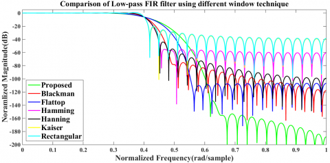
Figure 4. The comparative log-magnitude response of FIR low pass filters using different windowing technique for $\ell$=63
A low pass FIR filter of order $\ell$=63 with cut off frequency $\omega_{c}=0.4 \pi$ has been designed to measure the efficiency of the proposed hybrid window. From the Figure 4(a), it is observed that the low pass FIR filter achieved by using proposed hybrid window offers much lower side lobe peak in comparison to the low pass FIR filter designed using other commonly used window techniques and the side lobe magnitude decreased with frequency.
The comparison result of the proposed hybrid window with other combinations of traditional windows are shown in Figure 4(b). It is clear from the all the comparison results that the proposed filter provides better magnitude response than the others.
For evaluating the performance of the low pass FIR filter with a proposed window function, we pass the ECG signals, added with AWGN noise, through the filter. The filter response is compared with the other standard filter responses [18]. Our main aim to filter out the noise interference from the received noisy signal under any degree of SNR. Actual ECG records, from the MIT-BIH arrhythmia database, are used for our experiments [19]. This database consists of 48 records with a sampling frequency of 360 Hz, i.e. each 360 samples present 1s of the original signal [4].
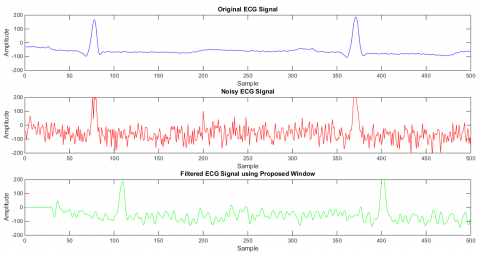
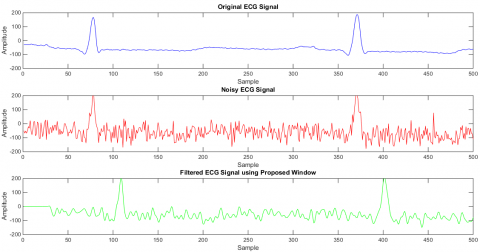
7.1 Qualitative results for E.C.G. denoising
Few figures are taken from the simulation of the proposed method in order to analyze the quality of ECG signal denoising. Qualitative analysis is done on the ECG signal 100 of the MIT-BIH database [19]. The simulation results of the performance of the proposed filter for different additive white Gaussian noise level is shown in the Figure 5 to Figure 8. It is clear from the Figures that the proposed filter retrieved the original ECG signal from any noisy platform, even though at the low SNR where the noise power is superior over the signal power.
The filter performance also analyzed on the basis of total harmonic distortion (THD), SINAD and SNR [3]. THD enumerates the measured total harmonic distortion up to and including the highest harmonic [3]. It is defined as the ratio of the RMS sum of the harmonics to the amplitude of the fundamental tone and it also tells the amount of the distortion of a voltage or current caused due to harmonics in the signal.
Figure 5. Proposed filter response under 1dB SNR
Figure 6. Proposed filter response under 3dB SNR
Figure 7. Proposed filter response under 5dB SNR
Figure 8. Proposed filter response under 10dB SNR
Table 2. Simulated results at different AWGN noise for different LP-FIR filter
|
Window Name |
Input SNR 1dB |
Input SNR 5dB |
Input SNR 10dB |
||||||
|
THD |
SINAD |
SNR |
THD |
SINAD |
SNR |
THD |
SINAD |
SNR |
|
|
Noisy Signal |
-04.42 |
-16.29 |
-15.22 |
2.55 |
-13.28 |
-14.12 |
2.42 |
-11.64 |
-11.39 |
|
Proposed |
-11.30 |
-13.40 |
-12.01 |
1.80 |
-10.88 |
-11.80 |
2.35 |
-10.65 |
-10.28 |
|
Blackman |
-10.92 |
-13.53 |
-12.11 |
1.80 |
-10.96 |
-11.86 |
2.35 |
-10.69 |
-10.34 |
|
Flattop |
-11.24 |
-13.44 |
-12.04 |
1.80 |
-10.90 |
-11.82 |
2.35 |
-10.66 |
-10.30 |
|
Hamming |
-10.82 |
-13.56 |
-12.13 |
1.80 |
-10.98 |
-11.88 |
2.35 |
-10.70 |
-10.35 |
|
Hanning |
-10.79 |
-13.56 |
-12.13 |
1.80 |
-10.98 |
-11.88 |
2.35 |
-10.69 |
-10.35 |
|
Kaiser |
-11.05 |
-13.65 |
-12.13 |
1.84 |
-10.99 |
-11.95 |
2.39 |
-10.75 |
-10.40 |
|
Rectangular |
-11.07 |
-13.66 |
-12.13 |
1.84 |
-10.99 |
-11.96 |
2.39 |
-10.76 |
-10.40 |
THD is a vital aspect in communications, audio and power systems and it should typically be as low as possible (but not always). SINAD calculates the measured signal in noise and distortion [3]. It is used in mobile stations operating on an analog system like Advanced Mobile Phone Service (AMPS), to measure the audio quality of the receiver. It is the ratio of Signal + Noise + Distortion to the Noise + Distortion and expressed in dB. SNR is the measure of useful information and is the ratio of the strength of an electrical or other signal carrying information to that of unwanted interference. It is clear from the Table 2, that with respect to the other standard window function, the proposed hybrid window introduces such a fir filter that gives comparatively low total harmonic distortion, high SINAD, and high SNR.
7.2 Quantitative results of E.C.G. denoising
To evaluate statistically the efficiency of the proposed method following five parameters are calculated [4-5, 20]:
$M S E=\frac{1}{\mathrm{N}} \sum_{m=1}^{N}(y(m)-x(m))^{2}$ (19)
The root means square error
$R M S E=\sqrt{\frac{1}{\mathrm{N}} \sum_{m=1}^{\mathrm{N}}(y(m)-x(m))^{2}}$ (20)
The percent root means square difference
$P R D=100 \times \sqrt{\frac{\sum_{m=1}^{N}(y(m)-x(m))^{2}}{\sum_{m=1}^{l} x^{2}(m)}}$ (21)
The signal-to-noise ratio output [21]
$S N R_{\text {out}}=10 \times \log _{10} \frac{\sum_{m=1}^{\mathrm{N}} x^{2}(m)}{\sum_{m=1}^{\mathrm{N}}(y(m)-x(m))^{2}}$ (22)
The signal-to-noise ratio improvement
$S N R_{i m p}=10 \times \log _{10} \frac{\sum_{m=1}^{N}(\hat{x}(m)-x(m))^{2}}{\sum_{m=1}^{N}(y(m)-x(m))^{2}}$ (23)
where, $x(m)$ is the pure signal, $x(m)$ is the impure signal by the noises, $y(m)$ is the filter output and $N$ is the length of the ECG signal, which is the number of samples of each MIT-BIH signal $[19] .$ Five sets of ECG signal from the MIT-BIH arrhythmia database (MLII) are tested and comparative results with using others windowing for a different level of interference are listed in the Table 3 and Table 4
The percentage of distortion present in the denoised signal is calculated using the expression of PRD exposed in Table 3 The PRD values of the proposed method almost same as we increase the level of input SNR. The largest value of output SNR indicates higher signal strength compare to external interferences which are a desirable feature for the improved performance of the signal denoising. All the comparative results shown in Table 4 are clearly indicating that the proposed algorithm supports the background theory. The MSE is the measure of how actually the predicted values of the filter are different from the original values. It is always non- negative and values closer to zero are better.
Table 3. The MSE, RMSE and PRD values for different filter models tested with various ECG records at different AWGN level
|
MIT- BIH Database |
Window |
MSE |
RMSE |
PRD |
||||||
|
WGN 1dB |
WGN 5dB |
WGN 10dB |
WGN 1dB |
WGN 5dB |
WGN 10dB |
WGN 1dB |
WGN 5dB |
WGN 10dB |
||
|
100 |
Proposed |
4007.65 |
3901.60 |
3605.02 |
63.31 |
62.46 |
60.04 |
85.3268 |
75.2637 |
70.8612 |
|
Blackman |
4074.99 |
3958.96 |
3665.32 |
63.84 |
62.92 |
60.54 |
86.1249 |
75.5631 |
71.0032 |
|
|
Flattop |
4026.14 |
3917.21 |
3621.19 |
63.45 |
62.59 |
60.18 |
85.5368 |
75.3421 |
70.8987 |
|
|
Hamming |
4091.15 |
3973.11 |
3679.58 |
63.96 |
63.03 |
60.66 |
86.3224 |
75.6326 |
71.0292 |
|
|
Hanning |
4090.67 |
3972.78 |
3679.48 |
63.96 |
63.03 |
60.66 |
86.3184 |
75.6380 |
71.0365 |
|
|
Kaiser |
4127.13 |
4003.01 |
3707.01 |
64.24 |
63.27 |
60.89 |
86.7277 |
75.7201 |
71.0177 |
|
|
Rectangular |
4128.61 |
4004.22 |
3708.07 |
64.25 |
63.28 |
60.89 |
86.7436 |
75.7211 |
71.0141 |
|
|
107 |
Proposed |
69300.89 |
68867.17 |
69318.73 |
263.25 |
262.43 |
263.28 |
143.8846 |
138.8967 |
134.4727 |
|
Blackman |
69769.28 |
69675.54 |
69675.54 |
264.14 |
263.96 |
263.96 |
144.3384 |
139.0795 |
134.5406 |
|
|
Flattop |
69416.83 |
68971.59 |
69418.27 |
263.47 |
262.62 |
263.47 |
144.0069 |
138.9469 |
134.4908 |
|
|
Hamming |
69884.93 |
69316.63 |
69750.14 |
264.36 |
263.28 |
264.10 |
144.4351 |
139.1140 |
134.5452 |
|
|
Hanning |
69890.39 |
69322.02 |
69756.53 |
264.37 |
263.29 |
264.11 |
144.4446 |
139.1234 |
134.5573 |
|
|
Kaiser |
70064.11 |
69442.02 |
69839.66 |
264.70 |
263.52 |
264.27 |
144.5327 |
139.1060 |
134.4570 |
|
|
Rectangular |
70067.73 |
69444.20 |
69840.71 |
264.70 |
263.52 |
264.27 |
144.5326 |
139.1017 |
134.4486 |
|
|
115 |
Proposed |
11055.02 |
10784.93 |
10863.94 |
105.14 |
103.85 |
104.23 |
94.0258 |
82.2235 |
76.4773 |
|
Blackman |
11205.93 |
10947.52 |
11024.10 |
105.86 |
104.63 |
105.00 |
94.7418 |
82.5224 |
76.5865 |
|
|
Flattop |
11096.77 |
10827.50 |
10906.10 |
105.34 |
104.06 |
104.43 |
94.2307 |
82.3080 |
76.5064 |
|
|
Hamming |
11240.50 |
10988.56 |
11064.80 |
106.02 |
104.83 |
105.19 |
94.9006 |
82.5838 |
76.6049 |
|
|
Hanning |
11240.34 |
10987.81 |
11064.09 |
106.02 |
104.82 |
105.19 |
94.9021 |
82.5892 |
76.6127 |
|
|
Kaiser |
11305.17 |
11073.96 |
11151.04 |
106.33 |
105.23 |
105.60 |
95.1865 |
82.6490 |
76.5810 |
|
|
Rectangular |
11307.64 |
11077.26 |
11154.34 |
106.34 |
105.25 |
105.61 |
95.1963 |
82.6491 |
76.5767 |
|
|
118 |
Proposed |
24400.51 |
23309.55 |
23540.25 |
156.21 |
152.67 |
153.43 |
74.0892 |
59.6738 |
52.2292 |
|
Blackman |
24920.93 |
23899.95 |
24228.66 |
157.86 |
154.60 |
155.66 |
74.9541 |
60.1004 |
52.3792 |
|
|
Flattop |
24536.50 |
23458.93 |
23706.15 |
156.64 |
153.16 |
153.97 |
74.3454 |
59.7895 |
52.2686 |
|
|
Hamming |
25059.95 |
24050.56 |
24407.82 |
158.30 |
155.08 |
156.23 |
75.1221 |
60.2028 |
52.4155 |
|
|
Hanning |
25055.21 |
24045.51 |
24402.44 |
158.29 |
155.07 |
156.21 |
75.1218 |
60.2022 |
52.4187 |
|
|
Kaiser |
25375.06 |
24366.53 |
24771.00 |
159.30 |
156.10 |
157.39 |
75.4005 |
60.3991 |
52.4715 |
|
|
Rectangular |
25388.24 |
24379.66 |
24785.53 |
159.34 |
156.14 |
157.43 |
75.4122 |
60.4058 |
52.4724 |
|
|
124 |
Proposed |
19994.86 |
18722.80 |
17991.71 |
141.40 |
136.83 |
134.13 |
80.6161 |
67.7101 |
61.3381 |
|
Blackman |
20421.90 |
19096.14 |
18414.32 |
142.91 |
138.19 |
135.70 |
81.3997 |
68.1651 |
61.4485 |
|
|
Flattop |
20108.71 |
18822.21 |
18100.85 |
141.81 |
137.19 |
134.54 |
80.8149 |
67.8270 |
61.3714 |
|
|
Hamming |
20525.89 |
19188.17 |
18523.96 |
143.27 |
138.52 |
136.10 |
81.6030 |
68.2684 |
61.4692 |
|
|
Hanning |
20521.72 |
19185.59 |
18518.59 |
143.25 |
138.51 |
136.08 |
81.5952 |
68.2707 |
61.4731 |
|
|
Kaiser |
20752.38 |
19378.28 |
18773.38 |
144.06 |
139.21 |
137.02 |
82.0509 |
68.4328 |
61.4838 |
|
|
Rectangular |
20761.82 |
19386.01 |
18783.90 |
144.09 |
139.23 |
137.05 |
82.0699 |
68.4377 |
61.4828 |
|
Table 4. The SNRimprovement and SNRoutput values for different filter tested with various ECG records at different AWGN level
|
MIT- BIH Database |
Window |
SNRimprovement (dB) |
SNRout |
||||
|
WGN 1dB |
WGN 5dB |
WGN 10dB |
WGN 1dB |
WGN 5dB |
WGN 10dB |
||
|
100 |
Proposed |
0.4279 |
-2.6665 |
-7.0170 |
1.3518 |
2.4338 |
3.0514 |
|
Blackman |
0.3446 |
-2.7053 |
-7.0319 |
1.2818 |
2.3956 |
3.0329 |
|
|
Flattop |
0.4034 |
-2.6761 |
-7.0215 |
1.3304 |
2.4231 |
3.0466 |
|
|
Hamming |
0.3285 |
-2.7153 |
-7.0345 |
1.2676 |
2.3869 |
3.0291 |
|
|
Hanning |
0.3280 |
-2.7154 |
-7.0352 |
1.2675 |
2.3868 |
3.0284 |
|
|
Kaiser |
0.3036 |
-2.7346 |
-7.0354 |
1.2425 |
2.3703 |
3.0278 |
|
|
Rectangular |
0.3028 |
-2.7352 |
-7.0351 |
1.2415 |
2.3698 |
3.0281 |
|
|
107 |
Proposed |
-4.3183 |
-7.7587 |
-12.4553 |
-3.2701 |
-2.6960 |
-2.5286 |
|
Blackman |
-4.3427 |
-7.7703 |
-12.4599 |
-3.3038 |
-2.7084 |
-2.5321 |
|
|
Flattop |
-4.3249 |
-7.7619 |
-12.4565 |
-3.2787 |
-2.6992 |
-2.5296 |
|
|
Hamming |
-4.3480 |
-7.7725 |
-12.4604 |
-3.3114 |
-2.7109 |
-2.5322 |
|
|
Hanning |
-4.3485 |
-7.7731 |
-12.4612 |
-3.3119 |
-2.7115 |
-2.5330 |
|
|
Kaiser |
-4.3547 |
-7.7717 |
-12.4557 |
-3.3207 |
-2.7110 |
-2.5266 |
|
|
Rectangular |
-4.3548 |
-7.7714 |
-12.4552 |
-3.3208 |
-2.7107 |
-2.5260 |
|
|
115 |
Proposed |
-0.4090 |
-3.1835 |
-7.5833 |
0.9166 |
1.7781 |
2.3717 |
|
Blackman |
-0.4785 |
-3.2179 |
-7.5945 |
0.8501 |
1.7438 |
2.3594 |
|
|
Flattop |
-0.4259 |
-3.1935 |
-7.5864 |
0.8994 |
1.7693 |
2.3682 |
|
|
Hamming |
-0.4964 |
-3.2252 |
-7.5964 |
0.8329 |
1.7359 |
2.3576 |
|
|
Hanning |
-0.4963 |
-3.2255 |
-7.5973 |
0.8331 |
1.7354 |
2.3567 |
|
|
Kaiser |
-0.5298 |
-3.2369 |
-7.5938 |
0.7980 |
1.7249 |
2.3605 |
|
|
Rectangular |
-0.5310 |
-3.2372 |
-7.5934 |
0.7967 |
1.7247 |
2.3610 |
|
|
118
|
Proposed |
2.0948 |
-0.5740 |
-4.4379 |
3.0802 |
4.5855 |
5.5807 |
|
Blackman |
1.9842 |
-0.6371 |
-4.4623 |
2.9629 |
4.5319 |
5.5538 |
|
|
Flattop |
2.0644 |
-0.5909 |
-4.4445 |
3.0472 |
4.5711 |
5.5732 |
|
|
Hamming |
1.9595 |
-0.6510 |
-4.4672 |
2.9365 |
4.5191 |
5.5483 |
|
|
Hanning |
1.9597 |
-0.6512 |
-4.4680 |
2.9374 |
4.5189 |
5.5476 |
|
|
Kaiser |
1.9146 |
-0.6725 |
-4.4711 |
2.8829 |
4.4957 |
5.5425 |
|
|
Rectangular |
1.9127 |
-0.6732 |
-4.4710 |
2.8805 |
4.4949 |
5.5425 |
|
|
124 |
Proposed |
1.2268 |
-1.4371 |
-5.8009 |
2.2338 |
3.4410 |
4.3187 |
|
Blackman |
1.1383 |
-1.4882 |
-5.8198 |
2.1323 |
3.3943 |
4.3008 |
|
|
Flattop |
1.2037 |
-1.4500 |
-5.8061 |
2.2081 |
3.4282 |
4.3142 |
|
|
Hamming |
1.1153 |
-1.5007 |
-5.8236 |
2.1070 |
3.3839 |
4.2968 |
|
|
Hanning |
1.1160 |
-1.5008 |
-5.8242 |
2.1079 |
3.3836 |
4.2962 |
|
|
Kaiser |
1.0641 |
-1.5227 |
-5.8259 |
2.0547 |
3.3676 |
4.2929 |
|
|
Rectangular |
1.0620 |
-1.5234 |
-5.8257 |
2.0525 |
3.3671 |
4.2930 |
|
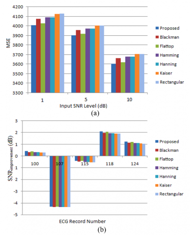
Figure 9. Comparison of MSE (mV) with varying input SNR levels and improvement in SNR with different ECG records for different windowing functions explored in this study
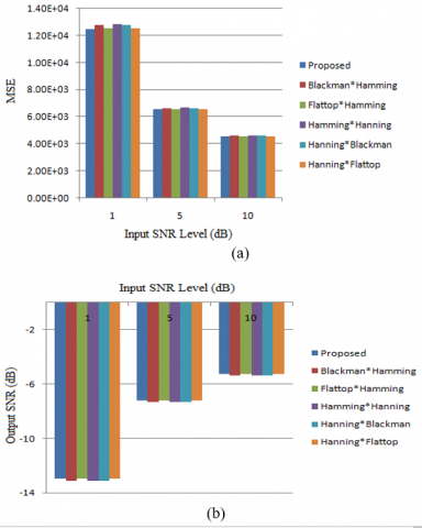
Figure 10. Comparison of MSE(mV) and output SNR(dB) by varying input SNR levels for different hybrid windowing functions
Figure 9(a) and Figure 10(a) shows clearly that the filter response designed with the proposed window provides a comparatively low value of MSE with increasing input SNR level. Analysis is based on ECG signal 100 and 117 of the MIT-BIH database. Comparative graph for different filter shown in Figure 10(b) that output SNR of filter with proposed window combination is better than other filter designed with different combination of traditional window. Figure 9(b) gives SNRimprovent plot for different ECG records in the database at a low level of input SNR and again show the superior performance of the proposed combination against the aforementioned existing approaches.
Comparison results shows better side beam attenuation of the proposed hybrid window function than any other kind of window function. The low pass FIR filter designed with the proposed hybrid window function provides less complexity with comparatively acceptable performance in the application of denoising ECG signals corrupted with AWGN even at low input SNR environment. The cosine coefficient of the proposed window function indicates that the high-order cosine has a very low value coefficient (<<1) which shows that its effect on the window coefficient and filter coefficient can be ignored. The window function can be further improved with fewer cosine terms, therefore, it can reduce the cost in calculation and become a better FIR window function than other window functions.
The authors would like to express the sincerest gratitude to all the reviewers for their useful comments and notes contributing to a noteworthy improvement of this paper.
[1] Oppenheimm, A., Schafer, R., Buck, J. (1999). Discrete-Time Signal Processing. second edition, Prentice-Hall. https://doi.org/10.1007/978-1-4471-0541-1
[2] Proakis, J., Manolakis, D.G. (2007). Digital Signal Processing. fourth edition, Prentice-Hall. https://doi.org/10.2337/diacare.25.10.1802
[3] Goel, S., Kaur, G., Tomar, P. (2015). Performance Analysis of Welch and Blackman Nuttall window for noise reduction of ECG. International Conference on Signal Processing, Computing and Control, Waknaghat, India, pp. 87-91. https://doi.org/10.1109/ISPCC.2015.7375003
[4] Jenkal, W., Latif, R., Toumanari, A., Dliou, A., El B’charri, O., Fadel Maoulainine, M.R. (2016). An efficient algorithm of ECG signal denoising using the adaptive dual threshold filter and the discrete wavelet transform. Biocybernetics And Biomedical Engineering, 36(3): 499-508. https://doi.org/10.1016/j.bbe.2016.04.001
[5] Ercelebi, E. (2003). Electrocardiogram signals de-noising using lifting based discrete wavelet transform. Computers in Biology and Medicine, 34(6): 479-493. https://doi.org/10.1016/S0010-4825(03)00090-8
[6] Khaing, A.S., Naing, Z.M. (2011). Quantitative investigation of digital filters in electrocardiogram with simulated noises. International Journal of Information and Electronics Engineering, 1(3): 210-216. https://doi.org/10.7763/IJIEE.2011.V1. 33
[7] Chavan, M.S., Agarwala, R.A., Uplane, M.D. (2008). Interference reduction in ECG using digital FIR filters based on rectangular window. WSEAS Transactions on Signal Processing, 4(5).
[8] Chavan, M.S., Agarwala, R.A., Uplane, M.D. (2005). Digital elliptic filter application for noise reduction in ECG signal. 4th WSEAS International Conference on Electronics, Control and Signal Processing, Miami, Florida, USA, pp. 58-63.
[9] Harris, F.J. (1978). On the use of windows for harmonic analysis with the discrete fourier transform. Proceedings of the IEEE, 66(1): 51-83. https://doi.org/10.1109/PROC.1978.10837
[10] Nuttall, A. (1981). Some windows with very good sidelobe behavior. IEEE Transactions on Acoustics, Speech, and Signal Processing, 29(1): 84-91. https://doi.org/10.1109/TASSP.1981.1163506
[11] Kumar, V., Bangar, S., Kumar, S.N., Jit, S. (2014). Design of effective window function for FIR filters. IEEE International Conference on Advances in Engineering & Technology Research (ICAETR -2014), Unnao, pp. 1-5. https://doi.org/10.1109/ICAETR.2014.7012964
[12] Mottaghi-Kashtiban, M., Shayesteh, M.G. (2010). A new window function for signal spectrum analysis and FIR filter design. 18th Iranian Conference on Electrical Engineering, Isfahan, pp. 215-219. https://doi.org/10.1109/IRANIANCEE.2010.5507073
[13] Podder, P., Khan, T.Z., Khan, M.H., Rahman, M.M. (2014). Comparative performance analysis of Hamming, Hanning and Blackman window. International Journal of Computer Applications, 96(18): 1-7. https://doi.org/10.5120/16891-6927
[14] Patil, A.M. (2015). A new window function for fir filter design and spectral analysis. International Journal of Advance Research in Science and Engineering, 4(9): 184-194.
[15] Mandloi, M.S., Kumrey, G.R. (2017). FIR high pass filter for improving performance characteristics of various windows. International Journal of Advanced Engineering Research and Science (IJAERS), 4(1): 98-104. https://doi.org/10.22161/ijaers.4.1.15
[16] Shil, M., Rakshit, H., Ullah, H. (2017). An adjustable window function to design an FIR filter. IEEE International Conference on Imagining, Vision & Pattern Recognition (icIVPR). https://doi.org/10.1109/ICIVPR.2017.7890865
[17] Nouri, M., Aghdam, S.A., Aghdam, S.A. (2011). Communication in computer and information science. Analysis of Novel Window Based on the Polynomial Functions, 250: 50-54. https://doi.org/10.1007/978-3-642-25734-6_8
[18] Sun, Y., Chan, K.L., Krishnan, S.M. (2002). ECG signal conditioning by morphological filtering. Computers in Biology and Medicine, 32(6): 465-479. https://doi.org/10.1016/S0010-4825(02)00034-3
[19] Moody, G.B., Mark, R.G. (2001). The impact of the MIT-BIH arrhythmia database. IEEE Engineering in Medicine and Biology Magazine, 20(3): 45-50. http://doi.org/10.1109/51.932724
[20] Wang, J.H., Ye, Y.Q., Pan, X., Gao, X.D. (2015). Parallel-type fractional zero-phase filtering for ECG signal denoising. Biomedical Signal Processing and Control, 18: 36-41. https://doi.org/10.1016/j.bspc.2014.10.012
[21] Zhu, Y.L., Xu, C.G., Xiao, D.G. (2019). Denoising Ultrasonic echo signals with generalized S transform and singular value. Traitement du Signal, 36(2): 139-145. http://doi.org/10.18280/ts.360203