Semiye Demircan* | Humar Kahramanlı Örnek
© 2020 IIETA. This article is published by IIETA and is licensed under the CC BY 4.0 license (http://creativecommons.org/licenses/by/4.0/).
OPEN ACCESS
In the present paper, an approach was developed for emotion recognition from speech data using deep learning algorithms, a problem that has gained importance in recent years. Feature extraction manually and feature selection steps were more important in traditional methods for speech emotion recognition. In spite of this, deep learning algorithms were applied to data without any data reduction. The study implemented the triple emotion groups of EmoDB emotion data: Boredom, Neutral, and Sadness-BNS; and Anger, Happiness, and Fear-AHF. Firstly, the spectrogram images resulting from the signal data after pre-processing were classified using AlexNET. Secondly, the results formed from the Mel-Frequency Cepstrum Coefficients (MFCC) extracted by feature extraction methods to Deep Neural Networks (DNN) were compared. The importance and necessity of using manual feature extraction in deep learning was investigated, which remains a very important part of emotion recognition. The experimental results show that emotion recognition through the implementation of the AlexNet architecture to the spectrogram images was more discriminative than that through the implementation of DNN to manually extracted features.
speech emotion recognition, Deep Neural Network (DNN), Convolutional Neural Network (CNN), deep learning algorithm, Mel-Frequency Cepstrum Coefficients (MFCC)
From a computer−human interaction perspective, emotion recognition is gradually gaining importance. Emotion recognition is conducted by examining changes in blood volume pulses [1], blood pressure [2], facial mimics and gestures [3-5], and brain waves [6], in addition to analyzing speech data [7-9].
Analysis of speech data has significance in the diagnosis of certain human diseases and psychological statuses. Evaluation of the acoustic characteristics of the speech of individuals with depression and a tendency to commit suicide can indicate clues regarding diagnosis [10]. It is also possible to highlight driver errors and ensure more secure driving by following the emotional status of the drivers via the implementation of emotion recognition methods [11]. As the number of calls to emergency call centers increases, it is possible to detect more important calls using emotion recognition [12].
Deep learning is a class of machine learning that employs numerous layers of non-linear operating units for feature extraction and transformation. Each layer considers the output of the previous layer as its input [13]. In terms of Artificial Neural Networks (ANN), the expression of deep learning was first introduced by Aizenberg et al. in 2000 [14]. Subsequently, Hinton et al. 2006 showed how a multilayer feed-forward neural network effectively trains a layer at each iteration, making it possible to conduct fine-tuning via the method of controlled backpropagation [15]. Deep learning architectures perform hierarchical feature extraction that represents the data better than manually extracted features [16].
Deep learning algorithms have been employed to solve problems in many fields such as image and video processing [17], natural language processing [18], biomedical signal and image processing [19, 20], rough sets [21], and speech analysis [22, 23].
Zhang et al. [23] aimed to bridge the affective gap in obtaining emotion from speech signals by utilizing a Deep Convolutional Neural Network (DCNN). The 3-channel log-mel-spectrogram images were presented to DCNN as input, and the network was trained by an AlexNet DCNN model and applied to EmoDB, RML, eNTERFACE05, and BAUM-1 databases to achieve an encouraging performance [23]. In another study, Özseven et al. [24] extracted features from spectrograms via a spectrogram-based feature extraction method and two different feature groups formed by the Gabor Filter (GF), Histogram of Oriented Gradients (HOG), Gray Level Co-Occurrence Matrix (GLCM), and Wavelet Decomposition (WD) methods. Spectrograms containing frequency information and fundamental frequency containing acoustic characteristics, formant frequencies, and MFCC were employed. Better results were achieved when the spectrogram and acoustic characteristics were employed together using Support Vector Machine (SVM) classifier and Keel programs.
One of the most important stages of emotion recognition is feature extraction. It has been indicated in numerous studies that manually extracted features have a discriminative aspect; however, many studies conducted using deep learning methods in recent years have shown that the application of unprocessed raw data yields high performance. Recently emotion recognition has also focused on deep learning applications on spectrogram images. Different parameters can be used when extracting the spectrogram. However, even if the same database is used, the segmentation of the data, even using a fixed or variable size can change the spectrogram output. So the effect of spectrogram images especially with the application of DNN architecture has been still challenging. In the present study, classification was performed using two different methods. Firstly, the spectrogram images extracted from raw data were classified using the AlexNET architecture. Secondly, the features that were extracted using conventional feature extraction methods were classified using DNN. Finally, the performance results were compared. The difficulty of the proposed method is that deep learning algorithms run slowly on a normal PC, need specially configured machines. However, it can be seen from the application results that it gives better results than traditional methods.
The remainder of the present paper is divided into four sections. In the following section, a summary of deep learning and the architectures and methods employed are given. In the third section, data and preprocessing are defined. The experiments and their results are presented in section 4, and finally, the study is concluded in section 5.
The Deep learning is one of the most popular approaches developed for accurate forecasting, and consists of multiple processing layers that are gathered with a view to learning the representations of data through its multiple abstraction structure [15].
Although deep learning resembles artificial neural networks (ANN) from a general perspective, the biggest differences are the increased number of layers and the method of dropout employed to prevent memorization [25]. This method aims to prevent memorization by removing certain nodes from the network while training. Moreover, deep learning methods employ effective algorithms for hierarchical feature extraction, which best represents the data that were manually extracted [25], and therefore requires less preprocessing than ANN.
The major deep learning architectures can be listed as DNN, Recurrent Network (RNN), and Convolutional Neural Network (CNN). DNN architecture is also known as feed-forward (acyclic) architecture. CNN are specially designed multi-layer neural networks employed to define data with minimum preprocessing. By employing this architecture, the LeNet-5, AlexNet (2012), ZF NET (2013), GoogleNet/Inception (2014), VGGNet (2014), ResNet (2015), Restricted Boltzmann Machines-(RBM), and Deep Belief Network models were developed.
2.1 Deep Neural Networks (DNN)
A DNN is a feed-forward neural network consisting of multiple hidden layers [26]. Each layer takes the output of the previous layer as its input. As stated in (1), the input value is the total weighted output of the previous layer and the bias value. The result is acquired from the non-linear Eq. (2) [27].
$\mathrm{h}^{(l)}=\mathrm{y}^{(l-1)} \mathrm{W}^{(l)}+\mathrm{b}^{(l)}$ (1)
$\mathrm{y}^{(l)}=\varphi\left(\mathrm{h}^{(l)}\right)$ (2)
where, l∈(1, . . . , L) stands for the lth layer, h(l)∈ $R^{{n_0}} $ is a vector of the pre-activations of layer l, y(l−1)∈ $R^{{n_i}} $ represents the output of the previous layer (l − 1) and input to layer l, W(l) ∈ $R^{{n_i}x{n_0}} $ is a matrix of learnable weights of layer l, b(l) ∈ $R^{{n_0}} $ denotes a vector of learnable biases of layer l, y(l)∈ $R^{{n_0}} $ is the output of layer l, y(0) stands for the input to the model, y(L) represents the output of the final layer L and the model, and φ is a non-linear activation function applied elementwise [27].
Adaptive Moment Estimation (ADAM) [28] is an optimization algorithm that computes adaptive learning rates for each parameter. And also Stochastic gradient descent (SGD) which is an iterative method for optimization is used in the application.
2.2 Convolutional Neural Networks (CNN / ConvNets)
One of the popular types of DNN architecture is the CNN, which is a specially designed multi-layer neural network. CNN consists of one or more convolutional layer, a subsampling layer, and one or more fully connected layers, such as a standard multi-layer neural network [29, 30].
Figure 1. Classical AlexNet architecture [31]
AlexNET architecture consists of eight layers in total, such as five convolutional layers and three fully connected layers. (Figure 1). The filter of the first convolutional layer consists of input images of 224 x 224 x 3.
As seen from Figure 1 the used net contains five convolutional and three fullyconnected layers. The connections of convolutional layers are as follows [31]:
The kernels of the second layer are connected to kernels maps in the first layer which locate on the same GPU;
The kernels of the third layer are connected to all kernels maps in the second layer;
The kernels of the fourth layer are connected to kernels maps in the third layer which locate on the same GPU;
The kernels of the fifth layer are connected to kernels maps in the fourth layer which locate on the same GPU.
The neurons in the all three fullyconnected layers are connected to all neurons of the previous layer. Two response-normalization and three Max-pooling layers are used. Response-normalization layers follow the first two convolutional layers. Each response-normalization is follows by max-pooling layers. Third max-pooling layer follow the fifth convolutional layer [31].
Generally, one of the major problems with neural networks is overfitting, which can be prevented by increasing the amount of data. Moreover, dropout, a regulatory method, has been developed in AlexNET to prevent overfitting in the fully connected layers. Rectified Linear Unit (ReLU) function is applied to the outputs of all layers
2.3 Data and preprocessing
2.3.1 Data
In the present study, the public “Berlin DB – EmoDB” database was employed [32], which was originally established in an anechoic chamber at Berlin Technical University. Ten different sentences voiced by 5 male and 5 female actors were expressed as 7 different emotions: Anger (A), Boredom (B), Disgust (D), Fear (F), Happiness (H), Sadness (S) and Neutral (N). The database consists of 527 segments in 16 kHz. The triple emotion groups, which exist in the EMODB Berlin database and are frequently confused, were employed: Boredom (81), Neutral (79), Sadness (61) (BNS); Happiness (70), Anger (126), Fear (64) (AHF). The application was conducted without any speaker-dependent processes.
2.3.2 Preprocessing
The spectrogram images were used as input for the AlexNET model. A spectrogram is the time-frequency resolution of a signal, which indicates the content of frequency over time. Moreover, spectrograms carry exhaustive para-lingual information that is beneficial for emotion recognition [33].
To create the spectrograms, data were prepared in two different ways. The first method, centered-preprocessing, considered the fact that the number of samples in the database with segments of the smallest length is 19608, and conducted the following processes to make the data equal in terms of dimensions:
1. The sample number of each segment length was found, and its mid-point was determined.
2. Assuring that the mid-point was centred, a new segment with a total length of 19608 was established by taking the previous 9804 samples and the following 9804 samples.
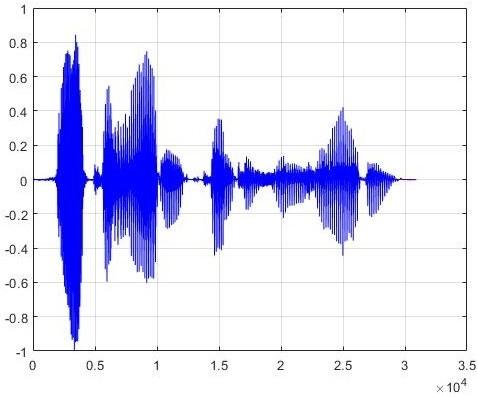
The pre-processing of the data is illustrated in Figure 2. The original form of the signal is shown in blue (Figure 2(a)), and the section highlighted in green is a chosen segment (Figure 2(b)). To extract the spectrograms, each bit of data was framed by division into subsections with a length of 128 through the Hamming window. The number of sampling points was determined as 128 to calculate the various Fourier transformations. For the images in the jpeg format created using this method, the DS1-1 dataset was used for the AHF emotions, and the DS1-2 dataset was employed for the BNS emotions.
(a) The original image of the signal
(b) Selected signal with centered-preprocessing
Figure 2. The process of signal pre-treatment for centered-preprocessing
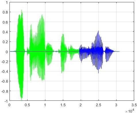
In the second method, general pre-processing, 19608 samples were taken from the beginning of the segment to establish the segments of a fixed length. Figure 3(a) shows the original form of the signal and Figure 3(b) represents the chosen segment highlighted in green. The spectrogram image of each chosen segment was taken. For the obtained images, the DS2-1 dataset was used for the AHF emotions and the DS2-2 dataset was employed for the BNS emotions.
(a) The original image of the signal
(b) Selected signal with general- preprocessing
Figure 3. The process of signal pre-treatment for general-preprocessing
Table 1. The appointed datasets
|
Dataset name |
Explanation |
|
DS1-1 |
The Spectrogram images for AHF with centered-preprocessing. |
|
DS1-2 |
The Spectrogram images for BNS with centered-preprocessing. |
|
DS2-1 |
The Spectrogram images for AHF with general-preprocessing. |
|
DS2-2 |
The Spectrogram images for BNS with general-preprocessing. |
|
DS3-1 |
MFCC features for AHF |
|
DS3-2 |
MFCC features for BNS |
In the last application of the present study, the features of MFCC were prepared as input for the DNN architecture to model the human ear [34]. When extracting the MFCC features employed in the application, the speech data were analyzed through the Hamming window with 256 ms and 0.5 overlaps. Log Fourier transform-based filter banks with 16 coefficients distributed on a Mel scale were extracted from each segment. Each MFCC coefficient was turned into a row vector by applying descriptive statistics (maximum, minimum, mean, standard deviation, skewness, kurtosis, and median), and the DS3-1 dataset was used for the AHF emotions and the DS3-2 dataset was employed for the BNS emotions.
In the present study, six different datasets were composed by extracting different features from the Emo-DB database, as illustrated in Table 1.
During the process of application, the triple groups, BNS and AHF, in the Emo-DB database were studied, which are the most frequently confused emotion groups, since the frequencies are very similar.
Evaluating the performance of the algorithm is an essential part of the study. To evaluate the success of the model, the matrices of the weighted accuracy (WA) and unweighted accuracy (UA) were employed.
The unweighted classification accuracy is the ratio of the number of correct predictions to the total number of samples Eq. (3). Where CP is number of correct predictions, and T is total number of samples.
$\mathrm{UA}=\frac{C P}{T}$ (3)
The weighted classification accuracy is the average of the ratios of the number of correct predictions in each class to the number of samples in same class Eq. (4). n is the number of classes. Where CPi is the number of correct predictions for i-th class and Ti is the total number of samples for i -th class.
$\mathrm{WA}=\frac{1}{\mathrm{n}} \sum_{i=1}^{n} \frac{C P^{i}}{T^{i}}$ (4)
3.1 CNN results
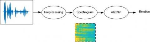
In the first application, the spectrogram images were given as the input for AlexNet. Figure 4 displays the process steps of the present study.
Figure 4. The scheme of classification of the speech signals through spectrogram images on AlexNet
With respect to the activation function of AlexNET, the function of ReLU was employed. The implemented parameters for the DS1-1 and DS1-2 datasets are displayed in Table 2; the convolutional filter size was accepted as 3 x 3, “the ReLU function” was employed for the activation function, and the dropout factor was accepted as 0.000075. The ADAM optimization algorithm was employed as the optimizer.
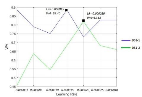
The initial learning rate started at a value of 0.000001, and its accuracy value was analyzed by increasing the initial value. As seen in Figure 5(a), the highest WA value for the DS1-1 dataset was a learning rate of 0.000015 (88.46%), whereas the highest WA value for the DS1-2 dataset was a learning rate of 0.00002 (81.82%).
Table 2. The network parameters for DS1-1, DS1-2, DS2-1, DS2-2 datasets
|
Parameter |
DS1-1 |
DS1-2 |
DS2-1 |
DS2-2 |
|
Convolution filter size |
3x3 |
3x3 |
3x3 |
3x3 |
|
Activation function |
ReLU |
ReLU |
ReLU |
ReLU |
|
Dropout factor |
0.000075 |
0.000075 |
0.0005 |
0.00015 |
|
Optimizer |
ADAM |
ADAM |
ADAM |
ADAM |
(a) The change of Learning rate-accuracy for DS1-1 and DS1-2
(b) The change of Learning rate-accuracy for DS2-1 and DS2-2
Figure 5. The change of accuracy for DS1-1, DS1-2, DS2-1 and DS2-2 in terms of learning rate
The network parameters for DS2-1 and DS2-2 are given in Table 2. In both the DS2-1 and DS2-2 datasets, the size of the convolutional filter was accepted as 3 x 3, the employed activation function was “the ReLU function,” and the dropout factor was 0.0005 for DS2-2 and 0.00015 for DS2-1.
Figure 5(b) shows the change in accuracy according to the learning rate of the DS2-1 dataset; the highest learning rate of 0.000025 was acquired with a WA of 80.77%. With respect to the DS2-2 dataset, a WA of 84.09% was obtained with a learning rate of 0.00001.
The WA and UA values are shown in Table 3; the WA was 88.46% for DS1-1 and 80.77% for DS2-1, while the UA values were 86.11% and 84.34%, respectively. Moreover, the WA for DS1-2 was 81.82% and for DS1-2 was 84.09%, and the UA for DS1-2 was 83.33% and for DS2-2 was 84.67%.
Table 3. Comparison of weighted accuracy (WA) and unweighted accuracy with AlexNet
|
Dataset Name |
WA |
UA |
|
DS1-1 |
88.46% |
86.11% |
|
DS1-2 |
81.81% |
83.33% |
|
DS2-1 |
80.77% |
84.34% |
|
DS2-2 |
84.09% |
84.67% |
3.2 DNN results
In the last part of the present study, 16 MFCC features were extracted from the speech data and descriptive statistics were performed (maximum, minimum, mean, standard deviation, skewness, kurtosis, and median), and the DS3-1 dataset was used for the AHF emotions and the DS3-2 dataset was employed for the BNS emotions (Figure 6). DS3-1 and DS3-2 were classified using DNN. The ReLU, Tanh, Sigmoid, Hard Sigmoid exponential and Softmax activation functions were employed. The number of neurons was tried between 16-512 by increasing 8 in all applications. The most successful structure was given. The ADAM and SGD algorithms were used as optimizers.
For the DS3-1 dataset, a network of four layers was established, consisting of 64 neurons each in the first, second, and third layers, and 3 neurons in the fourth layer. The activation functions employed in each layer are given in Table 4.
Table 4. The DNN parameters for DS3-1 and DS3
|
Parameters |
First layer |
Second layer |
Third layer |
Fourth layer |
|
|
DS3-1 |
Activation Function |
Tanh |
ReLU |
ReLU |
Softmax |
|
Neuron Numbers |
64 |
64 |
64 |
3 |
|
|
DS3-2 |
Activation Function |
Tanh |
Tanh |
ReLU |
Softmax |
|
Neuron Numbers |
128 |
128 |
64 |
3 |
|
Figure 6. Classification of MFCC attributes through DNN
Table 5. Comparison of weighted accuracy (WA) and unweighted accuracy with DNN
|
|
ADAM |
SGD |
||
|
WA |
UA |
WA |
UA |
|
|
DS3-1 |
76.67% |
75.56% |
75.00% |
72.42% |
|
DS3-2 |
82.35% |
83.19% |
78.43% |
79.44% |
The ADAM and SGD algorithms were employed as optimizers in the application; the results are given in Table 5. Employing the ADAM optimization algorithm gave a WA value of 82.35% for the DS3-2 dataset and 76.77% for the DS3-1 dataset. Using SGD, a WA value of 78.43% was obtained for the DS3-2 dataset and 75% for the DS3-1 dataset.
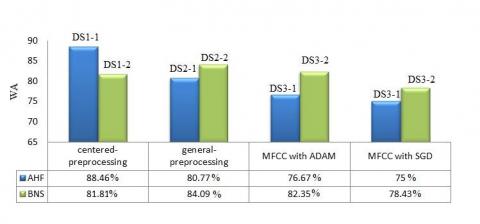
Figure 7 demonstrates that the highest achievement score was acquired with the DS1-1 dataset executed through the AlexNET architecture. In the AHF emotion group with the highest frequency, 76.77% was achieved with the DS3-1 dataset obtained from the manually extracted features, which was increased to 80.77% and subsequently to 88.46% through the use of spectrogram images. In the BNS emotion group, which consists of emotions with lower frequency levels, the best result was achieved with the DS2-2 dataset, where the spectrogram images were classified using AlexNET. A WA value of 82.35% was obtained in the DS3-2 dataset via DNN using MFCC features, and a WA value of 84.09% was obtained with the DS2-2 dataset. The results of the present study indicate that better results are achieved using spectrogram images as input as compared with applying DNN to manually extracted features.
Figure 7. The comparison of the WA results
In the literature, Demircan and Kahramanli [35] achieved a WA value of 78.08% for AHF, while in the present application; this value was increased to a maximum of 88.46% using the same emotion group. Moreover, BNS achieved a WA value of 80.00% [35], while this value was increased to 84.09% in the present study. They used Agent-Based Modelling and classified with ANN.
In the present study, two different approaches are presented related to the problem of recognizing emotions from speech. Firstly, the spectrogram images were classified using AlexNet, which is CNN architecture. Secondly, classification was conducted via DNN using the manually extracted MFCC features.
In the first application, the spectrogram images were acquired at a fixed length from the speech, and subsequently classified using AlexNET. In the second application, which employed the DNN architecture, manually extracted MFCC features that yield high results in this field were employed, after which they were transformed into features with fixed lengths using statistical functions, and classified using DNN. Separate trials were executed for ADAM and SGD optimization algorithms.
The best results were achieved with the DS1-1 dataset, where AlexNET was applied to the spectrogram images for the AHF emotion group, yielding a WA value of 88.46%. For the BNS emotion group, the best results were achieved with the DS2-2 dataset via AlexNET, achieving a WA value of 84.09%. It was found that application of the AlexNET architecture to spectrogram images was more discriminative than applying DNN to the manually extracted features.
One of the biggest problems with emotional databases is the amount of data; the scarcity of data is a disadvantage in deep learning. For that reason, we aim to apply different architectures of deep learning to databases that contain more data in future research.
S. Demircan thanks to Konya Technical University Scientific Research Projects for the support of this study. H. K. Örnek thanks to Selcuk University Scientific Research Projects for the support of this study the authors also thank TUBITAK for their support of this study.
[1] Gouizi, K., Reguig, F.B., Maaoui, C. (2011). Emotion recognition from physiological signals. Journal of Medical Engineering & Technology, 35(6-7): 300-7. http://dx.doi.org/10.3109/03091902.2011.601784
[2] Rahurkar, M., Hansen, J.H.L., Meyerhoff, J., Saviolakis, G., Koening, M. (2002). Frequency band analysis for stress detection using a Teager energy operator based feature. International Conference on Spoken Language Processing [ICSLP2002], Denver Colorado USA.
[3] Albert, M. (1970). A semantic space for nonverbal behavior. Journal of Consulting and Clinical Psychology, 35(2): 248-257. http://dx.doi.org/10.1037/h0030083
[4] Lee, E.T. (1994). Human emotion estimation through facial expressions. Kybernetes, 23(1): 39-46. http://dx.doi.org/10.1108/03684929410050568
[5] Rao, P., Choudhary, A., Kumar, V. (2019). 3D facial emotion recognition using deep learning technique. Review of Computer Engineering Studies, 6(3): 64-68. http://dx.doi.org/10.18280/rces.060303
[6] Wagner, J., Kim, J., Andre, E. (2005). From physiological signals to emotions: Implementing and comparing selected methods for feature extraction and classification. 2005 IEEE International Conference on Multimedia and Expo, pp. 940-943. http://dx.doi.org/10.1109/ICME.2005.1521579
[7] Ververidis, D., Kotropoulos, C. (2005). Emotional speech classification using gaussian mixture models and the sequential floating forward selection algorithm. 2005 IEEE International Conference on Multimedia and Expo, pp. 1500-1503. http://dx.doi.org/10.1109/ICME.2005.1521717
[8] Arias, J.P., Busso, C., Yoma, N.B. (2014). Shape-based modeling of the fundamental frequency contour for emotion detection in speech. Computer Speech & Language, 28: 278-294. http://dx.doi.org/10.1016/j.csl.2013.07.002
[9] Demircan, S., Kahramanli, H. (2017). Emotion recognition via agent-based modelling. 2017 25th Signal Processing and Communications Applications Conference – IEEE (SIU), pp. 1-4. http://dx.doi.org/10.1109/SIU.2017.7960513
[10] France, D.J., Shiavi, R.G., Silverman, S., Silverman, M., Wilkes, M. (2000). Acoustical properties of speech as indicators of depression and suicidal risk. IEEE Transactions on Biomedical Engineering, 47(7): 829-837. http://dx.doi.org/10.1109/10.846676
[11] Schuller, B., Rigoll, G., Lang, M. (2004). Speech emotion recognition combining acoustic features and linguistic information in a hybrid support vector machine - Belief Network architecture. 2004 IEEE International Conference on Acoustics, Speech, and Signal Processing, pp. 577-580. http://dx.doi.org/10.1109/ICASSP.2004.1326051
[12] Lefter, L., Rothkrantz, L.J.M., van Leeuwen, D.A., Wiggers, P. (2011). automatic stress detection in emergency (telephone) calls. International Journal of Intelligent Defence Support Systems, 4(2): 148-168. http://dx.doi.org/10.1504/IJIDSS.2011.039547
[13] Li, D., Yu, D. (2014). Deep learning: Methods and applications. Foundations and Trends® in Signal Processing, 7(3-4): 197-387. http://dx.doi.org/10.1561/2000000039
[14] Aizenberg, I., Aizenberg, N., Butakov, C., Farberov, E. (2000). Image recognition on the neural network based on multi-valued neurons. 15th International Conference on Pattern Recognition, Barcelona, Spain, 2: 989-992. http://dx.doi.org/10.1109/ICPR.2000.906241
[15] Hinton, G.E. (2007). Learning multiple layers of representation. Trends in Cognitive Sciences, 11: 428-34. http://dx.doi.org/10.1016/j.tics.2007.09.004
[16] Song, H.A., Lee, S.Y. (2013). Hierarchical Representation Using NMF. Neural Information Processing, Berlin, Heidelberg, pp. 466-473. http://dx.doi.org/10.1007/978-3-642-42054-2_58
[17] Zia, S., Yüksel, B., Yüret, D., Yemez, Y. (2017). RGB-D object recognition using deep convolutional neural networks. 2017 IEEE International Conference on Computer Vision Workshops (ICCVW), pp. 887-894. http://dx.doi.org/10.1109/ICCVW.2017.109
[18] Sulubacak, U., Eryigit, G. (2018). Implementing universal dependency, morphology, and multiword expression annotation standards for Turkish language processing. Turkish Journal of Electrical Engineering and Computer Sciences, 26: 1662-1672. https://doi.org/10.3906/elk-1706-81
[19] Yin, W.F., Yang, X.Z., Zhang, L., Li, L., Kitsuwan, N., Shinkuma, R., Oki, E. (2019). Self-adjustable domain adaptation in personalized ECG monitoring integrated with IR-UWB radar. Biomedical Signal Processing and Control, 47: 75-87. http://dx.doi.org/10.1016/j.bspc.2018.08.002
[20] Gorur, K., Bozkurt, M.R., Bascil, M.S. Temurtas, F. (2019). GKP signal processing using deep CNN and SVM for tongue-machine interface. Traitement du Signal, 36(4): 319-329. http://dx.doi.org/10.18280/ts.360404
[21] Hassan, Y.F. (2017) Deep learning architecture using rough sets and rough neural networks. Kybernetes, 46(4): 693-705. http://dx.doi.org/10.1108/K-09-2016-0228
[22] Sainath, T.N., Kingsbury, B., Sindhwani, V., Arisoy, E., Ramabhadran, B. (2013). Low-rank matrix factorization for deep neural network training with high-dimensional output targets. 2013 IEEE International Conference on Acoustics, Speech and Signal Processing, pp. 6655-6659. http://dx.doi.org/10.1109/ICASSP.2013.6638949
[23] Zhang, S.Q., Zhang, S.L., Huang, T.J., Gao, W. (2018). Speech emotion recognition using deep convolutional neural network and discriminant temporal pyramid matching. IEEE Transactions on Multimedia, 20(6): 1576-1590. http://dx.doi.org/10.1109/TMM.2017.2766843
[24] Ozseven, T. (2018). The acoustic cues of fear: Investigation of acoustic parameters of speech containing fear. Archives of Acoustics, 43(2): 245-251. https://doi.org/10.24425/122372
[25] Srivastava, N., Hinton, G., Krizhevsky, A., Sutskever, I., Salakhutdinov, R. (2014). Dropout: A simple way to prevent neural networks from overfitting. Journal of Machine Learning Research, 15(1): 1929-1958.
[26] Bengio, Y. (2009). Learning deep architectures for AI. Foundations and Trends in Machine Learning, 2(1): 1-127. http://dx.doi.org/10.1561/2200000006
[27] Fayek, H.M., Lech, M., Cavedon, L. (2017). Evaluating deep learning architectures for speech emotion recognition. Neural Networks, 92: 60-68. http://dx.doi.org/10.1016/j.neunet.2017.02.013
[28] Kingma, D.P., Ba, J.L. (2014). Adam: A method for stochastic optimization. International Conference on Learning Representations, p. 15.
[29] Şeker, A., Diri, B., Balık, H.H. (2017). Derin Öğrenme Yöntemleri ve Uygulamaları Hakkında Bir İnceleme. Gazi Mühendislik Bilimleri Dergisi, 3: 47-64.
[30] LeCun, Y., Bengio, Y., Hinton, G. (2015). Deep learning. Nature, 521: 436-444. http://dx.doi.org/10.1038/nature14539
[31] Krizhevsky, A., Sutskever, I., Hinton, G. (2012). ImageNet Classification with deep Convoutional Neural Network. NIPS'2012.
[32] Burkhardt, F., Paeschke, A., Rolfes, M.A., Sendlmeier W.F., Weiss, B. (2005). A database of German emotional speech. INTERSPEECH.
[33] Ma, X., Wu, Z., Jia, J., Xu, M., Meng, H., Cai, L.(2018). Emotion recognition from variable-length speech segments using deep learning on spectrograms. Proc. Interspeech 2018, pp. 3683-3687. http://dx.doi.org/10.21437/Interspeech.2018-2228
[34] Becchetti, C., Ricotti, L.P. (1999). Speech Recognition: Theory and C++ Implementation. Wiley.
[35] Demircan, S., Kahramanli, H. (2018). Application of ABM to spectral features for emotion recognition. Mehran University Research Journal of Engineering and Technology, 37: 453-462. http://dx.doi.org/10.22581/muet1982.1804.01