Omer Akgun
© 2020 IIETA. This article is published by IIETA and is licensed under the CC BY 4.0 license (http://creativecommons.org/licenses/by/4.0/).
OPEN ACCESS
In this study, the internal or superficial cracks that may occur during the production of ceramic plates were determined using the impact noise method. In the industry, ceramic materials are frequently used in areas such as kitchenware and construction. Many different methods are used in the quality control processes of ceramic materials. In this study, the sound produced by the impact applied to the ceramic material was analyzed. As a result of the analysis, the material was found to be undamaged or damaged. This method is called the Impulse Noise method. In this study, damaged and undamaged ceramic plates with different cracks were selected and impact plates were applied to the plates by impact pendulum. The ceramic plates used in the application have the same characteristics and dimensions produced by the same company of the same type. The noise generated as a result of the impact applied to a determined point on the tested materials was examined by Wigner-Ville method which is one of the time-frequency analysis methods. In addition, bispectrum and trispectrum analyzes, which are high-order spectral analysis (HOSA) methods, were used. Statistically, signal analysis with running minimum and maximum, mean value and peak to RMS examinations were also added. The applied methods give good results in differentiating between undamaged and damaged ceramic plates.
ceramic materials, crack analysis, impulse noise method, Wigner Ville distribution, bispectrum, trispectrum, mean value, Peak to RMS
Inorganic compounds made by metals or semi-metals with non-metallic elements are called ceramics. A wide range of inorganic materials including materials such as clay, sand and feldspar. Ceramics are very fragile. The brittle fracture occurs with the formation and propagation of cracks. Crack growth may be transgranular or intergranular. It is also known that ceramic is a very good sound reflector.
Ceramic is one of the oldest tools used by people. For centuries, the superior qualities of ceramics have been utilized, especially in the construction of pots and pans. The abundance of raw materials, easy processing, simple manufacturing, relatively low cost, ease of use etc. with reasons; hardness, heat resistance, such as the positive effects of the use increases [1-4].
Today, the ceramic and porcelain industry are mainly active in the kitchen and construction sectors. Many of the damages that occur before or after the marketing of ceramic materials to end-users are economically costly. In this sense, cracks and deformations that may occur in the material during or after stacking, which can be seen or not visible, are among the most important problems that manufacturers must solve. These defects cause economic losses and loss of time. For this reason, it is of great importance in the ceramic-porcelain industry that defects in damaged materials are solved by pre-sales final checks by very fast and simple methods [5, 6].
Different testing methods are used in the ceramic industry after production. It is known that these methods are made with large test equipment in the factory environment. X-Ray is the most effective method for determining damage, especially in ceramic materials. This method provides important and effective analyzes of ceramic and porcelain materials in terms of their chemical structure and determination of post-production damage in practice [7, 8]. However, these methods are much more effective for raw material analysis and offer significant contributions to the development of the chemical process. It is used in the diagnosis of cracks in ceramic and porcelain materials and in different methods in practice [9].
In this study; impulse noise method, which can be counted among ultrasonic methods, has been used [10, 11]. The mechanical system in the experimental study was established in order to hit the same impact on ceramic materials (pendulum). With the experimental system, the same intensity impact can be applied to ceramic materials. The pendulum was used for an equal blow. The sound emitted from the material by the impact applied to the ceramic material is quaint with the microphone. It is aimed to analyze sounds by recording sounds applied to ceramic materials with strong and different cracks in a similar way [12-14].
One of the spectral analysis methods, Wigner-Ville is a time-frequency method. It was derived by Wigner in the field of quantum mechanics and later expanded by Ville for signal processing [15]. Various methods can be used to design such a time-frequency representation, the simplest approach being to divide the signal into short time segments and determine the spectrum of each segment by Fourier transform. The result of this process is the commonly used short-time fourier transform (STFT) [16-18]. By analyzing the frequency content of the signal as the time window moves, a time-frequency distribution called spectrogram (square of the size of the STFT) is generated. It has the advantage of being positive, easy to interpret, but also has the disadvantage of being irreversible. This means that once the spectrogram of a signal is calculated, the original signal cannot be obtained from the spectrogram again [18]. The theory of WV, which will be briefly discussed in the following sections of the study, gives very satisfactory results in this sense.
In signal processing methods utilizing quadratic statistics and / or power spectrum, phase relationships between frequency components are not considered; therefore, these methods are blind to phase information. In addition, second-order statistics and power spectra are not sufficient to accurately define non-gaussian processes [19, 20]. Second-order statistics such as autocorrelation and power spectral density provide important information in the analysis of gauss, stationary and linear processes. The autocorrelation function is not sufficient for non-Gaussian processes. In this study, more information can be obtained from these processes by higher-order spectral analysis (HOSA) methods such as bispectrum and trispectrum [19, 21]. The study was supported statistically by providing graphs with running minimum and maksimum, mean value and peak to RMS graphs of the signals.
2.1 Wigner Ville distribution
Another well-known disadvantage of STFT is the resolution limit imposed by the window function. A shorter time window results in better resolution but results in poorer frequency resolution, and vice versa. One of the most important methods to be used here is the analysis known as quadratic or bilinear time-frequency distribution. The main member of this class is the Wigner-Ville distribution (WVD). All other time-frequency conversions can be written as a smoothed version of WVD [17, 22-24]. WVD provides many of the features required for some specific applications of non-stationary signal analysis.
Perhaps the most significant feature of the Wigner distribution is the effect it has for the gaussian windowed linear chirp signal.
For the $x(t)=e^{-c t^{2}} e^{j\left(a_{0}+a_{1} t+a_{2} t^{2}\right)}$ signal, the wigner distribution condenses energy along with the instantaneous frequency of the signal. Wigner Distribution of the signal is given as $W_{x}(t, w)=e^{-\left(w-a_{1} t-2 a_{2} t^{2}\right) / 2 c} e^{-2 c t^{2}}$ [15].
In Eq. (1), the WVD expression of an x(t) time signal is given [25].
$W V D(t, w)=\int_{-\infty}^{\infty} x\left(t+\frac{\tau}{2}\right) x^{*}\left(t-\frac{\tau}{2}\right) e^{-j w t} d \tau$ (1)
where, x(t) is the time series of the signal, x*(t) is the complex conjugate of the signal, t instantaneous time, w instantaneous frequency, τ time delay. The most important problem of Wigner-Ville distribution is cross terms. The cross-terms formed between the two strong frequency components can be eliminated using the smoothed Wigner-Ville distribution.
$\begin{array}{l}
\operatorname{SPW}(t, w)= \\
\int_{-\infty}^{\infty} \int_{-\infty}^{\infty} x\left(t+\frac{\tau}{2}\right) x^{*}\left(t-\frac{\tau}{2}\right) g(v) h(\tau) e^{-j w t} d v d \tau
\end{array}$ (2)
where, v is the balancing frequency, g(v) is the softened window in the frequency space and h(τ) is the softened window in the time-space [26, 27].
2.2 Bispectrum
The application of higher-order spectral analysis in the analysis of signals which are not in the stationary, linear and gauss forms is more advantageous than power spectrum analysis in terms of revealing phase-related information as well as spectral information within the signal. Bispectrum analysis, which is one of the higher-order analysis methods, is a successful method for detecting quadratic phase coupling (QPC) between the components of the signal [28]. Higher-order statistics are provided with higher-order moments, such as (Eq. (3), (4)). The nonlinear combinations of these higher-order moments are known as cumulants (Eq. (5)-(7)) [29].
$m_{X}^{3}(i, j)=E\{X(n) . X(n+i) . X(n+j)\}$ (3)
$m_{X}^{4}(i, j, k)=E\{X(n) . X(n+i) . X(n+j) . X(n+k)\}$ (4)
Stack equations for the zero-mean process;
$c^{2}(i)=m(i)$ (5)
$c^{3}(i, j)=m(i, j)$ (6)
$\begin{array}{l}
c^{4}(i, j, k)=m^{4}(i, j, k)-m^{2}(i) m^{2}(j, k) \\
-m^{2}(j) m^{2}(i, k)-m^{2}(k) m^{2}(i, j)
\end{array}$ (7)
In addition to suppressing gaussian probability distributed activity, the bispectrum reveals data from the nonlinear process. Bispectral analysis; it is used to detect low-level, but important, diagnostic signals masked by background data [19, 30].
The power spectrum of random signals is defined by the discrete fourier transform (DFT), (Eq. (8)).
$P_{2}^{x}(f)=D F T \quad\left(C_{2}^{x}(m) \cdot e^{-j 2 \pi m f}\right.$ (8)
The 3rd order stack spectrum is called bispectrum.
$B^{x}\left(f_{1}, f_{2}\right)=\sum_{m=-\infty}^{\infty} \sum_{n=-\infty}^{\infty} C_{3}^{x}(m, n) \cdot e^{-j 2 \pi\left(m f_{1}+n f_{2}\right)}$ (9)
or (if the signal reel is a stationary random process)
$B\left(w_{1}, w_{2}\right)=X\left(w_{1}\right) \cdot X\left(w_{2}\right) \cdot X^{*}\left(w_{1}+w_{2}\right)$ (10)
2.3 Trispectrum
The power spectrum of a continuous x(t) signal is expressed by the following Eq. (11), where the Fourier transform of the signal is X(f).
$S(f)=E\left[X(f) X^{*}(f)\right]$ (11)
In Eq. (11), * indicates conjugation and E[ ] is the expected value.
Bispectrum B(f1, f2) and trispectrum T(f1, f2, f3). They can be expressed as Eqns. (12) and (13) respectively.
$B\left(f_{1}, f_{2}\right)=E\left[X\left(f_{1}\right) X\left(f_{2}\right) X^{*}\left(f_{1}+f_{2}\right)\right]$ (12)
$\begin{array}{l}
T\left(f_{1}, f_{2}, f_{3}\right)= \\
E\left[X\left(f_{1}\right) X\left(f_{2}\right) X\left(f_{3}\right) X^{*}\left(f_{1}+f_{2}+f_{3}\right)\right]
\end{array}$ (13)
The above frequency expression of the bispectrum contains three frequency interactions (Eq. (14)).
$B\left(f_{1}, f_{2}, f_{3}\right)=E\left[X\left(f_{1}\right) X\left(f_{2}\right) X\left(f_{3}\right)\right]$ (14)
where, $f_{3}=-f_{1}-f_{2}$
Similarly, it can be shown in the trispectrum using four frequency notations (Eq. (15)) [31, 32].
$T\left(f_{1}, f_{2}, f_{3}, f_{4}\right)=E\left[X\left(f_{1}\right) X\left(f_{2}\right) X\left(f_{3}\right) X\left(f_{4}\right)\right]$ (15)
where, $f_{4}=-f_{1}-f_{2}-f_{3}$
In the study, firstly ARMA parameters of 4th grade cumulants were obtained. The auto-regressive moving-average (ARMA) process is a useful model for time series analysis (Eq. (16)) [33].
$x(n)=-\sum_{k=1}^{p} a(k) x(n-k)+\sum_{k=0}^{q} b(k) u(n-k)$ (16)
Then the trispectrum was calculated by taking f3=0.5 by using auto-regressive (AR) parameters and moving-average (MA) parameters.
2.4 Mean value and peak to RMS
The mean value of a function can be written as in Eq. (17) below:
$E[f]=\sum_{x} p(x) f(x)$ (17)
where, E in Eq. (17) is the mean value. In fact, the mean value calculation is simply a weighted average. In other words, for any x value, the result of this value in function f is multiplied by the probability of occurrence of this x event [34].
The RMS of a signal is calculated from the peak amplitude, the peak to peak amplitude value, or the average value of the signal. The RMS value for each is calculated based on the following statements.
$V_{r m s}=\frac{1}{\sqrt{2}} * V_{P}=0.707 * V_{P}$ (18)
$V_{r m s}=\frac{1}{2 \sqrt{2}} * V_{P-P}=0.353 * V_{P-P}$ (19)
$V_{r m s}=\frac{\pi}{2 \sqrt{2}} * V_{a v g}=1.111 * V_{a v g}$ (20)
where, Vavg is the level of a waveform defined by the condition that the area enclosed by the curve above this level is exactly equal to the area enclosed by the curve below this level (Eq. (20)) [35]. Vrms is the root-mean-square or effective value of a waveform (Eq. (18)-(20)). VP is the maximum instantaneous value of a function measured from the Zero level (Eq. (18)). VP-P, Full amplitude of waveform between positive and negative peaks; that is, the sum of the positive and negative peaks (Eq. (19)). Vavg, the level of a waveform. This equation is equal to this level (Eq. (20)) [35].
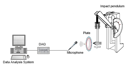
Testing set, developed by Akinci [12], was used in this study and the data were obtained from this testing set. Pendulum was used in order to produce impact in experimental measurement and data collection systems [12, 36]. An impact of determined size was inflicted to the ceramic plate through a plastic hammer connected to the end of impact pendulum and sound, emerged from the plate as a result of the impact, was recorded by the microphone and data collection system [12, 37, 38].
Figure 1. Data acquisition and measurement systems [12]
The POE 2000 type Impact Pendulum was used in experimental data collection system. Impacts in the same severity were applied to the ceramic plates of same type and model through pendulum and the sound data, which emerged as a result of impact, had been recorded. The output audio signal of the amplifier is transmitted to the computer at a sampling rate of 0.00001 seconds via Advantech 1716 L Multifunction PCI card and data processing is performed by using Matlab © (Figure 1) [12, 38].
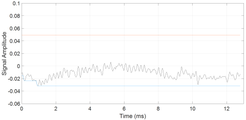
When undamaged plate data is examined, it starts from 0 and 0.05 max. amplitude up to (2.5 ms), a period of this amplitude of the mold after the running maximum close to the end by making fluctuations. The running minimum started with an amplitude of -0.01, but the signal never came down to this level again. The undamaged plate analysis graph draws attention with its high amplitude character (Figure 2(a)).
The first damaged plate data never reached the running max. of 0.05 amplitude. After progressing with peaks of approximately 0.04 amplitude up to 2.5 ms, it quickly dropped to a running min. of -0.01 amplitude up to 6 ms. The running minimum amplitude has fallen a little further, ending the signal with peaks close to this running (Figure 2(b)).
The second damaged signal started with a running minimum of -0.01 amplitude, then reduced to a running minimum level of -0.3 amplitude, and the rest of the marker ended in progress near the running minimum level far from the running maximum level of 0.05 amplitude (Figure 2(c)).
Damaged plate data are noted for their low amplitude characteristics, close to the running minimum level.
a)
b)
c)
Figure 2. Signal with running Minimum and Maximum (a) Undamaged (b) and (c) Damaged ceramic plates
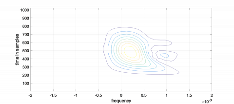
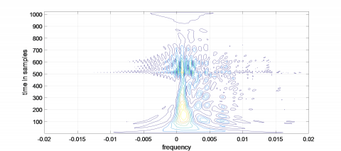
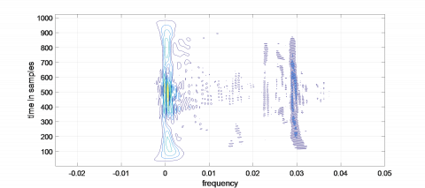
Undamaged ceramic data The WV map contains a large formation of intertwined rings (high to low peaks) over a wide frequency range and a small formation of two low amplitude peaks next to it. The undamaged data is remarkable with its simple structure (Figure 3(a)).
In the WV map of the first damaged signal, the main region extending over a long period of time in the narrow frequency range and small multi-particle formations spread around the region were observed (Figure 3(b)).
In the second damaged signal WV map, there is an all-time (more uniform and thinner) structure in the narrow frequency range and around the structure, although not as many as the first, fragmented regions. In addition, around the frequency of 0.03 Hz, there was a bar area consisting of dense small peaks extending along the time axis, and there were fragmented thin formations around it (Figure 3(c)).
Damaged data is observed to have multi-part structures.
a)
b)
c)
Figure 3. (a) Undamaged (b) and (c) WV maps of the signals of damaged ceramic plates
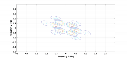
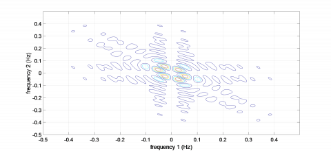
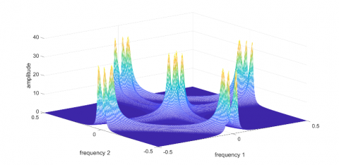
On the equiphase surface of the undamaged plate there is a first ring with high peaks, and a second ring with low amplitude peaks around it (Figure 4(a)).
The first damaged data includes two rings of small amplitude peaks in addition to the structures in the undamaged data (Figure 4(b)). In the second damaged signal, the main formation took place at lower frequencies. Around it is low amplitude peaks in more numerous and distorted formations than in the first damaged data (Figure 4(c)).
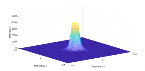
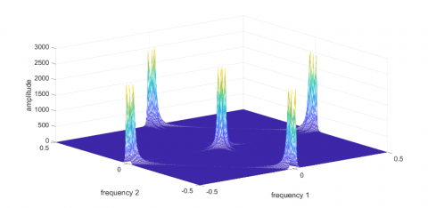
The 3-dimensional trispectrum map of the signal of the undamaged data consisted of a high amplitude peak at its origin, with f3=0.5 (Figure 5(a)).
The trispectrum of the first damaged signal consisted of five peaks with a lower amplitude than that of the intact data, one at the centre and one at each side of the surface, again with f3=0.5 (Figure 5(b)). The three-dimensional trispectrum of the second damaged data, on the other hand, was composed of 5 main peaks, similar to that of the other damaged sign, when f3=0.5. Here, the peak amplitudes are very small compared to others. In addition, extensions that connect each hill with each other are also noteworthy (Figure 5(c)). Damaged signals with undamaged plate signal, single peak simple structure and high amplitude have 5 peak and low amplitude shapes.
a)
b)
c)
Figure 4. a) Undamaged b) and c) Bispectrum maps of data on damaged ceramic plates
a)
b)
c)
Figure 5. (a) Undamaged (b) and (c) Trispectrum maps of data on damaged ceramic plates
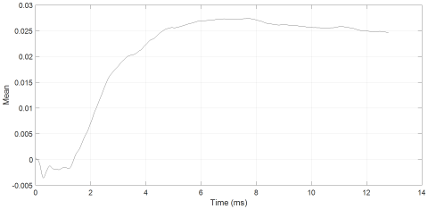
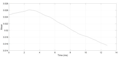
In the mean value graph of undamaged plate signals, a curve increased to about 0.025 amplitude in about 5 ms, followed by a graph that retains the same amplitude to the end of time (Figure 6(a)).
In the first damaged graph, the curve (0.026 amplitude) showing a small increase up to 3ms, followed by a graph with a decrease in amplitude up to about zero. (Figure 6(b)). On the other damaged graph, a curve with a continuous decrease in amplitude was detected from the beginning to the end of time (Figure 6(c)).
a)
b)
c)
Figure 6. (a) Undamaged (b) and (c) Mean value graphs of data analysis of damaged ceramic plates
In the mean value analysis, the undamaged signal has a rising amplitude graph and the damaged signals have a falling amplitude graph.
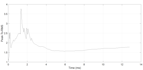
In the undamaged ceramic plate signal peak to RMS analysis, a peak of up to 5 ms is noted. The peak of this hill is 3.8 amplitude around 1ms. After this peak went down to 1.5 amplitude, the graph continued at the same level until the end of time (Figure 7(a)).
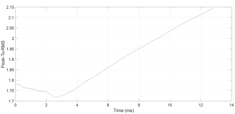
The first damaged signal forms a graph with a small descent of up to 3 ms and then up to 2.15 amplitude by the end of time (Figure 7(b)). The second damaged signal produced a graph starting at 2.15 amplitude and rising up to 2.4 (Figure 7(c)). In Peak to RMS, robust data is characterized by an initial peak and a curve that retains its amplitude, while damaged data is characterized by rising graphs.
a)
b)
c)
Figure 7. (a) Undamaged (b) and (c) Peak to RMS graphs of data on damaged ceramic plates
In this study, signal analysis of internal or superficial cracks in ceramic plates was performed using the impact noise method. In particular, ceramic materials produced as kitchen utensils show the defects such as deformation under the glazes and cracks, in the form of deepening or breaking of the cracks by putting hot or cold foods inside. This is shown as unwanted errors for manufacturers. In the quality control of ceramic materials, tests performed by X-Ray and experts are frequently used in practice. In this study, an approach has been obtained on whether or not the ceramic plates are deformed by the impact noise obtained after the application of impact on the ceramic plates. This method can also be shown as a new method in practice. In this study, time-amplitude analysis with running minimum and maximum were applied to the signals obtained by the impact noise method using plates produced from the same material. In this analysis, undamaged signal was noted for their high amplitude and damaged signals for their low amplitude characteristics. Then, the cracks on the material were examined on the maps obtained using spectral analysis methods. First, Wigner spectra are discussed. The signal of the undamaged plate has a simple formation, whereas the damaged data is generated by multipartications. In bispectrum analysis, the undamaged plate appears as two-ring equiphase surfaces in it signals, while the damaged signals have multi-ring and distorted equiphase surfaces. In the trispectrum analysis, another high-order spectral analysis method, the undamaged signal appeared as a single high-amplitude peak, while the damaged signals were noted for their formation with much lower amplitude and a total of five peaks distributed over the surface. The data were also subjected to simple statistical analysis (time amplitude analysis with running minumum maximum, which is at the beginning of the analyzes, is actually a simple statistical analysis). Undamaged signal was observed with rising mean value graph and damaged signals were observed with descending mean value graph values. In the Peak to RMS examination, the undamaged signal was identified by a peak-peak and a curve that retains its amplitude, while the damaged signals were identified by their ascending graph. The applied methods have been very good at distinguishing between undamaged and damaged ceramic plates.
[1] Calıskan, F. (2016). Ceramic materials course. Sakarya University, Faculty of Technology, Department of Metallurgical and Materials Engineering.
[2] Gökbel, F. (2019). The relationship between ceramic material and sound. Dumlupınar University, Journal of Social Sciences, 51-66. http://dergipark.gov.tr/download/article-file/668587
[3] Kalemtas, A. (2019). Ceramic materials. Metallurgical and Materials Engineering Department, Muğla Sıtkı Kocman University.
[4] Li, B. (2014). Numerical and experimental analysis of crack propagation behaviour for ceramic materials. Materials Research Innovations, 18(6): 418-429. https://doi.org/10.1179/1433075X13Y.0000000169
[5] Perez, J. (2016). Ceramic Materials: Synthesis, Performance and Applications. Nova Science Publishers New York, USA.
[6] Ralph, B., Xiao, P. (2009). Advances in Ceramic Materials. Trans Tech Publications Ltd., Zurich, Switzerland.
[7] Skacel, J., Otahal, A., Szendiuch, I., Hejatkova, E. (2018). X-ray inspection of ceramic structures. 2018 41st International Spring Seminar on Electronics Technology (ISSE), Zlatibor, Serbia, pp. 1-4. https://doi.org/10.1109/ISSE.2018.8443652
[8] Blanton, T. (2017). Ceramic materials characterization using X-ray diffraction. Ceramic Industry, 167(5): 24-28.
[9] Lan, S., Zheng, X. (2015). Research on computer aided defect recognition of ceramic crack. Seventh International Conference on Measuring Technology and Mechatronics Automation, Nanchang, China, pp. 852-855. https://doi.org/10.1109/ICMTMA.2015.210
[10] Goncharov, V., Novic, A. (2018). Study of ceramic materials ultrasonic dispersion. Smart Nanocomposites, 8(2): 319-321.
[11] Baraheni, M., Amini, S. (2019). Predicting subsurface damage in silicon nitride ceramics subjected to rotary ultrasonic assisted face grinding. Ceramics International, 45(8): 10086-10096. https://doi.org/10.1016/j.ceramint.2019.02.055
[12] Akinci, T.C. (2011). The defect detection in ceramicmaterials based on time-frequency analysis by using the method of impulse noise. Archives of Acoustics, 36(1): 1-9. https://doi.org/10.2478/v10168-011-0007-y
[13] Akinci, T.C., Nogay, H.S., Yilmaz, O. (2012). Application of artificial neural networks for defect detection in ceramic materials. Archieves of Acoustics 37(3): 279-286. https://doi.org/10.2478/v10168-012-0036-1
[14] Akinci, T.C., Seker, S., Gurbuz, R., Guseinoviene, E. (2013). Spectral and statistical analysis for ceramic plate specimens subjected to impact. Solid State Phenomena, 199: 621-626. https://doi.org/10.4028/www.scientific.net/SSP.199.621
[15] Cekic, Y. (2004). Time-Frequency Analysis for Non-Stationary Signals. European Association for Signal Processing.
[16] Bzikha, I., Guiffaut, C., Reineix, A. (2019). Time-Frequency analysis for wiring soft faults detection. 2019 International Symposium on Electromagnetic Compatibility - EMC EUROPE, Barcelona, Spain, pp. 481-485. https://doi.org/10.1109/EMCEurope.2019.8871449
[17] Thomas, M., Jacob, R., Lethakumary, B. (2012). Comparison of WVD based time-frequency distributions. International Conference on Power, Signals, Controls and Computation (EPSCICON), Kerala, India. https://doi.org/10.1109/EPSCICON.2012.6175242
[18] Rybak, G., Chaniecki, Z., Grudzien, K., Romanowski, A., Sankowski, D. (2018). Performance analysis of short-time fourier transform algorithm with selected optimization methods. International Interdisciplinary PhD Workshop (IIPhDW), Swinoujście, Poland, pp. 371-376. https://doi.org/10.1109/IIPHDW.2018.8388393
[19] Akgun, O. (2011). Analysıs of Heart Sound Sıgnals in Mıtral Valve Dıseases. Doctoral thesis, Marmara University, Istanbul, Turkey.
[20] Başar, R., Artan, U., Akan, A. (2003). Higher order evolutionary spectral analysis. IEEE ICASSP 6, Hong Kong, China, pp. 633-636. https://doi.org/10.1109/ICASSP.2003.1201761
[21] Chua, K.C., Chandran V., Rajendra Acharya, U., Lim, C.M. (2009). Analysis of epileptic EEG signals using higher order spectra. Journal of Medical Engineering and Technology, 33(1): 42-50. https://doi.org/10.1080/03091900701559408
[22] Lu, F.P., Wang, H.X., Liu, X., Liu, C.H., Kang, J.F., Miao, X.J. (2016). Time-frequency characteristics of PSWF with Wigner-Ville Distributions. 2016 IEEE International Conference on Signal and Image Processing (ICSIP), Beijing, China, pp. 568-572. https://doi.org/10.1109/SIPROCESS.2016.7888326
[23] Boualem, B. (2016). Signal Analysis Using Wigner-Ville Spectrum. Elsevier, Amsterdam, Netherlands.
[24] Akdeniz, F., Kayikcioglu, I., Kaya, I., Kayikcioglu, T. (2016). Using Wigner-Ville distribution in ECG arrhythmia detection for telemedicine applications. 39th International Conference on Telecommunications and Signal Processing (TSP), Vienna, Austria, pp. 409-412. https://doi.org/10.1109/TSP.2016.7760908
[25] Pachori, R.B., Sircar, P. (2008). Time-frequency analysis using time-order representation and Wigner distribution. TENCON 2008 - 2008 IEEE Region 10 Conference, Hyderabad, India. https://doi.org/10.1109/TENCON.2008.4766782
[26] Kayıkcıoglu, I., Ulutas, G., Akdeniz, F., Kayıkcıoglu, T. (2018). Early detection of ST change based on Wigner-Ville distrubition. Süleyman Demirel University Journal of Natural and Applied Sciences, 22(2): 746-753. https://doi.org/10.19113/sdufbed.40216
[27] Kalra, M., Kumar, S., Das, B. (2019). Target detection using smooth pseudo Wigner-Ville distribution. 2018 IEEE Recent Advances in Intelligent Computational Systems (RAICS), Thiruvananthapuram, India, pp. 6-10. https://doi.org/10.1109/RAICS.2018.8635078
[28] Sezgin, N. (2016). Classification of epileptic EEG signals by extreme learning machines. Dicle University Faculty of Engineering, Journal of Engineering, 7(3): 481-490.
[29] Wang, A., Li, R. (2019). Research on digital signal recognition based on higher order cumulants. International Conference on Intelligent Transportation, Big Data & Smart City (ICITBS), Changsha, China, pp. 586-588. https://doi.org/10.1109/ICITBS.2019.00146
[30] Yang, D.M. (2017). The envelop-based bispectral analysis for motor bearing defect detection. 2017 International Conference on Applied System Innovation (ICASI), Sapporo, Japan, pp. 1646-1649. https://doi.org/10.1109/ICASI.2017.7988250
[31] Collis, W.B., White, P.R., Hammond, J.K. (1998). Higher-order spectra: The bispectrum and trispectrum. Mechanical Systems and Signal Processing, 12(3): 375-394). https://doi.org/10.1006/mssp.1997.0145
[32] Bhalke, D.G., Rao, C.B.R., Bormane, D.S (2014). Musical instrument classification using higher order spectra. International Conference on Signal Processing and Integrated Networks (SPIN), Noida, India, pp. 40-45. https://doi.org/10.1109/SPIN.2014.6776918
[33] Swami, A., Mendel, J.M., Nikias, C.L. (1998). Higher-Order Spectral Analysis Toolbox, The MathWorks.
[34] Evrenseker, S. Expected Value, http://bilgisayarkavramlari.sadievrenseker.com/2013/01/23/expected-value-beklenen deger/, accessed on 5 January 2020.
[35] RMS Voltage Calculator, https://www.allaboutcircuits.com/tools/rms-voltage-calculator/, accessed on 5 January 2020.
[36] Suzuki, M., Ogawa, K., Shoji, T. (1985). Quantitative NDE of surface cracks in ceramic simple pendulum approximation. Am. J. Phys, 53(1): 73-76.
[37] Suzuki, M., Ogawa, K., Shoji, T. (2006). Quantitative NDE of surface cracks in ceramic materials by means of a high-frequency electromagnetic wave. Materials Transactions, 47(6): 1605-1610. https://doi.org/10.2320/matertrans.47.1605
[38] Akinci, T.C., Yilmaz, O., Kaynas, T., Ozgiray, M., Seker, S. (2011). Defect detection for ceramic materials bey continuous wavelet analysis. Mechanika, Prooceedings of the 16th International Conference, Kaunas, Lithuana, pp. 9-14.