Jianhua Zhang* | Qiang Zhu | Lin Song
© 2019 IIETA. This article is published by IIETA and is licensed under the CC BY 4.0 license (http://creativecommons.org/licenses/by/4.0/).
OPEN ACCESS
This paper attempts to construct a suitable wavelet for image denoising based on wavelet thresholding algorithm. First, the author discussed how image thresholding is affected by the wavelet orthogonality and bi-orthogonality, the features of vanishing moments and the odd or even symmetry of the decomposition end filter. The discussion shows that the most desirable wavelet for image denoising is the biorthogonal wavelet, in which the decomposition end filter has zero point even symmetry, the low-pass decomposition enjoys a wide support interval, and the high-pass decomposition filter has a short support and attenuates fast. On this basis, three zero point even symmetric biorthogonal wavelets with different vanishing moment features were developed through the parametric construction of fixed-length tightly-supported (FLTS) biorthogonal wavelet, and a self-adaptive hierarchical thresholding algorithm was designed. The simulation results show that the developed wavelets have excellent denoising ability and enhance the images with rich details. Coupled with the self-adaptive hierarchical thresholding algorithm, these wavelets can effectively improve the image quality.
wavelet analysis, image denoising, parametric construction of biorthogonal wavelet, self-adaptive hierarchal thresholding
Fourier transform is the most popular denoising method in engineering. But the Fourier transform has a severe limitation in the positioning of the time and frequency domains. This limitation can be overcome by wavelet analysis, a multi-resolution (multi-scale) representation method for signals or images. The wavelet analysis can simultaneously provide the signal or image information in the time (space) and frequency domains [1-3]. Whereas the Fourier transform relies on a single triangular basis function, the wavelet analysis can select wavelet functions flexibly according to signal features and denoising requirements, and choose from various forms of wavelet transforms, such as multiwavelet or wavelet packet. In the wavelet transform domain, noise smoothing is selective in both space and frequency, which overcomes the limitation of Fourier transform.
Image denoising is not a new topic. In the past, however, only linear filtering methods have been adopted to denoise images. The wavelet theory and its application in 2D images provide a better solution to image denoising, and promote the progress in this field. Based on the wavelet theory, the noisy signals are subject to wavelet transform. The filtered signals differ greatly from the noises in wavelet coefficient on different scales. Then, the wavelet coefficients of signals and noises are processed by different sets of rules, aiming to reduce or eliminate the coefficients of noises. Meanwhile, the wavelet coefficients of the original signals are retained as much as possible. Finally, the original signals are reconstructed through inverse wavelet transform [4].
There are various denoising methods based on wavelet analysis. The most popular one is wavelet thresholding [5]. This method enjoys many advantages. For example, the edge information of the images can be retained well through multi-resolution analysis; the algorithm runs fast due to the relatively small computing load; the method supports multiple scales and various directions in local areas of time and frequency domains. The wavelet thresholding can pinpoint signals accurately and suppress noises, creating high-quality processed images. There are two types of wavelet thresholding, namely, soft thresholding and hard thresholding. Nonetheless, there are some defects with the two approaches. If an image is denoised with a soft threshold function, the edges of the processed image might be blurry; if the image is denoised with a hard threshold function, pseudo Gibbs phenomenon and the ringing artefact tend to occur [6], leading to visual distortion.
Other commonly used wavelet denoising algorithms also have obvious limitations. For instance, the wavelet transform modulus maxima (WTMM) method cannot achieve satisfactory denoising effect, because its calculation accuracy is affected by various factors [7, 8]. In correlation-based wavelet denoising, the noises can be suppressed effectively through multi-layer decomposition, but few details are available through the decomposition. What is worse, the wavelet coefficients will have small offsets on various scales, making the inter-layer correlation coefficients inaccurate and distorting the reconstructed signals.
To solve the problems, this paper puts forward a novel image thresholding method based on wavelet. First, the author explored how image thresholding is affected by the wavelet orthogonality and bi-orthogonality, the features of vanishing moments and the odd or even symmetry of the decomposition end filter. Then, a zero-point even-symmetric bi-orthogonal wavelet with a filter length of (13-3) and different vanishing moment features was constructed following the parametric construction of fixed-length tightly-supported (FLTS) biorthogonal wavelet. The constructed wavelet, coupled with the proposed self-adaptive thresholding algorithm, was proved effective through example analysis.
2.1 Influence of structural similarity on denoising effect
During wavelet decomposition of signals or images, the approximation effect of the wavelet on the target improves with the structural similarity between the wavelet and the signals or images.
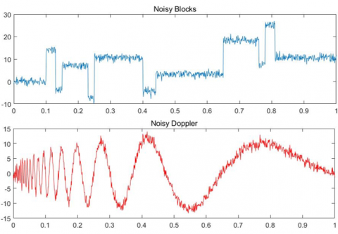
To disclose the influence of structural similarity on denoising effect, haar wavelet and sym8 smooth wavelet with vanishing moment of 8 were adopted to perform thresholding on two 1D signals, namely, doppler signal and blocks signal. The signal-to-noise ratio (SNR) of the signals is 20. The hard threshold function was adopted, for the two signals are relatively simple without many details.
The two noisy signals are illustrated in Figure 1. It can be seen that the doppler signal is a smooth curve, while the blocks signal consists of several step edges. Figure 2 shows the wavelet function waveforms of haar wavelet and sym8 wavelet. Comparing Figures 1 and 2, it is easy to learn that haar wavelet has a similar structure to the blocks signal, while the doppler signal and sym8 wavelet are relatively smooth.
Table 1 lists the SNRs of the denoised signals obtained through thresholding of doppler signal and blocks signal by four different threshold selection methods. The results show that, for the relatively smooth doppler signal, the denoising effect of sym8 wavelet is always better than that of haar wavelet, under any of the four threshold selection methods; the exactly opposite results were observed for the blocks signal with relatively large singularity. Therefore, the wavelet structure has a greater impact on signal denoising than threshold selection. Moreover, the smooth wavelet with a high vanishing moment has a larger application scope than the unsmooth wavelet. The latter only applies to signals with high singularity. If applied to smooth signals, the unsmooth wavelet might cause a plunge in the SNR [9].
Figure 1. Noisy blocks and doppler signals
Figure 2. Haar (left) and sym8 (right) wavelet functions
Table 1. Wavelet thresholding of Doppler and Blocks signals
|
Threshold Wavelet SNR |
doppler signals |
Blocks signal |
||
|
Haar signal |
Sym8 signal |
Haar wavelet |
Sym8 wavelet |
|
|
Fixed threshold |
15.0811 |
25.9739 |
29.3399 |
22.8408 |
|
Unbiased likelihood estimation threshold |
21.0939 |
23.9615 |
23.3225 |
22.2165 |
|
Hybrid threshold |
19.6438 |
24.9749 |
26.555 |
23.6326 |
|
Minimax criterion threshold |
18.5175 |
25.6156 |
26.3144 |
24.0433 |
2.2 Influence of orthogonality and bi-orthogonality on denoising effect
Besides structural similarity, the denoising effect is greatly affected by other wavelet features, such as orthogonality and bi-orthogonality, the order of vanishing moment, and the odd or even symmetry of high-pass wavelet filter [10-12].
Orthogonal wavelets have minimal correlations between the wavelet coefficients within and between the scales after decomposition. However, haar wavelet is the only orthogonal wavelet that obeys symmetry, i.e. having linear phase features. The image obtained by wavelet decomposition is a wavelet series, which is the result of a linear filtering. If the wavelet filter has a linear phase or generalized linear phase, it is possible to fully reconstruct the original image [13-15]. Thus, no orthogonal wavelet except for haar wavelet boasts the capability of full reconstruction.
This problem can be solved by the construction of biorthogonal wavelet, which acquires linear phase features at the cost of some of its orthogonality. With symmetric features, the biorthogonal wavelet can preserve the edge information well in image decomposition, and fully reconstruct the original image. However, the decomposition process has a high redundancy, owing to the large correlation between the wavelet decomposition coefficients.
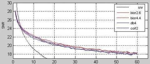
To disclose the influence of orthogonality and bi-orthogonality on denoising effect, both orthogonal wavelets (db4 and coif2) and biorthogonal wavelets (bior2.6 and bior4.4) were applied to denoise the same image. The global hard threshold function was adopted, with the decomposition scale of 2. The target image is an airplane image with additive zero-mean Gaussian white noises of different variances. The variance of the noise increased from 0.01 to 0.173 at the step length of 0.0224. The corresponding SNR changed from 35 to 10.
According to the SNR-variance curves after thresholding by orthogonal and biorthogonal wavelets (Figure 3), the SNR curves of the two orthogonal wavelets db4 and coif2 were very close to each other; the two biorthogonal wavelets achieved higher SNRs than the two orthogonal wavelets. The SNR-variance curves also indicate that biorthogonal wavelet outperforms orthogonal wavelet in denoising, in addition to its abilities of full reconstruction and edge preservation.
Figure 3. The SNR-variance curves after thresholding by orthogonal and biorthogonal wavelets
2.3 Influence of vanishing moment features on denoising effect
Apart from orthogonality and bi-orthogonality, the symmetry and vanishing moment also have important impacts on the wavelet denoising effect. The vanishing moment largely determines the smoothness of the wavelet. In general, wavelets with higher-order vanishing moments are smoother than those with lower-order vanishing moments. Furthermore, with the growing vanishing moment, more and more detail coefficients of wavelet decomposition approach zero, facilitating the localization of abrupt information like image edges. Of course, if the vanishing moment is too high, most of the high-frequency coefficients on the fine scale will also tend to zero, which weakens some information of the image [16].
Table 2 shows the SNRs of a noisy image after being denoised by db family wavelets db1~db10. The original image contains three levels of noises: 10, 15 and 20. Both soft and hard threshold functions were adopted in the denoising process. The data in Table 2 show that, for db family wavelets, hard thresholding is suitable for high noise level and soft thresholding for low noise level [17]. The vanishing moment should fall between 4 and 6, rather than take a very high value.
Table 2. Relationship between vanishing moment and SNR of db family wavelets
|
Wavelet |
db1 |
db2 |
db3 |
db4 |
db5 |
db6 |
db7 |
db8 |
db9 |
db10 |
|
|
Vanishing moment |
1 |
2 |
3 |
4 |
5 |
6 |
7 |
8 |
9 |
10 |
|
|
Soft thresholding SNR |
10 |
16.65 |
17.463 |
17.652 |
17.825 |
17.872 |
17.816 |
17.911 |
17.925 |
17.892 |
17.96 |
|
15 |
17.87 |
18.87 |
19.09 |
19.282 |
19.317 |
19.271 |
19.316 |
19.333 |
19.308 |
19.36 |
|
|
20 |
20.3 |
21.03 |
21.29 |
21.341 |
21.414 |
21.344 |
21.28 |
21.26 |
21.24 |
21.24 |
|
|
Hard thresholding SNR |
10 |
16.76 |
17.503 |
17.671 |
17.861 |
17.915 |
17.827 |
17.922 |
17.916 |
17.885 |
17.96 |
|
15 |
18.37 |
19.26 |
19.45 |
19.635 |
19.608 |
19.567 |
19.568 |
19.594 |
19.511 |
19.59 |
|
|
20 |
19.07 |
20.04 |
20.33 |
20.47 |
20.51 |
20.458 |
20.459 |
20.43 |
20.41 |
20.46 |
|
Table 3 shows the SNRs of a noisy image after being denoised by coif family wavelets coif1~coif5. The results demonstrate that, for coif family wavelets, the denoising effect was better under hard thresholding than under soft thresholding. Under the same vanishing moment, the SNRs obtained by coif family wavelets were better than those obtained by db family wavelets, through hard thresholding.
In addition, the coif family wavelets have approximately symmetry, which is not found in the db family wavelets. Therefore, the coif family wavelets can reconstruct the original image with a smaller error than the db family wavelets.
Table 3. Relationship between vanishing moment and SNR of coif family wavelets
|
Wavelet |
coif1 |
coif2 |
coif3 |
coif4 |
coif5 |
|
|
Vanishing moment |
2 |
4 |
6 |
8 |
10 |
|
|
Soft thresholding SNR |
10 |
17.525 |
17.846 |
17.932 |
17.966 |
17.985 |
|
15 |
18.916 |
19.311 |
19.405 |
19.441 |
19.46 |
|
|
20 |
20.04 |
20.46 |
20.548 |
20.572 |
20.586 |
|
|
Hard thresholding SNR |
10 |
17.571 |
17.888 |
17.97 |
18.017 |
18.029 |
|
15 |
19.263 |
19.635 |
19.689 |
19.711 |
19.717 |
|
|
20 |
21.069 |
21.401 |
21.518 |
21.487 |
21.497 |
|
2.4 Influence of waveform and odd or even symmetry of the decomposition end filter on denoising effect
The comparison between coif family wavelets and db family wavelets also shows the importance of symmetry in image denoising. There are two types of symmetry: odd symmetry and even symmetry. To disclose the influence of odd or even symmetry of high-pass decomposition filter, the bior family wavelets were selected to denoise a noisy airplane image. The SNRs of the denoised image were computed, and used to evaluate the said influence [18-20].
First, four bior family wavelets were adopted to perform global thresholding of the noisy airplane image at the decomposition scale of 3. The wavelet symmetries and SNRs of the denoised image are recorded in Table 4. The initial SNR of the original image was set to 15 and 20, respectively.
As shown in Figure 4, the SNR curves of the denoised images obtained through soft thresholding and hard thresholding were of the same form, although the SNR of the original image changed from 15 to 20. For the odd-symmetric high-pass decomposition filter, the SNRs were relatively low at wavelets bior1.3 and bior3.3. In addition, the soft thresholding result was better than hard thresholding result at bior3.3. Overall, the hard thresholding had much better result than soft thresholding, due to the high level of initial noise. Judging by the parity of the high-pass decomposition filter, the SNRs obtained by even symmetric wavelets clearly outshined those obtained by odd symmetric wavelets, especially those of bior2.2 and bior6.8.
Figure 4. The SNR curves of the denoised image by bior family wavelets
Next, five bior family wavelets were adopted to hard thresholding of the noisy airplane image at the decomposition scale of 3. The initial SNR of the original image was set to 20. According to the denoising results of different bior family wavelets (Figure 5), the odd symmetric wavelet of high-pass decomposition could improve the SNR of the original image to a certain extent, but lost many details in the denoising process, making the reconstructed image unclear. With the growth in decomposition scale, many edges of the reconstructed image became blurry. Hence, even symmetric biorthogonal wavelet should be selected for high-pass decomposition filter, during the wavelet thresholding of images.
Figure 5. The SNR curves of the denoised image by hard thresholding of bior family wavelets (SNR=20)
Table 4. The SNRs of the denoised image by bior family wavelets
|
Wavelet |
bior1.3 |
bior2.2 |
bior3.3 |
bior4.4 |
bior5.5 |
bior6.8 |
|
Symmetry |
Odd symmetry |
Even symmetry |
Odd symmetry |
Even symmetry |
Odd symmetry |
Even symmetry |
|
SNR=15 hard thresholding |
20.8815 |
22.6693 |
19.5274 |
22.4725 |
21.4613 |
22.6251 |
|
SNR=15 soft thresholding |
19.5879 |
21.4057 |
21.9581 |
20.9503 |
20.333 |
21.3654 |
|
SNR=20 hard thresholding |
23.2618 |
25.238 |
23.391 |
24.9368 |
23.8632 |
25.1753 |
|
SNR=20 soft thresholding |
21.5684 |
23.2624 |
24.0116 |
22.6849 |
22.0757 |
22.0349 |
In the process of image denoising, the high-pass decomposition filter should have zero-point even symmetry. The low-pass decomposition filter should also be analyzed quantitatively [21]. If a wavelet has an even-symmetrical high-pass decomposition filter, then its low-pass decomposition filter must be symmetrically even at the zero point.
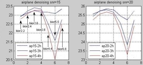
To analyze the abilities of the above wavelet families to retain low-frequency approximate information, the following biorthogonal wavelets, whose decomposition end filters are symmetrically even at the zero point, were adopted to denoise the airplane image: bior2.2, bior2.4, bior2.6, bior2.8, bior4.4, bior5.5 and bior6.8. Three decomposition scales were selected 2, 3, and 4. The initial SNR was set to 15 or 20. Figure 6 presents the SNR curves through hard thresholding under the above conditions.
It can be seen from Figure 6 that the decomposition-end filters of biorthogonal wavelets bior2.2, bior2.4, bior2.6 and bior2.8 exhibited the same behavior. These filters agree well in high-pass decomposition filter sequence, yet differ greatly in the length of low-pass decomposition filter sequence.
From the decomposition scale, when the low-pass decomposition filter is short, the SNR of the denoised image reduced greatly on the high-resolution scale (e.g. 4), indicating that shortening the sequence length will cause a severe loss of low-frequency information in the image. The growing decomposition scale improved the denoising effect, but the image reconstructed after denoising was not ideal.
Moreover, bior2.6 wavelet produced the best SNR on all decomposition scales, followed in turn by bior2.4, and bior2.2. Therefore, when the length of low-pass decomposition filter sequence falls in a certain range, the SNR is proportional to the sequence length. If the sequence is excessively long, the SNR cannot be further improved.
Comparing the results under the initial SNR of 15 with those under the initial SNR of 20, it can be seen that, when the noisy image has a high noise level (e.g. SNR=15), the denoising effect of decomposing scale 3 was way better than that of scale 2; when the noisy image has a low noise level (e.g. SNR=20), the denoising results of all wavelets were better on the single-scale than on the multi-scale, for the low-frequency information loss is alleviated by the reducing number of decomposition layers.
Figure 6. The SNR curves of biorthogonal wavelets with zero-point even-symmetrical decomposition end filters
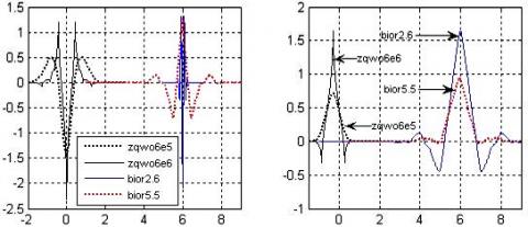
Figure 7 shows the decomposition-end filter waveforms of four wavelets bior2.6, bior5.5, zqwo6e5 and zqwo6e6. The latter two are a pair of wavelets obtained by parametric construction of FLTS biorthogonal wavelet. The two wavelets have the same initial scale factor, the same vanishing moment (1), and different values of the sign function. If the sign function is positive, the zqwo6e5 wavelet can be obtained; otherwise, the zqwo6e6 wavelet can be obtained.
Concerning high-pass decomposition filters, bior2.6, zqwo6e6 and zqwo6e5 all oscillated, with a negative peak. Among them, bior2.6 exhibited the best locality, followed by zqwo6e6; zqwo6e5 had the worst convergence. By contrast, bior5.5 wavelet also oscillated, but with a positive peak, and boasted the widest support.
Concerning low-pass decomposition filters, the waveforms of bior2.6 and zqwo6e6 were the most similar, and both attenuated rapidly. However, bior2.6 had a much wider support than zqwo6e6. The low-pass filter of bior5.5 was widely supported and oscillatory but attenuated slowly. Meanwhile, zqwo6e5 was not oscillatory and its decomposition scale function attenuated at the slowest rate.
Table 5 compares the SNRs of the airplane images denoised by the above four wavelets with the decomposition scales of 2 and 3 and the initial SNRs of 15 and 20. The hard thresholding and simple reconstruction were adopted for the denoising, aiming to reveal the abilities of the wavelets to retain low-frequency approximate information. The simple reconstruction refers to the reconstruction of a nosy image after setting all the detail coefficients to zero. Thus, the SNR of the denoised image only relates to the low-frequency approximation coefficient of the wavelet.
Figure 7. The decomposition-end filter waveforms of four wavelets bior2.6, bior5.5, zqwo6e5 and zqwo6e6
According to the data of simple reconstruction (Table 5), the increase of decomposition scale led to a serious loss of the approximate information of the image. Under the decomposition scale of 2, the SNR ratio of the simply reconstructed image was highly correlated with the noise level. The reconstruction results of each wavelet at SNR=20 were much better than those at SNR=15. This means, at a high noise level, the low-frequency approximation coefficients after the two-layer decomposition still carry a certain amount of noises. When the decomposition scale increased to 3, the initial SNR exerted no significant effect on the simply reconstructed image. Each wavelet had almost the same SNR of the reconstruction image, whether the initial SNR was 15 or 20. In other words, the noises have basically been separated from the approximate coefficients after the three-layer wavelet decomposition. In this case, if thresholding is performed, the SNR of the denoised image hinges on the denoising ability of the wavelet.
From the thresholding results, it can be seen that the SNRs of the images denoised by bior2.6 and zqwo6e6 increased faster than the SNRs of those denoised by other wavelets. In contrast, bior5.5 failed to achieve a satisfactory thresholding effect, despite its good ability in retaining low-frequency information. Hence, bior5.5 has a poor noise separation ability.
Table 5. The SNRs of the airplane image denoised by the four wavelets (N: decomposition scale)
|
Wavelet |
SNR=15 N=2 |
SNR=15 N=3 |
SNR=20 N=2 |
SNR=20 N=3 |
||||
|
Zero-setting |
Denoising |
Zero-setting |
Denoising |
Zero-setting |
Denoising |
Zero-setting |
Denoising |
|
|
bior2.6 |
22.493 |
23.2403 |
18.5688 |
23.4053 |
23.6912 |
25.8429 |
18.6643 |
25.7905 |
|
bior5.5 |
22.8175 |
23.08 |
18.9707 |
21.5624 |
24.1752 |
25.226 |
19.0077 |
23.8354 |
|
zqwo6e5 |
12.6756 |
16.2966 |
6.2448 |
15.8144 |
13.0849 |
20.744 |
6.3099 |
20.1436 |
|
zqwo6e6 |
21.9776 |
22.3119 |
18.1279 |
22.1605 |
23.0318 |
24.8075 |
18.2175 |
24.4207 |
The following conclusions can be drawn from the waveforms of the decomposition end filters of wavelets:
In wavelet thresholding, the low-pass decomposition filter should have attenuating oscillation. The wavelet with a wide support interval can effectively retain the approximate information of the image. Both orthogonal wavelet and biorthogonal wavelet could suppress image noise and enhance the SNR, but the biorthogonal wavelet has the better performance, for its linear phase features prevent the visual distortion of the reconstruction image. A high vanishing moment is not necessarily favorable for image denoising; if the vanishing moment is too high, the detail coefficients of wavelet decomposition will approach zero, and the reconstructed images after thresholding will have blurry edges and a low SNR. For biorthogonal wavelets, the odd or even symmetry of high-pass decomposition filter has a great impact on the decomposition coefficients.
To sum up, the most desirable wavelet for image denoising is the biorthogonal wavelet, in which the decomposition end filter has zero point even symmetry, the low-pass decomposition filter is oscillatory with a wide support interval, and the high-pass decomposition filter has a short support and attenuates fast.
3.1 Wavelet construction
To achieve the optimal performance, our wavelet was designed by parametric construction of FLTS biorthogonal wavelet [22]. Suppose the high-pass decomposition filter is 3 in length and even-symmetric at the zero point. Then, the high-pass decomposition $\tilde{g}$ and the low-pass reconstruction filter h can be expressed as:
$\tilde{g}=\left\{\tilde{g}_{0}, \tilde{g}_{1}, \tilde{g}_{2}\right\}$ and $h_{k}=(-1)^{k-1} \tilde{g}_{1-k} h=\left\{h_{-1}, h_{0}, h_{1}\right\}$
According to the conditional relationship of filters, we have:
$h=\left\{\frac{\sqrt{2}}{4}, \frac{\sqrt{2}}{2}, \frac{\sqrt{2}}{4}\right\} \tilde{g}=\left\{\frac{\sqrt{2}}{4},-\frac{\sqrt{2}}{2}, \frac{\sqrt{2}}{4}\right\}$
Under the limitation of the odd-length filter, if the h is 3 in length, then the length N of the low-pass decomposition filter $\tilde{h}$ must satisfy that N+1 is not an integer multiple of 4. In other words, if the sequence length of $\tilde{h}$ is 7, 11, 15…, the wavelet to be constructed does not exist [23]. Let the sequence length of the low-pass decomposition filter $\tilde{h}$ be 13, we have:
$\tilde{h}=\left\{\tilde{h}_{-6}, \cdots, \tilde{h}_{-1}, \tilde{h}_{0}, \tilde{h}_{1}, \cdots, \tilde{h}_{6}\right\}$$\underrightarrow{{ Even symmetry }}\left\{\tilde{h}_{6}, \cdots, \tilde{h}_{1}, \tilde{h}_{0}, \tilde{h}_{1}, \cdots, \tilde{h}_{6}\right\}$
To adjust the attenuation of the low-pass decomposition filter $\tilde{h}$, a scale factor k was introduced such that:
$\tilde{h}_{0}=k \tilde{h}_{1} \quad k>0$
According to the conditional relationship of the filter and the PR relationship of full reconstruction, the construction relation equations of the biorthogonal wavelet with the filter length (13-3) at the decomposition end can be derived as:
$\left\{\begin{aligned} \tilde{h}_{0}+2\left(\tilde{h}_{2}+\tilde{h}_{4}+\tilde{h}_{6}\right) &=\frac{\sqrt{2}}{2} \\ \tilde{h}_{1}+\tilde{h}_{3}+\tilde{h}_{5} &=\frac{\sqrt{2}}{4} \\ \frac{\sqrt{2}}{4} \tilde{h}_{1}+\frac{\sqrt{2}}{2} \tilde{h}_{0}+\frac{\sqrt{2}}{4} \tilde{h}_{1} &=1 \\ \frac{\sqrt{2}}{4} \tilde{h}_{1}+\frac{\sqrt{2}}{2} \tilde{h}_{2}+\frac{\sqrt{2}}{4} \tilde{h}_{3} &=0 \\ \frac{\sqrt{2}}{4} \tilde{h}_{3}+\frac{\sqrt{2}}{2} \tilde{h}_{4}+\frac{\sqrt{2}}{4} \tilde{h}_{5} &=0 \\ \frac{\sqrt{2}}{4} \tilde{h}_{5}+\frac{\sqrt{2}}{2} \tilde{h}_{6}=0 \end{aligned}\right.$$\underrightarrow{\widetilde{n}_{0}=k \widetilde{h}_{1}}$$\left\{\begin{array}{c}{k \tilde{h}_{1}+2\left(\tilde{h}_{2}+\tilde{h}_{4}+\tilde{h}_{6}\right)=\frac{\sqrt{2}}{2}} \\ {\tilde{h}_{1}+\tilde{h}_{3}+\tilde{h}_{5}=\frac{\sqrt{2}}{4}} \\ {\tilde{h}_{1}=\frac{\sqrt{2}}{k+1}} \\ {\tilde{h}_{1}+2 \tilde{h}_{2}+\tilde{h}_{3}=0} \\ {\tilde{h}_{3}+2 \tilde{h}_{4}+\tilde{h}_{5}=0} \\ {\tilde{h}_{5}=-2 \tilde{h}_{6}}\end{array}\right.$ (1)
The attenuation speed at the center of the low-pass decomposition filter $\tilde{h}$ can be changed by adjusting the scale factor k. According to the condition of vanishing moment, the m-th order of the vanishing moment can be obtained if:
$\left\{\begin{array}{l}{\tilde{h}_{0}-2 \tilde{h}_{1}+2 \tilde{h}_{2}-2 \tilde{h}_{3}+2 \tilde{h}_{4}-2 \tilde{h}_{5}+2 \tilde{h}_{6}=0} \\ {-\tilde{h}_{1}+2^{j} \tilde{h}_{2}-3^{j} \tilde{h}_{3}+4^{j} \tilde{h}_{4}-5^{j} \tilde{h}_{5}+6^{j} \tilde{h}_{6}=0}\end{array}\right.$$0<j<m$ j is an even number (2)
The parametric expressions of the biorthogonal wavelet with the m-th order vanishing moment and zero point even symmetry can be derived from formulas (1) and (2). If m=2 and k=1, 2 or 4, the three biorthogonal wavelets obtained have the same high-pass decomposition filter. Meanwhile, the low-pass decomposition filters can be expressed as:
$k=1 \quad d l=\{-0.0718,0.1436,0.1768,-0.4972,-0.1050,0.7071,0.7071, \cdots,-0.0718\}$
$k=2 \quad d l=\{-0.0203,0.0405,0.0589,-0.1584,-0.1565,0.4714,0.9428 \cdots,-0.0203\}$
$k=4 \quad d l=\{0.0343,-0.0685,-0.0354,0.1392,-0.2110,0.2828,1.1314, \cdots, 0.0343\}$
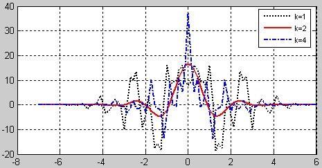
Figure 8. Waveforms of the three low-pass decomposition filters of the wavelet at different scale factors
Figure 8 shows the waveforms of the three low-pass decomposition filters of the wavelet. As shown in Figure 8, when k=1, the dual scale function of the constructed wavelet had poor convergence, which oscillated violently rather than attenuate in most of the support interval. This means the constructed wavelet has very poor locality. When k=4, the attenuation of the dual scale function was greatly improved, especially the localization ability. However, the function was not smooth in this case. By contrast, when k=2, the dual scale function of the constructed scale enjoyed good attenuation features and high smoothness.
Table 6 shows the global hard thresholding results of the three wavelets with second-order vanishing moments constructed at k=1, 2 and 4 on the missile image. The decomposition scales were set to 2, 3 and 4, in turn, and the initial SNRs were set to 15 and 25. The SNRs in the table show that, when k=1, the constructed wavelets were basically unable to suppress image noise. When the initial SNR was high, the denoising could not greatly improve the SNR; when the initial SNR was low, the denoising reduced the image quality. When k=4, the constructed wavelets had a certain denoising ability, and improved the SNR of the noisy image under both initial SNRs. When k=2, the constructed wavelets achieved the best denoising effects, showing excellent attenuation and smoothness features.
From the relationship between SNR and decomposition scale, it is learned that the SNR decreased, as the decomposition scale increased further from 2. Hence, the wavelets with second-order vanishing moment cannot detect the highly singular points. The noises with large singularities in the decomposition detail coefficients cannot be separated effectively.
Table 6. The SNRs of the images denoised by wavelet thresholding at the vanishing moment of 2 and different scale factors
|
Initial condition Constructed wavelet |
Initial SNR=15 |
Initial SNR=25 |
||||
|
N=2 |
N=3 |
N=4 |
N=2 |
N=3 |
N=4 |
|
|
k=1 |
17.3667 |
16.6902 |
16.4669 |
24.3188 |
23.7421 |
23.5604 |
|
k=2 |
22.8442 |
23.206 |
23.0617 |
27.2328 |
27.0348 |
26.9243 |
|
k=4 |
21.1013 |
20.8559 |
21.0633 |
26.3372 |
26.0678 |
25.9785 |
To further improve the denoising ability of the constructed wavelet, the vanishing moment features were optimized at the scale factor of 2. When the vanishing moment increased from 2 to 4, the relationship of the vanishing moment of the wavelet to be constructed can be expressed as:
$\left\{\begin{array}{ll}{\tilde{h}_{1}=4 \tilde{h}_{2}-9 \tilde{h}_{3}+16 \tilde{h}_{4}-25 \tilde{h}_{5}+36 \tilde{h}_{6}} & {m=2} \\ {\tilde{h}_{1}=16 \tilde{h}_{2}-81 \tilde{h}_{3}+256 \tilde{h}_{4}-625 \tilde{h}_{5}+1296 \tilde{h}_{6}} & {m=4}\end{array}\right.$ (3)
From formulas (1) and (3), the low-pass decomposition filter at the vanishing moment of 4 can be derived as:
$d l=\{-0.0091,0.0181,0.0589,-0.1360$, $-0.1677,0.4714,0.9428 \cdots,-0.0091\}$
Similarly, the low-pass decomposition filter at the vanishing moment of 6 can be constructed as:
$d l=\{-0.0042,0.0084,0.0589,-0.1263$, $-0.1726,0.4714,0.9428 \cdots,-0.0042$
For simplicity, the wavelets of the second-, fourth- and sixth- order vanishing moments obtained at k=2 are denoted as zqwo6e12, zqwo6e14 and zqwo6e16, respectively.
3.2 Self-adaptive hierarchical thresholding algorithm
During image thresholding, the global thresholding cannot retain image details while effectively removing noises [24, 25]. Theoretically speaking, the hierarchical thresholding can strike a balance between noise suppression and detail preservation.
Let m be the decomposition scale, thr be the initial threshold, and k be the current number of decomposition layers. The hierarchical thresholding algorithm can be implemented as follows:
Step 1. Obtain the approximate coefficients $\{a\}_{k}$ and detail coefficient of each layer through wavelet transform, $1 \leq k \leq n$;
Step 2. Calculate and normalize the energy of the detail coefficient of each layer, and derive the variance of the normalized detail coefficient sequence std$_{-} d_{k} 1 \leq k \leq n$;
Step 3. Compute the threshold value at each scale by the hierarchical threshold relationship:
$\operatorname{th} r_{k}=\frac{s t d_{-} d_{1}}{s t d_{-} d_{k}} \times t h r$
Step 4. Perform soft or hard thresholding of the detail coefficients at each scale, using the hierarchical threshold $t h r_{k}$.
Step 5. Reconstruct the post-thresholding coefficients to obtain the denoised results.
The self-adaptive hierarchical threshold algorithm can adaptively select the proportional relationship between thresholds of different scales for the denoising process, according to the noise level of the original image and the attenuation speed of the noises.
This section aims to evaluate the noise suppression ability of the constructed wavelet and verify the self-adaptive hierarchical thresholding algorithm. Specifically, six biorthogonal wavelets were adopted for thresholding a noisy image called smallplane. The image is a simple photo of a flying plane taken from the distance. The six wavelets are all even symmetric at the zero point, including zqwo6e12, zqwo6e14, zqwo6e16 and bior5.5, bior2.6 and bior4.4.
Table 7 shows the global thresholding results of the smallplane image at the decomposition scale of 2-5 and the initial SNRs of 15 and 20, and Table 8 presents the results of self-adaptive hierarchical thresholding on the same image.
Through global thresholding, the SNR obtained by every wavelet decreased with the growth in decomposition scale, due to the erroneous deletion of detail coefficients. bior5.5 had the fastest decline in denoising quality, revealing an extremely poor ability to retain low-frequency approximation information. Through self-adaptive hierarchical thresholding, the image details were preserved well, as the threshold of each scale was adjusted. As a result, the SNR obtained by self-adaptive hierarchical thresholding was much better than that of global thresholding. As shown in Table 8, the SNRs obtained by bior5.5 and bior2.2, which had poor denoising effects through global thresholding on large decomposition scales, did not decrease, but remained on a high level. By contrast, the other four wavelets achieved better denoising effects. When the decomposition scale was not greater than 4, the SNR of the denoised image through self-adaptive hierarchical thresholding increased with the scale.
Table 7. Global thresholding results of smallplane image
|
Initial condition Wavelet |
Initial SNR=15 |
Initial SNR=25 |
||||||
|
N=2 |
N=3 |
N=4 |
N=5 |
N=2 |
N=3 |
N=4 |
N=5 |
|
|
bior5.5 |
24.59 |
24.2 |
22.5 |
21.63 |
26.98 |
25.26 |
24.17 |
23.77 |
|
bior2.6 |
24.66 |
25.17 |
24.74 |
24.45 |
27.24 |
27.07 |
26.75 |
26.75 |
|
bior2.2 |
24.47 |
25.01 |
24.76 |
24.47 |
26.99 |
26.77 |
26.55 |
26.4 |
|
zqwo6e12 |
24.62 |
25.2 |
24.8 |
24.51 |
27.24 |
27.05 |
26.88 |
26.76 |
|
zqwo6e14 |
24.61 |
25.14 |
24.79 |
24.51 |
27.23 |
27.11 |
26.87 |
26.73 |
|
zqwo6e16 |
24.59 |
25.12 |
24.77 |
24.48 |
27.22 |
27.1 |
26.86 |
26.73 |
Table 8. Self-adaptive hierarchical thresholding results of smallplane image
|
Initial condition Wavelet |
Initial SNR=15 |
Initial SNR=25 |
||||||
|
N=2 |
N=3 |
N=4 |
N=5 |
N=2 |
N=3 |
N=4 |
N=5 |
|
|
bior5.5 |
24.63 |
25.72 |
25.68 |
25.7 |
27.4 |
27.6 |
27.67 |
27.63 |
|
bior2.6 |
24.28 |
24.78 |
24.67 |
24.68 |
27.51 |
27.77 |
27.86 |
27.83 |
|
bior2.2 |
23.8 |
23.914 |
23.912 |
23.911 |
27.24 |
27.28 |
27.27 |
27.27 |
|
zqwo6e12 |
24.13 |
24.59 |
24.55 |
24.51 |
27.4 |
27.69 |
27.74 |
27.66 |
|
zqwo6e14 |
24.15 |
24.64 |
24.56 |
24.54 |
27.42 |
27.71 |
27.75 |
27.71 |
|
zqwo6e16 |
24.14 |
24.61 |
24.54 |
24.54 |
27.43 |
27.71 |
27.73 |
27.73 |
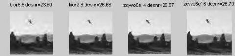
Figures 9 and 10 display the denoising results of the global thresholding and self-adaptive hierarchical thresholding on the smallplane image at the initial SNR of 20 and decomposition scale of 5, respectively. It can be seen that the self-adaptive hierarchical thresholding achieved a much higher SNR and retained more edge details than the global thresholding. The advantages are most obvious in the results of bior5.5. In the denoised image by global thresholding, there are obvious ringing artefacts, and the edges of the smallplane are completely blurred.
Figure 9. Global thresholding results of smallplane image (initial SNR=20)
Figure 10. Self-adaptive thresholding results of smallplane image (initial SNR=20)
This paper proves that the three wavelets obtained by the parametric construction of FLTS biorthogonal wavelet have good denoising ability facing various noise levels, large decomposition scales, and images of different complexities. Comparing the SNRs obtained by the three wavelets, it is concluded that the vanishing moment should be controlled at a moderate level if the target image is relatively simple, and the vanishing moment should be relatively high if the target image is complex. The author also compared the denoising effects of global thresholding and self-adaptive hierarchical thresholding. The comparison shows that the self-adaptive hierarchical thresholding is less dependent on the wavelet features, more adaptable to different types of images, and better in denoising ability. In particular, the self-adaptive hierarchical thresholding can preserve the edges of the target image excellently under a high decomposition scale.
The authors were endowed by water conservancy science and technology project of Shaanxi Province (2019slkj-19).
[1] Ansari, R.A., Buddhiraju, K.M. (2017). A comparative evaluation of denoising of remotely sensed images using wavelet, curvelet and contourlet transforms. Journal of the Indian Society of Remote Sensing, 45(1): 193-193. https://doi.org/10.1007/s12524-016-0579-0
[2] Ansari, R.A., Budhhiraju, K.M. (2016). A comparative evaluation of denoising of remotely sensed images using wavelet, curvelet and contourlet transforms. Journal of the Indian Society of Remote Sensing, 44(6): 843-853. https://doi.org/10.1007/s12524-016-0552-y
[3] Aravindan, T.E., Seshasayanan, R. (2018). Denoising brain images with the aid of discrete wavelet transform and monarch butterfly optimization with different noises. Journal of Medical Systems, 42(11): 207. https://doi.org/10.1007/s10916-018-1069-4
[4] Bascoy, P.G., Quesada-Barriuso, P., Heras, D.B., Arguello, F. (2019). Wavelet-based multicomponent denoising profile for the classification of hyperspectral images. Ieee Journal of Selected Topics in Applied Earth Observations and Remote Sensing, 12(2): 722-733. https://doi.org/10.1109/jstars.2019.2892990
[5] Bhandari, A.K., Kumar, D., Kumar, A., Singh, G.K. (2016). Optimal sub-band adaptive thresholding-based edge preserved satellite image denoising using adaptive differential evolution algorithm. Neurocomputing, 174: 698-721. https://doi.org/10.1016/j.neucom.2015.09.079
[6] Biswas, M., Om, H. (2016). A new adaptive image denoising method based on neighboring coefficients. Journal of the Institution of Engineers (India): Series B (Electrical, Electronics & Telecommunication and Computer Engineering), 97(1): 11-19. https://doi.org/10.1007/s40031-014-0166-0
[7] Bouhali, A., Berkani, D. (2017). Combination of spatial filtering and adaptive wavelet thresholding for image denoising. International Journal of Image, Graphics and Signal Processing, 9(5): 9-19. https://doi.org/10.5815/ijigsp.2017.05.02
[8] Diwakar, M., Kumar, M. (2018). A review on CT image noise and its denoising. Biomedical Signal Processing and Control, 42: 73-88. https://doi.org/10.1016/j.bspc.2018.01.010
[9] Farfuq, S.K.U., Ramanaiah, K.V., Rajan, K.S. (2012). A novel algorithm for generalized image denoising using dual tree complex wavelet transform. i-Manager's Journal on Software Engineering, 7(2): 24-33.
[10] Farouj, Y., Freyermuth, J.M., Navarro, L., Clausel, M., Delachartre, P. (2017). Hyperbolic wavelet-fisz denoising for a model arising in ultrasound imaging. Ieee Transactions on Computational Imaging, 3(1): 1-10. https://doi.org/10.1109/tci.2016.2625740
[11] Goyal, B., Agrawal, S., Sohi, B.S., Dogra, A. (2016). Noise reduction in MR brain image via various transform domain schemes. Asian Journal of Research in Chemistry, 9(7): 919-924. https://doi.org/http://dx.doi.org/10.5958/0974-360X.2016.00176.1
[12] Kamble, V.M., Parlewar, P., Keskar, A.G., Bhurchandi, K.M. (2016). Performance evaluation of wavelet, ridgelet, curvelet and contourlet transforms based techniques for digital image denoising. Artificial Intelligence Review, 45(4): 509-533. https://doi.org/10.1007/s10462-015-9453-7
[13] Khmag, A., Ramli, A.R., Kamarudin, N. (2019). Clustering-based natural image denoising using dictionary learning approach in wavelet domain. Soft Computing, 23(17): 8013-8027. https://doi.org/10.1007/s00500-018-3438-9
[14] Kumar, S., Sarfaraz, M., Ahmad, M.K. (2018). Denoising method based on wavelet coefficients via diffusion equation. Iranian Journal of Science and Technology Transaction a-Science, 42(A2): 721-726. https://doi.org/10.1007/s40995-017-0228-7
[15] Lu, Z., Pei, D. (2016). Algorithm of image denoising based on the optimized method of wavelet thresholding. Audio Engineering, 40(4): 39-44. https://doi.org/10.16311/j.audioe.2016.04.09
[16] Rabbouch, H., Saadaoui, F. (2018). A wavelet-assisted subband denoising for tomographic image reconstruction. Journal of Visual Communication and Image Representation, 55: 115-130. https://doi.org/10.1016/j.jvcir.2018.05.004
[17] Remenyi, N., Nicolis, O., Nason, G., Vidakovic, B. (2014). Image denoising with 2D scale-mixing complex wavelet transforms. Ieee Transactions on Image Processing 23(12): 5165-5174. https://doi.org/10.1109/tip.2014.2362058
[18] Saravani, S., Shad, R., Ghaemi, M. (2018). Iterative adaptive Despeckling SAR image using anisotropic diffusion filter and Bayesian estimation denoising in wavelet domain. Multimedia Tools and Applications, 77(23): 31469-31486. https://doi.org/10.1007/s11042-018-6153-8
[19] Shi, S., Qu, S.R., Zhao, H., Chen, F.L. (2012). A line enhancement algorithm for infrared image based on ridgelet. Applied Mechanics and Materials, 182: 1786-1790. https://doi.org/http://dx.doi.org/10.4028/www.scientific.net/AMM.182-183.1786
[20] Suryanarayana, G., Dhuli, R. (2016). Shock filter-based image super-resolution using dual-tree complex wavelet transform and singular value decomposition. Compel, 35(3): 1162-1178.
[21] Talbi, M., Bouhlel, M.S., Cherif, A. (2017). A hybrid technique of image denoising using the curvelet transform based denoising method and two-stage image denoising by PCA with local pixel grouping. Current Medical Imaging Reviews, 13(4): 484-494. https://doi.org/10.2174/1573405613666170614082754
[22] Vijayaraghavan, V., Karthikeyan, M. (2018). Denoising of images using principal component analysis and undecimated dual tree complex wavelet transform. International Journal of Biomedical Engineering and Technology, 26(3-4): 304-315.
[23] Wang, Y., Lei, F., Fu, G.J. (2013). Adaptive denoising algorithms based on wavelet for pool underwater image. Applied Mechanics and Materials, 333: 1024-1029. https://doi.org/http://dx.doi.org/10.4028/www.scientific.net/AMM.333-335.1024
[24] Zhao, H.H., Jr, J.F.L., Martinez, A., Qiao, Z.J. (2013). SAR image denoising based on wavelet packet and median filter. Applied Mechanics and Materials, 333: 916-919. https://doi.org/http://dx.doi.org/10.4028/www.scientific.net/AMM.333-335.916
[25] Zhong, Y.F., Fu, L.J., Zhou, T. (2012). Based on median pyramid transform of the color image inverse halftoning. Applied Mechanics and Materials, 200: 724-729. https://doi.org/http://dx.doi.org/10.4028/www.scientific.net/AMM.200.724