Gottumukkala HimaBindu* | Chinta Anuradha | Patnala S.R. Chandra Murty
© 2019 IIETA. This article is published by IIETA and is licensed under the CC BY 4.0 license (http://creativecommons.org/licenses/by/4.0/).
OPEN ACCESS
The aim of the work is to identify the duplication in a video database with the aid of feature extraction techniques. The process includes extraction of image features (shape, color, and texture) for duplicate identification. The color contains 256 features, shape contains 200 features, the texture contains two different features namely gray-level co-occurrence matrix (GLCM) (22 features in 4 degrees) and grey-level run length matrix (GLRLM) (11 features) are extracted. In this paper, the preliminary work is to convert video into frames and then each frame into blocks subsequently including feature extraction. A query video is then considered for the same process of feature extraction and compared with the normal video. The distance between query video and normal video if found to be similar then the video identified as duplicate video. The results are performed for various evaluation matrix and plotted graphs are shown. The sensitivity value for whole feature extractions is 0.88, the specificity value for whole feature extractions is 0.83 and the accuracy value for whole extractions is 0.86. The entire process implemented in the working platform of MATLAB.
video, shape, color, grey-level co-occurrence matrix (GLCM), grey-level run length matrix (GLRLM)
With the on-going advances in low-cost multimedia devices and digital communication technologies, vast amounts of video content would be able to be caught, stored, and transmitted through the internet each day [1]. The number of online videos has encountered an exponential development in current decades, particularly when social video sharing sites came into existence [2]. The techniques involved in digital video forensics fall under two classes namely active and passive. The approaches in the main class implant a watermark, uniquely made, in the video while it is generated and the later does not require any authentication for the information [3]. Subsequently there is also a requirement of significant measure for compressing the videos due to cost-effective storage and bandwidth limitation [4]. Thereby an issue is exacerbated on account of the video because of its impressively huge volume (contrasted with content and images), which make it an extraordinary test for each web-based video platform as well as for systems that analyze and list a lot of web video content [5]. A video format can be expected as a sequence of images namely frames, considered over a period of time, whereby the tampering detection methods produced for image forensics [6-10] could be connected at the frame level. The feature vectors encode the properties of the image, so as to be specific color, texture, and shape. The comparison among two images is figured as a function of the distance between their feature vectors [11]. In the spatial area, an extensively used feature extraction technique forms the spatial gray-level co-occurrence matrix (GLCM) from which a great deal of the second-order statistics could be resolved and examined and also textural features can likewise be extracted from the spectral domains namely frequency domain, wavelet domain, and Gabor domain [12]. Texture investigation and examination assume a fundamental job in many image processing applications [13]. The trained system when provided with a query image retrieves and demonstrates the images which are similar and relevant to the query considered from the database [14]. Finally the work in the paper aims at developing a successful plan for detecting and localizing duplicates in videos [15].
Soumya Prakash Rana et al. [16] 2019, had anticipated an image was incomprehensible by a single feature. Thereby the examination keeps an eye on the point of content-based image retrieval (CBIR) by joining the non-parametric texture feature with the parametric color and shape features. Finally, a hypothesis test was done to set up the implication of the proposed work that induces the assessed true values of precision and recall and acknowledging all in the image database.
Taşci [17] 2018, had planned to maintain images in the large databases, extracting useful information from the images and retrieval comparable images are the rising exploration region in the current situation. That feature can be used for solving various issues, for instance, reducing the dimension of the image, classifying the images, indexing the images in the image database, automatic data analysis and retrieval of images from the database, and so on.
Fudong Nian et al. [18] 2017, had anticipated a video characteristic portrayal learning algorithm for conception of video concept and used the educated explicit video attribute to improve the video captioning performance. Experimental outcomes on video captioning tasks demonstrate that the proposed technique, using just the
Jianmei Yang et al. [19] 2016, had proposed a method of duplicating the chosen frames from a video to another area within a similar video form a standout amongst the most common methods of video forgery. The experimental results demonstrate that their algorithm proposed gives detection accuracy which yields higher values than the previous existing algorithms, and proves to have an outstanding performance in the terms of time efficiency.
Vivek Kumar Singh and R.C. Tripathi [20] 2011, had planned to wipe out or incorporate a definite amount of data on the images mainly for the assurance of specific forgery. The focus of the paper was to identify “copy move” kind of forgery. The method includes, reordering of one portion of the image somewhere else in the comparative image. The motivation behind this sort of image forgery was to hide certain significant features from the original image. In the paper, they intend a technique which was extra successful and reliable rather than prior methods.
The purpose of our work is to identify the duplication in a video database with the aid of features. To pursue this objective, preliminary work includes converting video into frames and then into blocks. Further work includes image feature extraction (shape, color, and texture) for duplicate identification. The color contains 256 features, shape contains 200 features, the texture contains two different features namely GLCM (22 features in 4 degrees) and GLRLM (11 features). Subsequently, a query video is taken for features extraction and compared with the normal video, if the distance between query video and normal video is found to be similar then the video is identified as duplicate. The results are performed for various evaluation matrix and plotted graphs are shown.
3.1 Video to frame conversion
To perform the work the video cannot be directly utilized for identification. The process includes converting of video into image frames and further converting them into blocks so as to retrieve accurate predicting rate feature extraction which plays a significant role.
3.2 Feature extraction
The images subsequent to frames and the feature extracted by a method for adjusting shape, color, texture (GLCM and GLRLM) in the feature extraction process.
3.2.1 Shape feature extraction
The shape is a fundamental source of data which is utilized for object recognition. Without shape, the visual content of the object cannot be recognized properly. Image is incomplete without recognizing the shape feature. In this mathematical morphology, a method is utilized that gives a way to deal with digital images which depends on the shape. Properly utilized, mathematical morphological operations tend to extract their basic shape attributes and wipe out irrelevancies.
3.2.2 Color feature extraction
Color space represents the color in the form of intensity value. We can specify, visualize and create the color with the help of the colorspace method. There exist many dissimilar color feature extraction methods.
Color histogram. The color histogram represents the image from an alternate point of view. The image in which color bins of the frequency distribution are represented by color histogram counts the pixels which are comparative and store it. Color histogram analyzes every statistical color frequency in an image. The change which happens in the translation, rotation, and angle of view are the issues solved by color histogram and furthermore, it focuses on individual parts of an image. The computation of local color histogram is simple and it is impervious to minor variations in the image for indexing and retrieval of image database, thus proved to be imperative.
3.2.3 Texture feature extraction
The texture contains critical data about the fundamental arrangement of the surface such as clouds, leaves, bricks, fabric, etc. It additionally defines surface with environment relationship. Texture feature additionally depicts the physical composition of the surface. There are many diverse techniques of texture feature extraction
Grey-level co-occurrence matrix (GLCM). A GLCM always signifies a matrix in which the no. of rows and columns are proportionate to the no. of combination of gray levels with value G, in the image. The matrix element p (u,v/d1,d2) symbolizes the identical isolation through a pixel separation (d1 and d2) . The GLCMs are arranged for get-together suitable valuations by a method of greycoprops function, which ensemble the insights with respect to the texture of an image, that is set in the below section.
Each feature implies the texture uniformity and non-uniformity, similarity, dissimilarity and different parameters. The Angular Second Moment or Energy signifies the uniformity in the image and is calculated utilizing equation (8) where p (u,v) is the pixel value at the point u,v of the texture image which is of size (MXN). The entropy chooses the dispersal change in the image. It is a proportion of non-consistency and is assessed by the equation (9). The homogeneity estimates the consistency of the non-zero areas in GLCM. As the grey values are higher, lower, GLCM homogeneity, thus reassuring an unrivalled GLCM contrast. The homogeneity is inside scope of [0, 1]. On the off chance that the image is simply sufficiently varied, at that point the homogeneity is more unmistakable and if the image is not in any way changed, at that point the homogeneity becomes equivalent to one. The features considered for GLCM are
$Autocorrelation=\,\,\,\,\sum\limits_{v}{\sum\limits_{u}{uvp(u,v)}}\,(1)$ (1)
$Contrast\,=\,\,\,\,\sum\limits_{v}{\sum\limits_{u}{{{(u-v)}^{2}}}}\,p(u,v)$ (2)
$Correlation1=\,\,\,\,\sum\limits_{v}{\sum\limits_{u}{\frac{(u-{{m}_{u}})(v-{{m}_{v}})p(u,v)}{{{\sigma }_{u}}{{\sigma }_{v}}}}}\,(3)$ (3)
$Correlation2=\,\,\,\,\sum\limits_{v}{\sum\limits_{u}{\frac{(uvp(u,v)-{{m}_{u}}{{m}_{v}})}{{{\sigma }_{u}}{{\sigma }_{v}}}(4)}}\,$ (4)
$Cluster\Pr o\min ence=\,\,\,\,\sum\limits_{u}{\sum\limits_{v}{{{((u-{{m}_{u}})+(v-{{m}_{v}}))}^{4}}p(u,v)}}$ (5)
$ClusterShade=\,\,\,\,\sum\limits_{u}{\sum\limits_{v}{{{((u-{{m}_{u}})+(v-{{m}_{v}}))}^{3}}p(u,v)}}$ $ClusterShade=\,\,\,\,\sum\limits_{u}{\sum\limits_{v}{{{((u-{{m}_{u}})+(v-{{m}_{v}}))}^{3}}p(u,v)}}$ (6)
$Dissimilarity=\sum\limits_{u}{\sum\limits_{v}{|u-v|p(u,v)}}\,\,$ (7)
$Energy=\sum\limits_{u}{\sum\limits_{v}{p{{(u,v)}^{2}}}}\,\,$ (8)
$Entrop{{y}^{{}}}Huv\,=\,\,\,-\,\sum\limits_{u,v}{p\,(u,v)\log (p\,(u,v))}\,$ (9)
$Homogeneity1=\,\,\,\,\sum\limits_{v}{\sum\limits_{u}{\frac{p(u,v)}{1+|u-v|}}}\,$ (10)
$Homogeneity2=\,\,\,\,\sum\limits_{v}{\sum\limits_{u}{\frac{p(u,v)}{1+{{(u-v)}^{2}}}}}\,$ (11)
$Maximum\Pr obability=\max (\max (p(u,v)))$ (12)
$SumOfSquares\,=\,\,\,\,\sum\limits_{v}{\sum\limits_{u}{(u-mean(}}p(u,v)){{)}^{2}}p(u,v)$ (13)
$SumAverag{{e}^{{}}}=\,\,\,\,\sum\nolimits_{m=2}^{2{{N}_{g}}}{{{p}_{u+v}}(m)}$ (14)
where ${{p}_{u+v}}(m)$ is the probability of P(u,v) summing to u+v
${{p}_{u+v}}(k)=\sum\limits_{m}{\sum\limits_{n}{p(u,v)}}$ for i+j =k with k=0, 1 2, …, 2(N-1)
${{p}_{u-v}}(k)=\sum\limits_{m}{\sum\limits_{n}{p(u,v)}}$ for |i-j| =k with k=0, 1 2, …, (N-1)
$SumVariance=\,\,\,\,\sum\nolimits_{m=2}^{2{{N}_{g}}}{{{(m-{{f}_{8}})}^{2}}{{p}_{u+v}}(m)}$ (15)
$SumEntrop{{y}^{{}}}{{f}_{8}}=\,\,-\sum\nolimits_{m=2}^{2{{N}_{g}}}{{{p}_{u+v}}{{(m)}^{{}}}\log \{{{p}_{u+v}}(m)\}}$ (16)
$DifferenceVariance=\,\,\,\,\sum\nolimits_{m=0}^{{{N}_{g}}-1}{{{m}^{2}}{{p}_{u-v}}(m)}$ (17)
$DifferenceEntropy=\,\,\,\,-\sum\nolimits_{m=0}^{{{N}_{g}}-1}{{{p}_{u-v}}{{(m)}^{{}}}\log \{{{p}_{u-yv}}(m)\}}$ (18)
$InverseDifferenc{{e}^{{}}}INV=\,\,\,\,\sum\limits_{v}{\sum\limits_{u}{\frac{p(u,v)}{|u-v{{|}^{k}}}}}\,$ (19)
$InverseDifferenceNomalised=\,\,\,\,\sum\limits_{v}{\sum\limits_{u}{\frac{p(u,v)}{1+{{\left( \frac{|u-v|}{N} \right)}^{{}}}}}}\,$ (20)
$InverseDifferenceMomentNomalised=\,\,\,\,\sum\limits_{v}{\sum\limits_{u}{\frac{p(u,v)}{1+{{\left( \frac{u-v}{N} \right)}^{2}}}}}\,$ (21)
$InformationMeasureOfCorrelation1=\,\frac{Huv-Huv1}{\max \{Hu,Hv\}}$ (22)
$InformationMeasureOfCorrelation2=\,{{(1-\exp [-2(Huv2-Huv)])}^{\frac{1}{2}}}$ (23)
where Hu, Hv are the entropies of pu and pv probability density functions with m as u index and n as v index.
${{p}_{u}}(m)=\sum\limits_{n}^{{}}{p(m,n)}$ and ${{p}_{v}}(n)=\sum\limits_{m}^{{}}{p(m,n)}$ (24)
$Huv1=\,\,\,\,-\sum\limits_{m}{\sum\limits_{n}{p(m,n)\log \{{{p}_{u}}(m){{p}_{v}}(n)\}}}$ (25)
$Huv2=\,\,\,\,-\sum\limits_{m}{\sum\limits_{n}{{{p}_{u}}(m){{p}_{v}}(n)\log \{{{p}_{u}}(m){{p}_{v}}(n)\}}}$ (26)
${{m}_{u}}=\,\,\,\,\sum\limits_{v}{\sum\limits_{u}{up(u,v)}}\,$ ${{m}_{v}}=\,\,\,\,\sum\limits_{v}{\sum\limits_{u}{vp(u,v)}}\,$ (27)
${{\sigma }_{u}}=\,\,\,\,\sum\limits_{v}{\sum\limits_{u}{{{(u-{{m}_{u}})}^{2}}p(u,v)}}\,$ ${{\sigma }_{v}}=\,\,\,\,\sum\limits_{v}{\sum\limits_{u}{{{(v-{{m}_{v}})}^{2}}p(u,v)}}\,(28)$ (28)
Grey-level run length matrix (GLRLM). The texture features considered based on the GLRL matrix are namely the short run emphasis feature (SRE), long run emphasis feature (LRE), gray-level non-uniformity feature (GLN), run length non-uniformity feature (RLN), and run percentage feature (RP).
$SRE=\frac{1}{n}\sum\limits_{q,r}{\frac{p\,(q,r)}{{{r}^{2}}}}\,\,$ (29)
$LRE=\frac{1}{n}\sum\limits_{q,r}{{{r}^{2}}*p\,(q,r)}\,\,\,\,$ (30)
$GLN=\frac{1}{n}{{\sum\limits_{q}{\left( \sum\limits_{r}{p\,(q,r)} \right)}}^{2}}\,\,\,\,$ (31)
$RLN=\frac{1}{n}{{\sum\limits_{q}{\left( \sum\limits_{u}{p\,(q,r)} \right)}}^{2}}\,\,\,\,\,\,\,$ (32)
$RP=\sum\limits_{q,r}{\frac{n}{p\,(q,r)*r}}\,\,$ (33)
This section discusses various analyses with achieving results from different techniques, there by taking 80 % of video dataset for training and 20 % of it for testing. The evaluation matrix contains the performance metrics evaluated such as true positive rate (TPR) or sensitivity, true negative rate (TNR) or specificity , accuracy, false positive rate (FPR), false negative rate (FNR), predictive values such as positive predictive value (PPV), negative predictive value (NPV) and false discovery rate (FDR) considering the different combination of features in Table 1 and the performance graphs are plotted below.
Table 1. Performance evaluation for various features
|
Features |
No of Features |
Sensitivity |
Specificity |
Accuracy |
FPR |
FNR |
PPV |
NPV |
FDR |
|
Shape, Color, GLCM, GLRLM features |
555 |
0.888 |
0.833 |
0.866 |
0.166 |
0.111 |
0.888 |
0.833 |
0.111 |
|
GLCM and GLRLM features |
99 |
0.777 |
0.666 |
0.733 |
0.333 |
0.222 |
0.777 |
0.666 |
0.222 |
|
Shape feature |
200 |
0.666 |
0.666 |
0.666 |
0.333 |
0.333 |
0.75 |
0.571 |
0.25 |
|
Color feature |
256 |
0.666 |
0.5 |
0.6 |
0.5 |
0.333 |
0.666 |
0.5 |
0.333 |
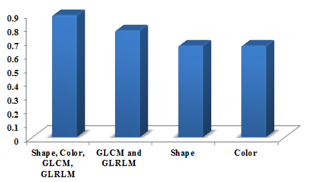
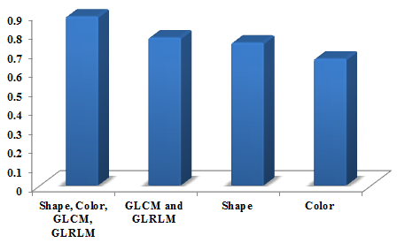
In Figure 1 the performance graph for sensitivity is shown as 0.88. The features vary based on a number of features such as shape, color, GLCM, and GLRLM. The number of these whole features is performed better compared with other less number of features namely GLCM and GLRLM, Shape, Color.
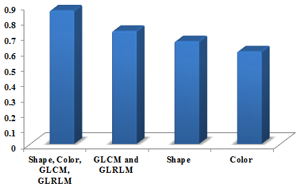
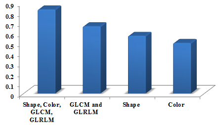
In Figure 2 the performance graph for specificity is shown as 0.83. The features vary based on the number of features such as shape, color, GLCM, and GLRLM. The number of these whole features is performed better compared with other less number of features namely GLCM and GLRLM, shape, color.
Figure 1. Performance graph for sensitivity
Figure 2. Performance graph for specificity
In Figure 3 the performance graph for accuracy is shown as 0.86. The features vary based on the number of features such as shape, color, GLCM, and GLRLM. The number of these whole features is performed better compared with other less number of features namely GLCM and GLRLM, Shape, Color.
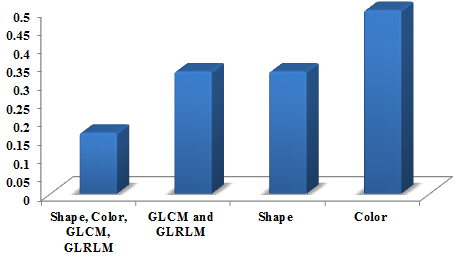
In Figure 4 the performance graph for FPR is shown as 0.16. The features vary based on the number of features such as shape, color, GLCM, and GLRLM. The number of these whole features is performed better compared with other less number of features namely GLCM and GLRLM, Shape, Color.
Figure 3. Performance graph for Accuracy
Figure 4. Performance graph for FPR
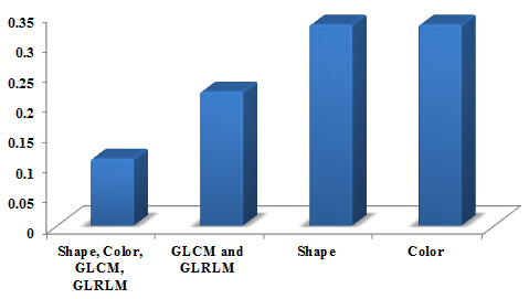
In Figure 5 the performance graph for FNR is shown as 0.11. The features vary based on the number of features such as shape, color, GLCM, and GLRLM. The number of these whole features is performed better compared with other less number of features namely GLCM and GLRLM, Shape, Color.
In Figure 6 the performance graph for PPV is shown as 0.88. The features vary based on the number of features such as shape, color, GLCM, and GLRLM. The number of these whole features is performed better compared with other less number of features namely GLCM and GLRLM, shape, color.
Figure 5. Performance graph for FNR
Figure 6. Performance graph for PPV
Figure 7. Performance graph for NPV
Figure 8. Performance graph for FDR
In Figure 7 the performance graph for NPV is shown as 0.83. The features vary based on the number of features such as shape, color, GLCM, and GLRLM. The number of these whole features is performed better compared with other less number of features namely GLCM and GLRLM, Shape, Color.
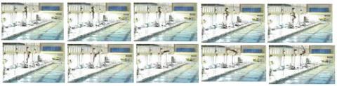
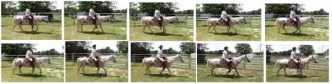
In Figure 8 the performance graph for FDR is shown as 0.11. The features vary based on the number of features such as shape, color, GLCM, and GLRLM. The number of these whole features is performed better compared with other less number of features namely GLCM and GLRLM, Shape, Color. Table 2 shows the video convert into different sample frames.
Table 2. Video convert into different sample frames
|
Video |
Sample frames |
|
1 |
|
|
2 |
|
|
3 |
|
|
4 |
|
|
5 |
This investigation concludes with the evident results of implementing feature extraction techniques for identifying duplication video. The performance yielded sensitivity value for shape, color, GLCM, and GLRLM as 0.88, specificity value for shape, color, GLCM, and GLRLM as 0.83 and accuracy value for shape, color, GLCM, and GLRLM as 0.86. A direction for future work is to raise the efficiency of our proposed scheme by exploring and combining additional features there by reducing the number of candidates selected in the coarse search.
[1] Lin, G.S., Chang, J.F. (2012). Detection of frame duplication forgery in videos based on spatial and temporal analysis. International Journal of Pattern Recognition and Artificial Intelligence, 26(7): 1-18. https://doi.org/10.1142/S0218001412500176
[2] Nie, Z.H., Hua, Y., Feng, D., Li, Q.Y., Sun, Y.Y. (2014). Efficient storage support for real-time near-duplicate video retrieval. International Conference on Algorithms and Architectures for Parallel Processing, pp. 312-324. https://doi.org/10.1007/978-3-319-11194-0_24
[3] Ulutas, G.Z., Ustubioglu, B., Ulutas, M., Nabiyev, V. (2017). Frame duplication/mirroring detection method with binary features. IET Image Processing, 11(5): 333-342. https://doi.org/10.1049/iet-ipr.2016.0321
[4] Liu, Y.Y., Zhu, C., Mao, M., Song, F.L., Dufaux, F., Zhang, X. (2017). Analytical distortion aware video coding for computer based video analysis. IEEE 19th International Workshop on Multimedia Signal Processing (MMSP), pp. 1-6. https://doi.org/10.1109/MMSP.2017.8122253
[5] Kordopatis-Zilos, G., Papadopoulos, S., Patras, I., Kompatsiaris, Y. (2017). Near-duplicate video retrieval with deep metric learning. IEEE Transaction, pp. 347-356. https://doi.org/10.1109/ICCVW.2017.49
[6] Verdoliva, L., Cozzolino, D., Poggi, G. (2014). A feature-based approach for image tampering detection and localization. IEEE International Workshop on Information Forensics and Security, pp. 149-154. https://doi.org/10.1109/WIFS.2014.7084319
[7] Li, C., Ma, Q., Xiao, L., Li, M., Zhang, A. (2017). Image splicing detection based on Markov features in QDCT domain. Neurocomputing, 228: 29-36. https://doi.org/10.4018/IJDCF.2018100107
[8] Zhao, X., Wang, S., Li, S., Li, J. (2015). Passive image-splicing detection by a 2-D noncausal Markov model. IEEE Transactions on Circuits and Systems for Video Technology, 25: 185-199. https://doi.org/10.1109/TCSVT.2014.2347513
[9] Manu, V.T., Mehtre, B.M. (2016). Detection of copy-move forgery in images using segmentation and surf. Springer International Publishing, Cham, pp. 645–654. https://doi.org/10.1007/978-3-319-28658-7_55
[10] Pun, C.-M., Liu, B., Yuan, X.-C. (2016). Multi-scale noise estimation for image splicing forgery detection. Journal of Visual Communication and Image Representation, 38: 195-206. https://doi.org/10.1016/j.jvcir.2016.03.005
[11] Ferreira, C.D., Santos, J.A., Torres, R. da S., Goncalves, M.A., Rezende, R.C., Fan, W.G. (2011). Relevance feedback based on genetic programming for image retrieval. Pattern Recognition Letters, 32(1): 27-37. https://doi.org/10.1016/j.patrec.2010.05.015
[12] Hu, G.H., Wang, Q.H., Zhang, G.H. (2015). Unsupervised defect detection in textiles based on Fourier analysis and wavelet shrinkage. Journal of Optical Society of America, 54(10): 2963-2980. https://doi.org/10.1364/AO.54.002963
[13] Bharathi, P.T., Subashini, P. (2013). Texture feature extraction of infrared river ice images using second-order spatial statistics. International Journal of Computer and Information Engineering, 7(2): 195-205. https://doi.org/10.5281/zenodo.1083681
[14] Karamti, H., Tmar, M., Gargouri, F. (2014). Content-based image retrieval system using neural networks. International Conference on Computer Systems and Applications (AICCSA), pp. 723-728. https://doi.org/10.1109/AICCSA.2014.7073271
[15] Lin, G.S., Chang, J.F., Chuang, C.H. (2011). Detecting frame duplication based on spatial and temporal analyses. International Conference on Computer Science & Education, pp. 1396-1399. https://doi.org/10.1109/ICCSE.2011.6028891
[16] Rana, S.P., Dey, M., Siarry, P. (2019). Boosting content-based image retrieval performance through the integration of parametric & nonparametric approaches. Journal of Visual Communication and Image Representation, 58: 205-219. https://doi.org/10.1016/j.jvcir.2018.11.015
[17] Taşci, T. (2018). Image mining: techniques for feature extraction. Intelligent Techniques for Data Analysis in Diverse Settings, pp. 66-95. https://doi.org/10.4018/978-1-5225-0075-9.ch004
[18] Nian, F.D., Li, T., Wang, Y., Wu, X.Y., Ni, B.B., Xu, C.S. (2017). Learning explicit video attributes from mid-level representation for video captioning. Computer Vision and Image Understanding, 163: 126-138. https://doi.org/10.1016/j.cviu.2017.06.012
[19] Yang, J.M., Huang, T.Q., Su, L.C. (2016). Using similarity analysis to detect frame duplication forgery in videos. Multimedia Tools and Applications, 75(4): 1793-1811. https://doi.org/10.1007/s11042-014-2374-7
[20] Singh, V.K., Tripathi, R.C. (2011). Fast and efficient region duplication detection in digital images using sub-blocking method. International Journal of Advanced Science and Technology, 35: 93-102. https://doi.org/10.1.1.359.7252