Benyettou Loutfi* | Zeghlache Samir | Djerioui Ali | Ghellab Mohammed Zinelaabidine
© 2019 IIETA. This article is published by IIETA and is licensed under the CC BY 4.0 license (http://creativecommons.org/licenses/by/4.0/).
OPEN ACCESS
The work has done in this paper concern a strategy of control based on real time implementation of backstepping sliding mode using the interval type-2 fuzzy logic and their application to the Twin Rotor MIMO System (TRMS), the backstepping sliding mode controller are the problem of the chattering phenomenon, this can damage the actuators and disrupt the operation and performance of the system, so to reduce this problem we combine the fuzzy logic type 2. The proposed techniques were applied to the TRMS, where the real time implementation of type-2 fuzzy backstepping sliding mode controller (T2FBSMC) were proposed for control system in the presence of external distrubances. The interval type-2 fuzzy logic is used to minimize the major problem of sliding mode and employed in the stability analysis. The obtained simulation and experiment results confirm the effectiveness of the proposed method.
TRMS model, interval type-2 fuzzy logic, sliding mode, backstepping, T2FBSMC
The autopilot of planes and helicopters was born with modern aviation and has evolved over time to meet increasingly restrictive needs. It can be used when the task to be performed is too repetitive or too difficult for the pilot. The control of the automatic control of the evolution of helicopters controlled by radio opens the way to applications in the fields of security (surveillance of the airspace, the urban and interurban traffic), the management of the natural risks (monitoring of volcano activity), the environment (measurement of air pollution, forest monitoring), for intervention in hostile environments (radioactive environments, demining of land without human intervention), management major infrastructures (dams, high-voltage lines, pipelines), agriculture (detection and treatment of infested crops) and aerial photography in film production [1, 2].
The TRMS (Twin Rotor MIMO System) is an aerodynamic physical system similar to a helicopter, designed for the development and implementation of new control laws. [3- 5] Several works have been done to control of the TRMS, the researchers have been developed the control strategies to solve the problems of this type of system. The sliding mode control, is a robust control in the presence of parametric variations, characterized by its robustness against nonlinearity and its efficiency in the rejection of disturbances, [6, 7], in [8] sliding mode control is designed for a linearized model of the TRMS system. The authors in [9], proposed an adaptive second-order sliding mode controller in objectives to stabilize and control the TRMS system in significant cross couplings, in [10], a model for the TRMS is used based an optimal linear quadratic regulator and a sliding mode controller. Real-time control of the vertical and horizontal positions of TRMS using a decentralized sliding mode controller is presented in [11].
The major disadvantage of sliding mode is the chattering phenomenon, which can damage the actuators by too frequent stress and impair the operation and performance of the system, in order to reduce these oscillations several solutions have been made, for example: use artificial intelligence tools, including fuzzy logic type 1 and type 2, in [2] authors presented the real time implementation of non linear observer-based on type-1 fuzzy sliding mode controller for TRMS system, the proposed control in this paper can be attenuating the chattering phenomena of the sliding mode control. In [12, 13] the type 2 fuzzy logic and adaptive type 2 fuzzy logic controllers are proposed to stabilize the TRMS Helicopter system, using two independent type-2 fuzzy controllers for the yaw and pitch angles of the TRMS, the performance of each control scheme is examined under a number of simulations.
In this work, the real time implementation of T2FBSMC approaches for a TRMS system is proposed. An interval type-2 fuzzy logic is used to solve the chattering problem due to the correction term. Compared to previous studies on sliding mode control [9, 11], the proposed control approach can reduce the chattering phenomenon and obtained a good dynamic response. Compared to boundary layer sliding mode control [2, 10] and higher order sliding mode control, the control approach can also reduce these oscillations. The contributions of this paper could be briefly summarized as follows.
The rest of the paper is organized as follows. Section 2 focuses on the nonlinear dynamic model of the 2-DOF helicopter (TRMS). Design of the T2FBSMC is highlighted in section 3 and 4. Simulation results and related discussions are given in section 5. The experimental results to validate the effectiveness of the proposed approach are presented in Section 6. Finally some conclusions are drawn in section 7.
Similar to most flight vehicles, the helicopter consists of several elastic parts such as rotor, engine and control surfaces. The nonlinear aerodynamic forces and gravity act on the vehicle, and flexible structures increase complexity and make a realistic analysis difficult. For control purpose, it is necessary to find a representative model that shows the same dynamic characteristics as the real aircraft [14]. The behaviour of a nonlinear TRMS, (shown in Figure 1), in certain aspects resembles that of a helicopter. It can be well perceived as a static test rig for an air vehicle with formidable control challenges.
Figure 1. The twin rotor multi-input multi-output system (TRMS) [15]
This TRMS consists of a beam pivoted on its base in such a way that it can rotate freely in both its horizontal and vertical planes. There are two rotors (the main and tail rotors), driven by DC motors, at each end of the beam. If necessary, either or both axes of rotation can be locked by means of two locking screws provided for physically restricting the horizontal or vertical plane rotation. Thus, the system permits both 1 and 2 degree-of-freedom (DOF) experiments. The two rotors are controlled by variable speed electric motors enabling the helicopter to rotate in a vertical and horizontal plane (pitch and yaw). The tail rotor could be rotated in either direction, allowing the helicopter to yaw right or left. The motion of the helicopter was damped by a pendulum, which hung from a central pivot point. In a typical helicopter, the aerodynamic force is controlled by changing the angle of attack of the blades. The laboratory setup is constructed such that the angle of attack of the blades is fixed. The aerodynamic force is controlled by varying the speed of the motors. The mathematical model of the TRMS is developed under following assumptions.
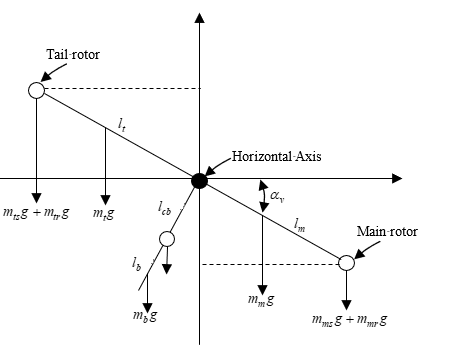
The mechanical system of TRMS is simplified using a four point-mass system shown in Figure 2, includes main rotor, tail rotor, balance-weight and counter-weight. Based on Lagrange’s equations, we can classify the mechanical system into two parts, the forces around the horizontal axis and the forces around the vertical axis.
Figure 2. Simplified four point-mass system
The parameters in the simplified four point-mass system are Mv1 is the return torque corresponding to the force of gravity, Mv2 is the moment of a centrifugal forces, Mv3 is a Moment of friction, Mv4 is the mass of the DC motor within the main rotor, mmr is the mass of the main part of the beam, mm is the mass of the DC motor within tail rotor, mtr is the mass of the tail part of the beam, mt is the mass of the counter weight, mcb is the mass of the tail shield, mb is the length of the main part of the beam, mms is the length of the tail part of the beam, lm is the length of the counter-weight beam, lt is the distance between the counter-weight and joint, and g is the gravitational acceleration. Consider the rotation of the beam in the vertical plane (around the horizontal axis). The driving torqueses are produced by the propellers, and the rotation can be described in principle as the motion of a pendulum. We can write the equations describing this motion as follows:
2.1 The main rotor model
${{M}_{v1}}=g\left\{ \left[ \left( \frac{{{m}_{t}}}{2}+{{m}_{tr}}+{{m}_{ts}} \right)\ {{l}_{t}}-\left( \frac{{{m}_{m}}}{2}+{{m}_{mr}}+{{m}_{ms}} \right)\ {{l}_{m}} \right]\cos \ {{\alpha }_{v}}-\left( \frac{{{m}_{b}}}{2}{{l}_{b}}+{{m}_{cb}}\ \ {{l}_{cb}} \right)\sin {{\alpha }_{v}} \right\}$ (1)
${{M}_{v1}}=g\ \left\{ \left[ A-B \right]\cos \ {{\alpha }_{v}}-C\sin \ {{\alpha }_{v}} \right\}$ (2)
with:
$\left\{ \begin{align} & A=\left( \frac{{{m}_{t}}}{2}+{{m}_{tr}}+{{m}_{ts}} \right){{l}_{t}} \\ & B=\left( \frac{{{m}_{m}}}{2}+{{m}_{mr}}+{{m}_{ms}} \right)\ {{l}_{m}} \\ & C=\left( \frac{{{m}_{b}}}{2}{{l}_{b}}+{{m}_{cb}}\ \ {{l}_{cb}} \right) \\ \end{align} \right.$ (3)
${{M}_{v2}}={{l}_{m}}{{S}_{f}}{{F}_{v}}\left( {{\omega }_{m}} \right)$ (4)
The angular velocity ωm of main propeller is a nonlinear function of a rotation angle of the DC motor describing by:
${{\omega }_{m}}\left( {{u}_{vv}} \right)=90.90\ u_{vv}^{6}+599.73\ u_{vv}^{5}-129.26\ u_{vv}^{4}-1238.64\ u_{vv}^{3}\ +63.45\ u_{vv}^{2}+1238.41\ u_{vv}^{{}}$(5)
Also, the propulsive force Fv moving the joined beam in the vertical direction is describing by a nonlinear function of the angular velocity ωm
${{F}_{v}}\left( {{\omega }_{m}} \right)=-3.48\times {{10}^{-12}}\omega _{m}^{5}+1.09\times {{10}^{-9}}\omega _{m}^{4}+4.123\times {{10}^{-6}}\omega _{m}^{3}-1.632\times {{10}^{-4}}\omega _{m}^{2}+9.544\times {{10}^{-2}}{{\omega }_{m}}$ (6)
The model of the motor-propeller dynamics is obtained by substituting the nonlinear system by a serial connection of a linear dynamics system. This can be expressed as:
$\frac{d{{u}_{vv}}}{dt}=\frac{1}{{{T}_{mr}}}\left( -{{u}_{vv}}+{{u}_{v}} \right)$ (7)
uv is the input voltage of the DC motor, Tmr is the time constant of the main rotor and Kmr is the static gain DC motor.
Figure 3. The relationship between the input voltage and the propulsive force for the main rotor
${{M}_{v3}}=-\Omega \ _{h}^{2}\ \left\{ \left( \frac{{{m}_{t}}}{4}+{{m}_{tr}}+{{m}_{ts}} \right)l_{t}^{2}+\left( \frac{{{m}_{t}}}{4}+m{{\ }_{tr}}+{{m}_{ts}} \right)l_{m}^{2}-\left( \frac{{{m}_{b}}}{4}l_{b}^{2}+{{m}_{cb}}\ l_{cb}^{2} \right) \right\}\ \sin \ \ {{\alpha }_{v}}\cos \ \ {{\alpha }_{v}}$ (8)
${{M}_{v3}}=-\Omega \ _{h}^{2}\ \left( H \right)\sin \ \ {{\alpha }_{v}}\cos \ \ {{\alpha }_{v}}$ (9)
with:
$H=\left( \frac{{{m}_{t}}}{4}+m{{\ }_{tr}}+m{{\ }_{ts}} \right)\ l_{t}^{2}+\left( \frac{{{m}_{t}}}{4}+m{{\ }_{tr}}+m{{\ }_{ts}} \right)\ l_{m}^{2}-\left( \frac{{{m}_{b}}}{4}l_{b}^{2}\ +\ \ {{m}_{cb}}\ l_{cb}^{2} \right)$ (10)
${{\Omega }_{h}}=\frac{d{{\alpha }_{h}}}{dt}$ (11)
${{M}_{v4}}=-{{\Omega }_{v}}{{K}_{v}}$ (12)
${{\Omega }_{v}}=\frac{d{{\alpha }_{v}}}{dt}$ (13)
$\frac{d{{S}_{v}}}{dt}=\frac{1}{{{J}_{v}}}\sum\limits_{i=1}^{4}{{{M}_{vi}}}$ (14)
$\frac{dS{{\ }_{v}}}{dt}=\frac{1}{{{J}_{v}}}\left\{ {{l}_{m}}\ {{S}_{f}}\,{{F}_{v}}\ \left( {{\omega }_{m}} \right)-{{K}_{v}}\ {{\Omega }_{v}}+g\ \left( \left( A-B \right)\cos \ \ \ {{\alpha }_{v}}-C\ \sin \ \ \ {{\alpha }_{v}} \right)\ -\Omega _{h}^{2}\,\left( H \right)\sin \ {{\alpha }_{v}}\ \cos \ {{\alpha }_{v}} \right\}$ (15)
$\frac{d{{\alpha }_{v}}}{dt}={{\Omega }_{v}}={{S}_{v}}+\frac{{{J}_{tr}}{{\omega }_{t}}}{{{J}_{v}}}$ (16)
where $ω_t$ is the angular velocity of tail propeller, Sv the angular momentum in the vertical plane of the beam, Jv the sum of inertia moments in the horizontal plane, Jtr the moment of inertia in DC motor tail propeller subsystem, Kv the Friction constant, and Sf the balance scale.
2.2 The tail rotor model
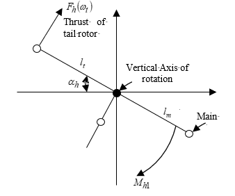
Similarly, we can describe the motion of the beam in the horizontal plane (around the vertical axis) as shown in Figure .4. The driving torques’s are produces by the rotors and that the moment of inertia depends on the pitch angle of the beam.
Figure 4. Torques around the vertical axis
The parameters in the torques around vertical axis are Mh1 is the moment of an aerodynamic force, Mh2 is a Moment of friction.
${{M}_{h1}}={{l}_{t}}{{S}_{f}}{{F}_{h}}\left( {{\omega }_{t}} \right)\ \cos {{\alpha }_{v}}$ (17)
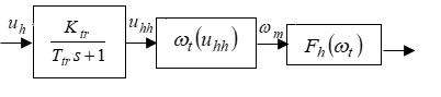
The angular velocity ωt of tail is a nonlinear function describing by:
${{\omega }_{t}}\left( {{u}_{hh}} \right)=2020\ u_{hh}^{5}+194.69\ u_{hh}^{4}-4283.15\ u_{vv}^{3}-262.87\ u_{hh}^{2}\ +3796.83\ u_{hh}^{{}}$ (18)
Also, the propulsive force Fh moving the joined beam in the Horizontal direction is describing by
${{F}_{h}}\left( {{\omega }_{t}} \right)=-3\times {{10}^{-14}}\omega _{t}^{5}+1.595\times {{10}^{-11}}\omega _{t}^{4}+2.511\times {{10}^{-7}}\omega _{t}^{3}-1.808\times {{10}^{-4}}\omega _{t}^{2}+0.8080\ \ {{\omega }_{t}}$ (19)
The model of the motor-propeller dynamics is obtained by substituting the nonlinear system by a serial connection of a linear dynamics system. This can be expressed as:
$\frac{d{{u}_{hh}}}{dt}=\frac{1}{{{T}_{tr}}}\left( -{{u}_{hh}}+{{u}_{h}} \right)$ (20)
uh is the input voltage of the DC motor, Ttr is the time constant of the tail rotor and Ktr is the static gain DC motor.
Figure 5. The relationship between the input voltage and the propulsive force for the tail rotor
${{M}_{h2}}=-{{\Omega }_{h}}{{K}_{h}}$ (21)
$\frac{d{{S}_{h}}}{dt}=\frac{1}{{{J}_{h}}\left( {{\alpha }_{v}} \right)}\sum\limits_{i=1}^{4}{{{M}_{hi}}}$ (22)
${{J}_{h}}\left( {{\alpha }_{v}} \right)=D\ {{\cos }^{2}}{{\alpha }_{v}}+E\ {{\sin }^{2}}{{\alpha }_{v}}+F\frac{d{{S}_{h}}}{dt}=\frac{{{l}_{t}}{{S}_{f}}{{F}_{h}}\left( {{\omega }_{t}} \right)\cos \ \alpha {}_{v}-{{\Omega }_{h}}{{K}_{h}}}{{{J}_{h}}\left( {{\alpha }_{v}} \right)}$ (23)
$\frac{d{{S}_{h}}}{dt}=\frac{{{l}_{t}}{{S}_{f}}{{F}_{h}}\left( {{\omega }_{t}} \right)\cos \ \alpha {}_{v}-{{\Omega }_{h}}{{K}_{h}}}{D\ {{\cos }^{2}}{{\alpha }_{v}}+E\ {{\sin }^{2}}{{\alpha }_{v}}+F}$ (24)
$\frac{d{{\alpha }_{h}}}{dt}={{\Omega }_{h}}={{S}_{h}}+\frac{{{J}_{mr}}\ {{\omega }_{m}}\ \cos \ {{\alpha }_{v}}}{D\ {{\cos }^{2}}{{\alpha }_{v}}+E\ {{\sin }^{2}}{{\alpha }_{v}}+F}$ (25)
where, Sh the angular momentum in the horizontal plane of the beam, Jh the sum of inertia moments in the vertical plane, Jmr the moment of inertia in DC motor main propeller subsystem, Kh the Friction constant, and Sf the balance scale.
The dynamics of the TRMS system are described as follows:
$\left\{ \begin{align}& \frac{dS{{\ }_{v}}}{dt}=\frac{1}{{{J}_{v}}}\left\{ {{l}_{m}}\ {{S}_{f}}\,{{F}_{v}}\ \left( {{\omega }_{m}} \right)-{{K}_{v}}\ {{\Omega }_{v}}+g\ \left( \left( A-B \right)\cos \ {{\alpha }_{v}}-C\ \sin \ {{\alpha }_{v}} \right)\ -\Omega _{h}^{2}\,\left( H \right)\sin \ {{\alpha }_{v}}\ \cos \ {{\alpha }_{v}} \right\} \\ & {{\Omega }_{v}}=\frac{d{{\alpha }_{v}}}{dt} \\ & {{\Omega }_{v}}={{S}_{v}}+\frac{{{J}_{tr}}{{\omega }_{t}}}{{{J}_{v}}} \\ & \frac{d{{S}_{h}}}{dt}=\frac{{{l}_{t}}\ {{S}_{f}}\ {{F}_{h}}\ \left( {{\omega }_{t}} \right)\cos \ \ \alpha {}_{v}-{{\Omega }_{h}}\ {{K}_{h}}}{{{J}_{h}}\left( {{\alpha }_{v}} \right)} \\ & {{\Omega }_{h}}=\frac{d{{\alpha }_{h}}}{dt} \\ & {{\Omega }_{h}}={{S}_{h}}+\frac{{{J}_{mr}}\ {{\omega }_{m}}\ \cos \ {{\alpha }_{v}}}{D\ {{\cos }^{2}}{{\alpha }_{v}}+E\ {{\sin }^{2}}{{\alpha }_{v}}+F} \\ \end{align} \right.$ (26)
The model developed in (26) can be rewritten in the state-space form:
$X ̇$=f(x)+g(X,U) and $X=[x_1,...,x_6 ]^T$ is the state vector of the system such as:
$X=[{{\alpha }_{v}},{{S}_{v}},{{u}_{vv}},{{\alpha }_{h}},{{S}_{h}},{{u}_{hh}}]$ (27)
$U=\left[ {{u}_{v}},{{u}_{h}} \right]$ (28)
$Y=\left[ {{\alpha }_{v}},{{\alpha }_{h}} \right]$ (29)
From (26), (28) and (29) we obtain the following state representation:
$\left\{ \begin{align} & {{{\dot{x}}}_{1}}\ =\ \ {{x}_{2}}+\ \ \frac{{{J}_{tr}}}{{{J}_{v}}}{{\omega }_{t}}\ \left( {{x}_{6}} \right) \\ & {{{\dot{x}}}_{2}}=\ \ \frac{1}{{{J}_{v}}}\,\left\{ {{l}_{m}}\ {{S}_{f}}\ {{F}_{v}}\ \left( {{\omega }_{m}}\ \left( {{x}_{3}} \right) \right)-{{K}_{v}}\left( {{x}_{2}}+\frac{{{J}_{tr}}}{{{J}_{v}}}{{\omega }_{t}}\ \left( {{x}_{6}} \right) \right)\ +g\ \left( \left( A\ \ -\ B\ \right)\cos \ x{{}_{1}}-\ \ C\ \sin \ {{x}_{1}} \right) \right.- \\ & \quad \quad \left. \ \,{{\left( {{x}_{5}}+\ \frac{{{J}_{mr}}\ {{\omega }_{m}}\left( {{x}_{3}} \right)\ \cos \ \ \ {{x}_{1}}}{D\ \ {{\cos }^{2}}{{x}_{\ 1}}+E\ {{\sin }^{2}}\ {{x}_{1}}+F} \right)}^{2}}\ \left( H \right)\sin \ {{x}_{1}}\ \cos \ {{x}_{1}} \right\} \\ & {{{\dot{x}}}_{3}}=\ \ \frac{1}{{{T}_{mr}}}\left( -{{x}_{3}}+{{K}_{mr}}\ {{u}_{v}} \right) \\ & {{{\dot{x}}}_{4}}=\ \ {{x}_{5}}+\ \frac{{{J}_{mr}}\ {{\omega }_{m}}\ \left( {{x}_{3}} \right)\ \cos \ {{x}_{1}}}{D\ \ {{\cos }^{2}}{{x}_{1}}+E\ \ {{\sin }^{2}}{{x}_{1}}+F} \\ & {{{\dot{x}}}_{5}}=\ \ \frac{1}{D\ \ {{\cos }^{2}}x{{\ }_{1}}+E\ {{\sin }^{2}}\ x{{\ }_{1}}+F}\ \left\{ {{l}_{t}}\ {{S}_{f}}\ {{F}_{h}}\ \left( {{\omega }_{t}} \right)\cos \ \alpha {}_{v}- \right. \\ & \quad \quad \left. {{K}_{h}}\ \left( {{x}_{5}}+\frac{{{J}_{mr}}\ {{\omega }_{m}}\left( {{x}_{3}} \right)\ \cos \ x{{\ }_{1}}}{D\ \ {{\cos }^{2}}x{{\ }_{1}}+E\ {{\sin }^{2}}\ {{x}_{1}}+F} \right) \right\} \\ & {{{\dot{x}}}_{6}}=\ \ \frac{1}{{{T}_{tr}}}\left( -{{x}_{6}}+{{K}_{tr}}\ {{u}_{h}} \right) \\ \end{align} \right.$ (30)
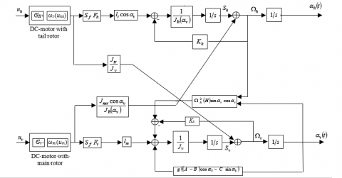
Figure 2 shows the block diagram of the TRMS helicopter, where is characterized by cross-coupling, complex dynamics.
Figure 6. Block diagram of TRMS system
Since the characteristic of TRMS is very complex in the nature, it would be convenient to design a controller for TRMS with the TRMS decoupled into horizontal and vertical subsystems by fixing the horizontal angle ah and posing uh=0 , from Eq. (30), it is easy to see that state equations with the state vector Xv for the vertical subsystem of the TRMS could be defined as:
${{X}_{v}}=\left[ {{x}_{1}},{{x}_{2}},{{x}_{3}} \right]=\left[ {{\alpha }_{v}},{{S}_{v}},{{u}_{vv}} \right]$ (31)
$\left\{ \begin{align} & {{{\dot{x}}}_{1}}\ =\ \ {{x}_{2}} \\ & {{{\dot{x}}}_{2}}=\ \ \frac{1}{{{J}_{v}}}\left\{ {{l}_{m}}\ {{S}_{f}}\ {{F}_{v}}\ \left( {{\omega }_{m}}\ \left( {{x}_{3}} \right) \right)-{{K}_{v}}\left( {{x}_{2}} \right)\ +g\ \left( \left( A\ -\ B\ \right)\ \cos \ \ x{{\ }_{1}}-\ \ C\ \sin \ {{x}_{1}} \right) \right\} \\ & {{{\dot{x}}}_{3}}=\ \ \frac{1}{{{T}_{mr}}}\left( -{{x}_{3}}+{{K}_{mr}}\ {{u}_{v}} \right) \\ \end{align} \right.$ (32)
where, uv is a control action of the vertical subsystem Likewise, we have the horizontal subsystem by posing $α_v=α_v (0)=α_v0$ and $u_v =(0)$
${{X}_{h}}=\left[ {{x}_{4}},{{x}_{5}},{{x}_{6}} \right]=\left[ {{\alpha }_{h}},{{S}_{h}},{{u}_{hh}} \right]$ (33)
$\left\{ \begin{align} & {{{\dot{x}}}_{4}}=\ \ {{x}_{5}} \\ & {{{\dot{x}}}_{5}}=\ \ \frac{1}{{{J}_{h}}\left( {{\alpha }_{v0}} \right)}\ \left\{ {{l}_{t}}\ {{S}_{f}}\ {{F}_{h}}\ \left( {{\omega }_{t}} \right)\cos \ \alpha {}_{v0}-\ {{K}_{h}}\ {{x}_{5}} \right\} \\ & {{{\dot{x}}}_{6}}=\ \ \frac{1}{{{T}_{tr}}}\left( -{{x}_{6}}+{{K}_{tr}}\ {{u}_{h}} \right) \\ \end{align} \right.$ (34)
The parameters of the model are shown in Table 1.
Table 1. The parameters of the TRMS [15]
|
Symbol |
Definition |
Value |
|
A |
Mechanical related constant |
0.0946875 kgm2 |
|
B |
Mechanical related constant |
0.11046 kgm2 |
|
C |
Mechanical related constant |
0.01986 kgm2 |
|
D |
Mechanical related constant |
0.04988 kgm2 |
|
E |
Mechanical related constant |
0.004745 kgm2 |
|
F |
Mechanical related constant |
0.006230 kgm2 |
|
H |
Mechanical related constant |
0.048210 kgm2 |
|
Sf |
Balanced scale |
0.000843318 |
|
Jv |
Sum of inertia moments in the horizontal plane |
0.055448 kgm2 |
|
Jmr |
Moment of inertia in the DC-motor of main propeller |
0.000016543 kgm2 |
|
Jtr |
Moment of inertia in the DC-motor of main propeller |
0.0000265 kgm2 |
|
lm |
Length of the main part of the beam |
0.24 m |
|
lt |
Length of the tail part of the beam |
0.25 m |
|
Tmr |
Time constant of the main rotor |
1.432 sec |
|
Ttr |
Time constant of the tail rotor |
0.3842 sec |
|
Kmr |
Static gain of the main DC-motor |
1 |
|
Ktr |
Static gain of the tail DC-motor |
1 |
|
Kv |
Friction coefficient for the vertical axis |
0.0095 |
|
Kh |
Friction coefficient for the horizntal axis |
0.00545371 |
|
g |
Gravitational acceleration |
9.81 m/s2 |
Type-1 and type-2 fuzzy logic are mainly similar. However, there exist two essential differences between them which are: the membership functions shape and the output processor. Indeed, an interval type-2 fuzzy controller is consisting of: a fuzzifier, an inference engine, a rules base, a type reduction and a defuzzyfier.
4.1 Fuzzifier
The fuzzifier maps the crisp input vector $(e_1,e_2,…,e_n )^T$ to a type-2 fuzzy system $A ̃_x$, very similar to the procedure performed in a type-1 fuzzy logic system.
4.2 Rules
The general form of the ith rule of the type-2 fuzzy logic system can be written as:
If $e_1$ is $F ̃_1^i$ and $e_2$ is $F ̃_2^i$ and … $e_n$ is $F ̃_n^i$, Than
$y^i=G ̃^i i=1,…,M$ (35)
where, $F ̃_j^i$ represents the type-2 fuzzy system of the input state j of the ith rule, $x_1$, $x_2$, …,$x_n$ are the inputs, $G ̃^i$ is the output of type-2 fuzzy system for the rule i, and M is the number of rules. As can be seen, the rule structure of type-2 fuzzy logic system is similar to type-1 fuzzy logic system except that type-1 membership functions are replaced with their type-2 counterparts.
4.3 Inference Engine
In fuzzy system interval type-2 using the minimum or product t-norms operations, the ith activated rule $F^i (x_1,…x_n)$ gives us the interval that is determined by two extremes $▁f^i (x_1,…x_n)$ and $¯f^i (x_1,…x_n)$ [16]:
${{F}^{i}}\left( {{x}_{1}},\ldots {{x}_{n}} \right)=[{{\underline{\ f}}^{i}}({{x}_{1}},\ldots {{x}_{n}}),{{\overline{f}}^{i}}({{x}_{1}},\ldots {{x}_{n}})]\equiv [{{\underline{f}}^{i}},{{\overline{f}}^{i}}]$ (36)
with $▁f^i$ and $¯f^i$ are given by:
$\begin{align} & {{\underline{f}}^{i}}={{\underline{\mu }}_{F_{1}^{i}}}\left( {{x}_{1}} \right)*\ldots *{{\underline{\mu }}_{F_{n}^{i}}}\left( {{x}_{n}} \right) \\ & \\ & {{\overline{f}}^{i}}={{{\bar{\mu }}}_{F_{1}^{i}}}\left( {{x}_{1}} \right)*\ldots *{{{\bar{\mu }}}_{F_{n}^{i}}}\left( {{x}_{n}} \right) \\ \end{align}$ (37)
4.4 Type reducer
After the rules are fired and the inference is executed, the obtained type-2 fuzzy system resulting in a type-1 fuzzy system is computed. In this part, the available methods to compute the centroid of type-2 fuzzy system using the extension principle [17] are discussed. The centroid of type-1 fuzzy system A is given by:
${{C}_{A}}=\frac{\sum\limits_{i=1}^{n}{{{z}_{i}}{{w}_{i}}}}{\sum\limits_{i=1}^{n}{{{w}_{i}}}}$ (38)
where, n represents the number of discretized domain of A, $z_i∈R$ and $w_i∈[0, 1]$.
If each $z_i$ and $w_i$ are replaced, using the extension principle, with a type-1 fuzzy system, $Z_i$ and $W_i$, the generalized centroid for type-2 fuzzy system $\overset{-}{\mathop{\text{A}}}\,$ is given by:
$G{{C}_{{\tilde{A}}}}=\int\limits_{{{z}_{1}}\in {{Z}_{1}}}{\ldots \int\limits_{{{z}_{n}}\in {{Z}_{n}}}{\int\limits_{{{w}_{1}}\in {{W}_{1}}}{\ldots \int\limits_{{{w}_{n}}\in {{W}_{n}}}{\left[ T_{i=1}^{n}{{\mu }_{Z}}\left( {{z}_{i}} \right)*T_{i=1}^{n}{{\mu }_{W}}\left( {{z}_{i}} \right) \right]/\frac{\sum\limits_{i=1}^{n}{{{z}_{i}}{{w}_{i}}}}{\sum\limits_{i=1}^{n}{{{w}_{i}}}}}}}}$ (39)
where, $μ_Z (z_i)$ and $μ_W(W_i)$are the associated membership functions. T is a t-norm and $GC_A ̃$ is a type-1 fuzzy system.
For an interval type-2 fuzzy system:
$G{{C}_{{\tilde{A}}}}=\left[ {{y}_{l}}\left( x \right),{{y}_{r}}\left( x \right) \right]$
$=\int_{{{y}^{_{1}}}\in \left[ y_{l}^{1},y_{r}^{1} \right]}{\ldots \int_{{{y}^{_{M}}}\in \left[ y_{l}^{M},y_{r}^{M} \right]}{\ldots \int_{{{f}^{_{1}}}\in \left[ {{\underline{f}}^{1}},{{\overline{f}}^{1}} \right]}{\ldots }}}\int_{{{f}^{M}}\in \left[ {{\underline{f}}^{M}},\overline{f}_{{}}^{M} \right]}{1/\frac{\sum\limits_{i=1}^{M}{{{f}^{_{i}}}\ {{y}^{_{i}}}}}{\sum\limits_{i=1}^{M}{{{f}^{i}}}}}$ (40)
4.5 Deffuzzifier
To get a crisp output from a type-1 fuzzy logic system, the type-reduced set must be defuzzied. The most common method to do this is to find the centroid of the type-reduced set. If the type-reduced set Y is discretized to n points, then the following expression gives the centroid of the type-reduced set as:
${{y}_{output}}\left( x \right)=\frac{\sum\limits_{i=1}^{n}{{{y}^{i}}\mu \left( {{y}^{i}} \right)}}{\sum\limits_{i=1}^{m}{\mu \left( {{y}^{i}} \right)}}$ (41)
The output has been computed using the iterative Karnik Mendel algorithms [18-22]. Therefore, the defuzzified output of an interval type-2 FLC is:
${{Y}_{output}}\left( x \right)=\frac{{{y}_{l}}\left( x \right)+{{y}_{r}}\left( x \right)}{2}$ (42)
with: ${{y}_{l}}\left( x \right)=\frac{\sum\limits_{i=1}^{M}{f_{l}^{i}y_{l}^{i}}}{\sum\limits_{i=1}^{M}{f_{l}^{i}}}$ and
${{y}_{r}}\left( x \right)=\frac{\sum\limits_{i=1}^{M}{f_{r}^{i}y_{l}^{i}}}{\sum\limits_{i=1}^{M}{f_{r}^{i}}}$ (43)
The advantage of control algorithms based on sliding mode techniques is its insensitivity to the model errors and parametric uncertainties, as well as the ability to globally stabilize the system in the presence of other disturbances.
The recursive nature of the proposed control design is similar to the standard backstepping methodology. However, the proposed control design uses backstepping to design virtual controllers with a zero-order sliding surface at each recursive step. The benefit of this approach is that each virtual controller can compensate for unknown bounded function which contains unmodelled dynamics and external disturbances [23].
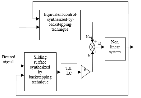
The control algorithms based on sliding mode techniques suffers from a main disadvantage that is chattering effect, which is the high frequency oscillation of the controller output. To overcome this problem and in order to reduce the chattering phenomenon, an interval type-2 fuzzy system is used to approximate the hitting control term. The configuration of the proposed type-2 fuzzy backstepping sliding mode control (T2FBSMC) scheme is shown in Figure 7; it contains an equivalent control part and single input single output interval type-2 fuzzy logic.
Figure 7. Block diagram of the IT2FSMC
The equivalent control $u_eq$, is calculated in such a way as to have $\overset{.}{\mathop{\text{s}}}\,$. Then the hitting control is computed by:
${{u}_{r}}={{k}_{fs}}{{u}_{fs}}$ (44)
${{u}_{fs}}=T2FLC\ \left( s \right)$ (45)
where, $(k_{fs}>0)$ is the normalization factor of the output variable, and $u_{fs}$ is the output of the T2FLC, which is obtained by the normalized s.
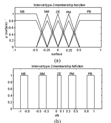
The fuzzy type-2 membership functions of the input sliding surface(s), and the output discontinuous control ($u_{fs}$) sets are presented by Figure 8.
In order to attenuate the chattering effect and handle the uncertainty of the six rotors helicopter, a type‐2 fuzzy controller has been used with single input and single output for each subsystem. Then, the input of the controller is the sliding surface and the output is the discontinuous control $u_{fs}$. All the membership functions of the fuzzy input variable are chosen to be triangular and trapezoidal for all upper and lower membership functions. The used labels of the fuzzy variable (surface) are: {negative medium (NM), negative big (NB), zero (ZE), positive medium (NM), positive big (PB)}.
The corrective control is decomposed into five levels represented by a set of linguistic variables: negative big (NB), negative medium (NM), zero (ZE), positive medium (PM) and positive big (PB). Table.2 presents the rules base which contains five rules.
The membership functions of the input (sliding surface) and output (ufs) has been normalized in the interval [-1, 1], therefore: |{u_fs}|≤1.
Figure 8. Membership functions of input s and output ufs [24]
Table 2. Fuzzy rules for type-2 FLCs [24]
|
|
Rule 1 |
Rule 2 |
Rule 3 |
Rule 4 |
Rule 5 |
|
Surface |
PB |
PM |
ZE |
NM |
NB |
|
ufs |
NB |
NM |
ZE |
PM |
PB |
$u_{fs}$ given in equation (30) satisfies the following condition:
$s{{u}_{fs}}=-{{K}^{+}}\left| s \right|$(46)
where , K+>0 is positive constant determined by a fuzzy type-2 inference system.
Proof
The hitting control laws are computed by type-2 fuzzy logic inference using equations (42) and (43) and the iterative Karnik Mendel Algorithms presented in [16-22]. Where $α_i=[α_{ilow},α_{iup}]$ for i=[1,...,5] are the membership interval of rules 1 to 5 presented in Table 2. Moreover, $u_{fs} can be further analyzed as the following six conditions given thereafter. Only one of six conditions will occur for any value of the sliding surface according to Figure 3 [24].
Condition 1
Only rule 1 is activated ($s>0.5,\ \alpha {{}_{1}}=\left[ 0.8,1 \right],{{\alpha }_{j}}=\left[ 0,0 \right]$ for $j=2,3,4,5$)
$u_fs=T2FLC (s)=(-0.8-1)/2=-0.9$ (47)
Condition 2
Rule 1 and 2 are activated ($0.25<s<0.5,\ \alpha {{}_{1}}=\left[ {{\alpha }_{1low}},{{\alpha }_{1up}} \right],\ \alpha {{}_{2}}=\left[ {{\alpha }_{2low}},{{\alpha }_{2up}} \right],{{\alpha }_{j}}=\left[ 0,0 \right]$ for $j=3,4,5$)
and
${{u}_{fs}}=T2FLC\ \left( s \right)=\frac{1}{2}\left( \frac{-0.8\ {{\alpha }_{1low}}-0.3{{\alpha }_{2up}}}{{{\alpha }_{1low}}+{{\alpha }_{2up}}}+\frac{-\ {{\alpha }_{1up}}-0.5{{\alpha }_{2low}}}{{{\alpha }_{1up}}+{{\alpha }_{2low}}} \right)$ (48)
Condition 3
Rule 2 and 3 are activated ($0<s<0.25,\ \alpha {{}_{2}}=\left[ {{\alpha }_{2low}},{{\alpha }_{2up}} \right],\ \alpha {{}_{3}}=\left[ {{\alpha }_{3low}},{{\alpha }_{3up}} \right],{{\alpha }_{j}}=\left[ 0,0 \right]$ for $j=1,4,5$)
$0\le {{\alpha }_{2low}},{{\alpha }_{3low}}\le 0.8$ and $0\le \alpha {{}_{2up}},{{\alpha }_{3up}}\le 1$
${{u}_{fs}}=T2FLC\ \left( s \right)=\frac{1}{2}\left( \frac{-0.3\ {{\alpha }_{2low}}+0.1{{\alpha }_{3up}}}{{{\alpha }_{2low}}+{{\alpha }_{3up}}}+\frac{-\ 0.5{{\alpha }_{2up}}}{{{\alpha }_{2up}}+{{\alpha }_{3low}}} \right)$ (49)
Condition 4
Rule 3 and 4 are activated ($-0.25<s<0,\ \alpha {{}_{3}}=\left[ {{\alpha }_{3low}},{{\alpha }_{3up}} \right],\ \alpha {{}_{4}}=\left[ {{\alpha }_{4low}},{{\alpha }_{4up}} \right],{{\alpha }_{j}}=\left[ 0,0 \right]$ for $j=1,2,5$)
$0\le {{\alpha }_{3low}},{{\alpha }_{4low}}\le 0.8$ and $0\le \alpha {{}_{4up}},{{\alpha }_{4up}}\le 1$
${{u}_{fs}}=T2FLC\ \left( s \right)=\frac{1}{2}\left( \frac{0.1{{\alpha }_{3low}}+0.5\ {{\alpha }_{4up}}}{{{\alpha }_{3low}}+{{\alpha }_{4up}}}+\frac{\ 0.3{{\alpha }_{4low}}}{{{\alpha }_{3up}}+{{\alpha }_{4low}}} \right)$ (50)
Condition 5
Rule 4 and 5 are activated ($-0.5<s<-0.25,\ \alpha {{}_{4}}=\left[ {{\alpha }_{4low}},{{\alpha }_{4up}} \right],\ \alpha {{}_{5}}=\left[ {{\alpha }_{5low}},{{\alpha }_{5up}} \right],{{\alpha }_{j}}=\left[ 0,0 \right]$ for $j=1,2,3$)
$0\le {{\alpha }_{4low}},{{\alpha }_{4low}}\le 0.8$ and $0\le \alpha {{}_{5up}},{{\alpha }_{5up}}\le 1$
${{u}_{fs}}=T2FLC\ \left( s \right)=\frac{1}{2}\left( \frac{0.5\ {{\alpha }_{4low}}+{{\alpha }_{5up}}}{{{\alpha }_{4low}}+{{\alpha }_{5up}}}+\frac{0.3\ {{\alpha }_{4up}}+0.8{{\alpha }_{5low}}}{{{\alpha }_{4up}}+{{\alpha }_{5low}}} \right)$ (51)
Condition 6
Only rule 5 is activated ($s<-0.5,\ \alpha {{}_{5}}=\left[ 0.8,1 \right],{{\alpha }_{j}}=\left[ 0,0 \right]$ for $j=1,2,3,4$)
${{u}_{fs}}=IT2FLC\ \left( s \right)=\frac{1+0.8}{2}=0.9$ (52)
According to six possible conditions shown in (33)-(38) we conclude
$s{{u}_{fs}}=s\,T2FLC\ \left( s \right)=-{{K}^{+}}\left| s \right|$ (53)
with:
${{K}^{+}}=\left\{ \begin{align} & 0.9\quad if\quad s>0.5\,ands<-0.5 \\ & \left| \frac{1}{2}\left( \frac{-0.8\ {{\alpha }_{1low}}-0.3{{\alpha }_{2up}}}{{{\alpha }_{1low}}+{{\alpha }_{2up}}}+\frac{-\ {{\alpha }_{1up}}-0.5{{\alpha }_{2low}}}{{{\alpha }_{1up}}+{{\alpha }_{2low}}} \right) \right|\quad \quad if\quad 0.25<s<0.5 \\ & \left| \frac{1}{2}\left( \frac{-0.3\ {{\alpha }_{2low}}+0.1{{\alpha }_{3up}}}{{{\alpha }_{2low}}+{{\alpha }_{3up}}}+\frac{-\ 0.5{{\alpha }_{2up}}}{{{\alpha }_{2up}}+{{\alpha }_{3low}}} \right) \right|\quad \quad \quad \quad if\quad \ \ 0<s<0.25 \\ & \left| \frac{1}{2}\left( \frac{0.1{{\alpha }_{3low}}+0.5\ {{\alpha }_{4up}}}{{{\alpha }_{3low}}+{{\alpha }_{4up}}}+\frac{\ 0.3{{\alpha }_{4low}}}{{{\alpha }_{3up}}+{{\alpha }_{4low}}} \right) \right|\quad \quad \quad \quad \ \ if\quad -0.25<s<0 \\ & \left| \frac{1}{2}\left( \frac{0.5\ {{\alpha }_{4low}}+{{\alpha }_{5up}}}{{{\alpha }_{4low}}+{{\alpha }_{5up}}}+\frac{0.3\ {{\alpha }_{4up}}+0.8{{\alpha }_{5low}}}{{{\alpha }_{4up}}+{{\alpha }_{5low}}} \right) \right|\quad \quad \quad if-0.5<s<-0.25 \\ \end{align} \right.$ (54)
In Figure 7 the control law is computed by:
$u={{u}_{eq}}+{{u}_{r}}={{u}_{eq}}+{{k}_{fs}}{{u}_{fs}}$ (55)
Then sliding condition can be rewritten as follow:
$s\dot{s}=-{{k}_{fs}}{{K}^{+}}\left| s \right|\ <0$ (56)
Or
$\dot{s}=-{{k}_{fs}}T2FLC\ \left( s \right)$ (57)
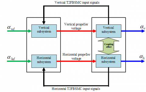
To simplify the synthesis of our controller, we divide the TRMS model into two subsystem models, vertical and horizontal, with 1 degree of freedom each; the coupling effect is considered as uncertainties. We propose to use a decentralized control, that is, from each subsystem model, a T2FBSMC is designed and then the resulting controllers are used to control the TRMS (Figure 9).
Let's start with the vertical subsystem whose model is obtained by the equation (32):
$\left\{ \begin{align} & \dot{x}{{\ }_{1}}\ =\ \ {{x}_{2}} \\ & {{{\dot{x}}}_{2}}=\ \ {{f}_{v}}\left( {{x}_{3}} \right)-{{b}_{v}}\ {{x}_{2}}+{{g}_{v}}\left( {{x}_{1}} \right) \\ & {{{\dot{x}}}_{3}}=\ \ -{{C}_{v\ }}{{x}_{3}}+{{d}_{v}}\ {{u}_{v}} \\ \end{align} \right.$ (58)
where
$\left\{ \begin{align} & \dot{x}{{\ }_{1}}\ =\ \ {{x}_{2}} \\ & {{{\dot{x}}}_{2}}=\ \ {{f}_{v}}\left( {{x}_{3}} \right)-{{b}_{v}}\ {{x}_{2}}+{{g}_{v}}\left( {{x}_{1}} \right) \\ & {{{\dot{x}}}_{3}}=\ \ -{{C}_{v\ }}{{x}_{3}}+{{d}_{v}}\ {{u}_{v}} \\ \end{align} \right.$ (59)
To determine the control law, we proceed in three steps as follows:
Step 1
We define the first error variable ${{z}_{1v}}$ as the tracking error, such as:
${{z}_{1v}}={{x}_{1}}-{{x}_{1d}}={{\alpha }_{v}}-{{\alpha }_{vd}}$ (60)
We define the first function of Lyapunov $V_1v$ by:
${{V}_{1v}}=\frac{1}{2}z_{1v}^{2}$ (61)
The time derivative of (61) is obtained by:
${{\dot{V}}_{1v}}={{z}_{1v}}\ {{\dot{z}}_{1v}}={{z}_{1v}}\left( {{x}_{2}}-{{{\dot{x}}}_{1d}} \right)$ (62)
There is no control input in (38). By letting $x_2$ be the virtual control, the desired virtual control is defined as:
${{\left( {{x}_{2}} \right)}_{d}}=-{{c}_{1v}}{{z}_{1v}}+{{\dot{x}}_{1d}}$ (63)
where, $c_1v$ is a positive constant for increasing the convergence speed of the vertical angle tracking loop.
Now, the virtual control is $x_2$ where the second error tracking is defined by:
${{z}_{2v}}={{x}_{2}}-{{\left( {{x}_{2}} \right)}_{d}}={{x}_{2}}+{{c}_{1v}}{{z}_{1v}}-{{\dot{x}}_{1d}}$ (64)
Step 2
The augmented Lyapunov function for the second step is given by:
${{V}_{2v}}=\frac{1}{2}z_{1v}^{2}+\frac{1}{2}z_{2v}^{2}$ (65)
The derivative of (65) is given by:
${{\dot{V}}_{2v}}=-{{c}_{1v}}z_{1v}^{2}+{{z}_{2v}}{{\dot{z}}_{2v}}$ (66)
Substituting ${{\dot{z}}_{2v}}$ in (66), we obtain:
${{\dot{V}}_{2v}}={{z}_{1v}}\ {{\dot{z}}_{1v}}+{{z}_{2v}}\ \left( {{f}_{v}}\left( {{x}_{3}} \right)-{{b}_{v}}{{x}_{2}}+{{g}_{v}}\left( {{x}_{1}} \right)+{{c}_{1v}}\left( {{x}_{2}}-\dot{x}_{1d}^{{}} \right)-\ddot{x}_{1d}^{{}} \right)$ (67)
By letting ${{f}_{v}}\left( {{x}_{3}} \right)+{{g}_{v}}\left( {{x}_{1}} \right)$ be the virtual control, the desired virtual control in the second step is defined as:
${{\left( {{f}_{v}}\text{ }\left( {{x}_{3}}\text{ } \right)+{{g}_{v}}\text{ }\left( {{x}_{1}}\text{ } \right) \right)}_{d}}=-{{c}_{2v}}\text{ }{{z}_{2v}}+{{b}_{v}}\ {{x}_{2}}-{{c}_{1v}}\text{ }\left( {{x}_{2}}-{{x}_{1d}} \right)+\ddot{x}{}_{1d}$
with
$\left( {{c}_{2v}}>0 \right)$ (68)
Now, the virtual control is $\left( {{c}_{2v}}>0 \right)$ where the sliding surface is defined in the third step by:
${{s}_{v}}={{z}_{3v}}=\left( {{f}_{v}}\left( {{x}_{3}} \right)+{{g}_{v}}\left( {{x}_{1}} \right) \right)-{{\left( {{f}_{v}}\left( {{x}_{3}} \right)+{{g}_{v}}\left( {{x}_{1}} \right) \right)}_{d}}$
$={{f}_{v}}\left( {{x}_{3}} \right)+{{g}_{v}}\left( {{x}_{1}} \right)+{{c}_{2v}}\ {{z}_{2v}}-{{\ddot{x}}_{1d}}+{{c}_{1v}}\left( {{x}_{2}}-{{{\dot{x}}}_{1d}} \right)-{{b}_{v}}\ {{x}_{2}}$ (69)
Step 3
The augmented Lyapunov function for the third step is given by:
${{V}_{3v}}=\frac{1}{2}z_{1v}^{2}+\frac{1}{2}z_{2v}^{2}+\frac{1}{2}s_{v}^{2}$ (70)
The time derivative of (69) is given by:
${{\dot{V}}_{3v}}=z_{1v}^{{}}\dot{z}_{1v}^{{}}+z_{2v}^{{}}\dot{z}_{2v}^{{}}+{{s}_{v}}{{\dot{s}}_{v}}$ (71)
Substituting $s ̇_v$ in (71), we obtain:
${{\dot{V}}_{3v}}=-{{c}_{1v}}\,z_{1v}^{2}-{{c}_{2v}}\,z_{2v}^{2}+{{s}_{v}}\ \left( \frac{\partial \ {{f}_{v}}\left( {{x}_{3}} \right)\ }{\partial {{x}_{3}}}\dot{x}{{}_{3}}+\frac{\partial \ {{g}_{v}}\left( {{x}_{1}} \right)\ }{\partial \ {{x}_{1}}}{{{\dot{x}}}_{1}}+{{c}_{2v}}\left( {{{\dot{x}}}_{2}}+{{c}_{1\ v}}\ \left( {{x}_{2}}-{{{\dot{x}}}_{1\ d}} \right)-{{{\ddot{x}}}_{\ 1\ d}} \right)-{{{}}_{1d}}+{{c}_{1v}}\ \left( {{{\dot{x}}}_{2}}-\ddot{x}{}_{1d} \right)-{{b}_{v}}\ {{{\dot{x}}}_{2}} \right)$ (72)
The chosen low for the attractive surface is the time derivative of (69) stratifying the necessary condition of sliding $(s_v s ̇_v )<0$ obtained in (57):
${{\dot{s}}_{v}}=-{{k}_{fsv}}T2FLC\ \left( {{s}_{v}} \right)$ (73)
As for the proposed T2FBSMC approach, the control input $u_v$ is extracted:
${{u}_{v}}=\frac{1}{{{d}_{v}}\frac{\partial \ {{f}_{v}}\left( {{x}_{3}} \right)}{\partial {{x}_{3}}}}\left[ \begin{align} & {{C}_{v}}\frac{\partial {{f}_{v}}\left( {{x}_{3}} \right)}{\partial {{x}_{3}}}{{x}_{3}}-{{c}_{\ 2v}}\left( {{{\dot{x}}}_{2}}+c{{\ }_{1v}}\ \left( {{x}_{2}}-{{{\dot{x}}}_{1d}} \right)-{{{\ddot{x}}}_{1d}} \right)+{{{}}_{1d}}+\ b{{\ }_{v}}\ \left( {{f}_{v}}\left( {{x}_{3}} \right)-{{b}_{\ v}}\ {{x}_{\ 2}}+g{{\ }_{v}}\ \left( x{{\ }_{1}} \right) \right) \\ & -\frac{\partial {{g}_{v}}\left( {{x}_{1}} \right)}{\partial {{x}_{1}}}{{x}_{2}}-{{c}_{1v}}\ \left( {{{\dot{x}}}_{2}}-\ddot{x}{}_{1d} \right)-{{k}_{fsv}}T2FLC\ \left( {{s}_{v}} \right) \\\end{align} \right]$ (74)
After the design of the proposed T2FBSMC, we must find a control law to reach it and stay thereafter:
${{u}_{v}}={{u}_{eqv}}+{{u}_{rv}}$ (75)
where, $u_eqv$ is the equivalent control. It makes the derivative of the sliding surface equal to zero to stay on the sliding surface. $u_rv$ is the hitting control.
The condition to stay on the sliding surface is $s ̇_v=0$; therefore, the equivalent control is:
${{u}_{eqv}}=\frac{1}{{{d}_{v}}\frac{\partial \ {{f}_{v}}\left( {{x}_{3}} \right)}{\partial {{x}_{3}}}}\left[ {{C}_{v}}\frac{\partial {{f}_{v}}\left( {{x}_{3}} \right)}{\partial {{x}_{3}}}{{x}_{3}}-{{c}_{2v}}\left( {{{\dot{x}}}_{2}}+{{c}_{1v}}\ \left( {{x}_{2}}-{{{\dot{x}}}_{1d}} \right)-{{{\ddot{x}}}_{1d}} \right)+{{{}}_{1d}}+\ b{{\ }_{v}}\ \left( {{f}_{v}}\left( {{x}_{3}} \right)-{{b}_{\ v}}\ {{x}_{\ 2}}+g{{\ }_{v}}\ \left( x{{\ }_{1}} \right) \right)-... \right.$
$\left. \frac{\partial {{g}_{v}}\left( {{x}_{1}} \right)}{\partial {{x}_{1}}}{{x}_{2}}-{{c}_{1v}}\ \left( {{{\dot{x}}}_{2}}-\ddot{x}{}_{1d} \right) \right]$(76)
${{u}_{rv}}=-\,\left( \frac{{{k}_{fsv}}}{{{d}_{v}}\frac{\partial \ {{f}_{v}}\left( {{x}_{3}} \right)}{\partial {{x}_{3}}}} \right)T2FLC\ \left( {{s}_{v}} \right)$ (77)
where $k_{fsv}$ is a positive constant.
Similar to the vertical subsystem case, the control law $u_h$ for the horizontal subsystem is:
${{u}_{h}}={{u}_{eqh}}+{{u}_{rh}}$ (78)
$u{{}_{h}}\ =\ \frac{1}{{{d}_{h}}\frac{\partial {{f}_{h}}\left( {{x}_{6}} \right)}{\partial {{x}_{6}}}}\,\,\left[ {{C}_{h}}\frac{\partial {{f}_{h}}\left( x{{}_{6}} \right)}{\partial {{x}_{6}}}{{x}_{6}}-{{c}_{\ 2h}}\ \left( {{{\dot{x}}}_{5}}+c{{\ }_{1h}}\ \left( {{x}_{5}}-{{{\dot{x}}}_{4d}} \right)-{{{\ddot{x}}}_{4d}} \right)+{{}_{4d}}\ +b{{\ }_{h}}\ \left( {{f}_{h}}\left( {{x}_{6}} \right)-{{b}_{\ h}}\ {{x}_{\ 5}} \right)-{{c}_{1\ h}}\ \left( {{{\dot{x}}}_{5}}-\ddot{x}\ {}_{4d} \right)-... \right.$
$\left. {{k}_{fsh}}T2FLC\ \left( {{s}_{h}} \right) \right]$(79)
With:
\[\left( {{c}_{1h}},{{c}_{2h\text{ }}} \right)>0\text{ }and\text{ }{{s}_{h}}={{z}_{3h}}={{f}_{h}}\left( {{x}_{6}} \right)+{{c}_{2h}}{{z}_{2h}}-\ddot{x}{{\text{ }}_{4d}}+{{c}_{1h}}\left( {{x}_{5}}-{{{\dot{x}}}_{4d}} \right)-{{b}_{h}}\ {{x}_{5}}\]
The equivalent control for the horizontal subsystem is:
$u{{}_{eqh}}\ =\ \frac{1}{{{d}_{h}}\frac{\partial {{f}_{h}}\left( {{x}_{6}} \right)}{\partial {{x}_{6}}}}\,\,\left[ {{C}_{h}}\frac{\partial {{f}_{h}}\left( x{{}_{6}} \right)}{\partial {{x}_{6}}}{{x}_{6}}-{{c}_{2h}}\ \left( {{{\dot{x}}}_{5}}+c{{\ }_{1h}}\ \left( {{x}_{5}}-{{{\dot{x}}}_{4d}} \right)-{{{\ddot{x}}}_{4d}} \right)+{{{}}_{4d}}\ +b{{\ }_{h}}\ \left( {{f}_{h}}\left( {{x}_{6}} \right)-{{b}_{\ h}}{{x}_{\ 5}} \right)-{{c}_{1\ h}}\ \left( {{{\dot{x}}}_{5}}-\ddot{x}\ {}_{4d} \right) \right]$ (80)
and for the following corrective control
${{u}_{rh}}\ =-\ \left( \frac{{{k}_{fsh}}}{{{d}_{h}}\frac{\partial {{f}_{h}}\left( {{x}_{6}} \right)}{\partial {{x}_{6}}}} \right)\,\,T2FLC\ \left( {{s}_{h}} \right)$ (81)
The bloc diagram of the proposed T2FBSMC is shown in Figure 9.
Figure 9. Block diagram of the proposed T2FBSMC
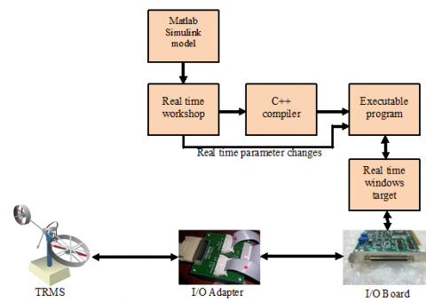
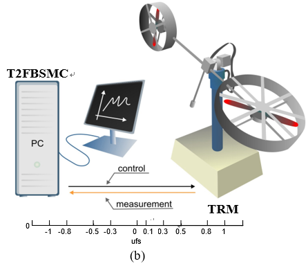
Our controller was implemented using Simulink, a graphical programming language tool developed by MathWorks. The control system flow diagram is shown in Figure 10. The Simulink model is transferred to Real-Time Workshop (RTW) to build a C++ source program. C++ compiler compiles and links this program to produce an executable code. Real-Time Windows target is used as an interface between the created executable program acting as the control program and the input/output (I/O) board [15, 11].
Figure 10. Experimental environment of the TRMS [15]
The complete set up of TRMS platform is shown in Figure 11. The system consists of [15]
Figure 11. TRMS platform experiment [15]
PCI 1711 Lab is a universal Feedback unit having two blocks, Feedback encoder block and Feedback DAC block. For the TRMS two encoders are used thus the values of the $α_v$ and $α_h$ are returned in Feedback encoder block. There are three parameters for this block: sample time, i.e. 0.001 sec, channel one and channel two offsets. Channel one refers to the first encoder output $α_v$ and channel two to the second encoder output $α_h$. The digital input value given to PCI1711 is converted to analog output by Feedback DAC block.
6.1 Tracking control experiment of square wave response
Figure 12 (a and b) illustrates the responses of the control system according to square reference signals for pitch and yaw angles which show the ability of the proposed control system in the tracking problem. In addition, Figure 12 (c and d), indicate that the actual control voltage $u_ψ$ and $u_φ$ for main and tail DC motors are confined in the permitted interval of [-2.5, 2.5] volts and the chattering effect is eliminated. It is clear here that the peaking phenomena occurred in control signals is due to the discontinuous nature of the challenging square reference signals.
Figure 12. Experimental results of the square signal tracking
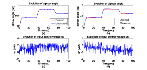
6.2 Tracking control experiment of high speed trajectory
The tracking responses experiment are shown in Figure 13 (a and b). From the results, it is noted that the proposed controller can result in great tracking responses. On the other hand, from Figure 13 (c and d), it can be seen that the control signals are quite smooth and the actual control input voltages for main and tail DC motors are confined in the permitted interval of [-2.5, 2.5] volts. In all test cases, the controller is efficient to maintain the angles close to their desired values after transient deviations.
Figure 13. Experimental results of the high speed trajectory tracking
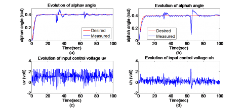
6.3 Robustness to the external disturbances
Figure 14. Step responses of the TRMS with the proposed T2FBSMC controller subject to the external disturbance
To evaluate the robustness of the proposed T2FBSMC controller, an external disturbance were introduced to the system at t=30s and t=64s. The experiment results are depicted in Figure14 (a and b) which shows that the controller is immune recovers adequately for the external perturbation. The peaking phenomenon appears in the input voltages uv and uh , as shown in Figure 14 (c and d), represents the transient of the adaptation to compensate the sudden change of TRMS angles caused by perturbation.
Our controller was implemented using Simulink, a graphical programming language tool developed by MathWorks. The control system flow diagram is shown in Figure 10. The Simulink model is transferred to Real-Time Workshop (RTW) to build a C++ source program. C++ compiler compiles and links this program to produce an executable code. Real-Time Windows target is used as an interface between the created executable program acting as the control program and the input/output (I/O) board [15, 11].
This paper addressed the design of real time implementation of T2FBSMC for a TRMS system in the presence of external disturbances. Firstly, we start by the development of the dynamic model of the TRMS taking into account the different physics phenomena. A highly coupled nonlinear TRMS is decomposed into a set of main and tail subsystems with the coupling effect considered as the uncertainties. Simulation and experimental results are presented to show the effectiveness of the proposed method. In addition the comparative study performed with other works developed in the literature, has shown the effectiveness of the proposed control approach.
[1] Bouguerra A, Saigaa D, Kara K, Zeghlache S. (2015). Fault-tolerant Lyapunov-gain-scheduled PID control of a quadrotor UAV. International Journal of Intelligent Engineering and Systems 8(2): 1-6. https://doi.org/10.22266/ijies2015.0630.01
[2] Zeghlache S, Amardjia N. (2018). Real time implementation of non linear observer-based fuzzy sliding mode controller for a twin rotor multi-input multi-output system (TRMS). Optik 156: 391-407. https://doi.org/10.1016/j.ijleo.2017.11.053
[3] Ahmad SM. (2001). Modelling and control of a twin rotor MIMO system. University of London.
[4] Castillo P, Lozano R, Dzul AE. (2006). Modelling and control of mini-flying machines. Springer-Verlag London.
[5] Chalupa P, Přikryl J, Novák J. (2015). Modelling of twin rotor MIMO system. Procedia Engineering 100: 249-258. https://doi.org/10.1016/j.proeng.2015.01.365
[6] Edwards C, Spurgeon K. (1998). Sliding mode control: Theory and applications. CRC Press.
[7] Ramy R, Ayman E, Ahmed A. (2017). Sliding mode disturbance observer-based of a twin rotor MIMO system. ISA transactions 69: 166-174. https://doi.org/10.1016/j.isatra.2017.04.013
[8] Ekbote AK, Srinivasan NS, Mahindrakar AD. (2011). Terminal sliding mode control of a twin rotor multiple-input multiple-output system. IFAC Proceedings Volumes 44(1): 10952-10957. https://doi.org/10.3182/20110828-6-IT-1002.00645
[9] Mondal S, Mahanta C. (2012). Adaptive second-order sliding mode controller for a twin rotor multi-input-multi-output system. IET on Control Theory & Applications 6(14): 2157-2167. https://doi.org/10.1049/iet-cta.2011.0478
[10] Yu GR, Liu HT. (2005). Sliding mode control of a two-degree-of freedom helicopter via linear quadratic regulator. 2005 IEEE International Conference on Systems, Man and Cybernetics 4: 3299-3304. https://doi.org/10.1109/ICSMC.2005.1571655
[11] Faris F, Moussaoui A, Boukhetala D, Tadjine M. (2017). Design and real-time implementation of a decentralized sliding mode controller for twin rotor multi-input multi-output system. Journal of Systems and Control Engineering 231: 3-13. https://doi.org/0.1177/0959651816680457
[12] Zeghlache S, Kara K, Saigaa D. (2014). Type-2 fuzzy logic control of a 2-DOF helicopter (TRMS system). Open Engineering 4(3): 303-315. https://doi.org/10.2478/s13531-013-0157-y
[13] Maouche D, Eker I. (2017). Adaptive fuzzy type-2 in control of 2-DOF helicopter. International Journal of Electronics and Electrical Engineering 5: 99-105. https://doi.org/10.18178/ijeee.5.2.99-105
[14] Shaik FA, Purwar S. (2009). A nonlinear state observer design for 2 – DOF twin rotor system using neural networks. 2009 International Conference on Advances in Computing, Control, and Telecommunication Technologies, pp. 15-19. https://doi.org/10.1109/ACT.2009.219
[15] Rotor MT. (1997). System Advanced Technique Manual. Feedback Instruments Ltd.
[16] Liang Q, Mendel J. (2000). Interval type-2 fuzzy logic systems: theory and design. IEEE Transactions on Fuzzy Systems 8: 535-550. https://doi.org/10.1109/91.873577
[17] Mendel JM. (2001). Uncertain rule-based fuzzy logic systems: Introduction and new directions. Prentice-Hall.
[18] Castillo O, Melin P. (2012). A review on the design and optimization of interval type-2 fuzzy controllers. Applied Soft Computing 12(4): 1267-1278. https://doi.org/10.1016/j.asoc.2011.12.010
[19] Juan R, Castillo O, Melin P, Rodríguez-Díaz A. (2009). A hybrid learning algorithm for a class of interval type-2 fuzzy neural networks. Information Sciences 179(13): 2175-2193. https://doi.org/10.1016/j.ins.2008.10.016
[20] Martínez R, Castillo O, Aguilar L. (2009). Optimization of interval type-2 fuzzy logic controllers for a perturbed autonomous wheeled mobile robot using genetic algorithms. Information Sciences 179(13): 2158–2174. https://doi.org/10.1016/j.ins.2008.12.028
[21] Wu D, Tan WW. (2006). A simplified type-2 fuzzy logic controller for real-time control. ISA Transactions 45(4): 503-51. https://doi.org/10.1016/S0019-0578(07)60228-6
[22] Castillo O, Marroquín M, Melin P, Valdez F, Soria J. (2010). Comparative study of bio-inspired algorithms applied to the optimization of type-1 and type-2 fuzzy controllers for an autonomous mobile robot. Information Sciences 192: 19-38. https://doi.org/10.1016/j.ins.2010.02.022
[23] Zhou Y, Wu Y, Hu Y. (2007). Robust backstepping sliding mode control of a class of uncertain MIMO nonlinear systems. 2007 IEEE International Conference on Control and Automation, pp. 1916-1921. https://doi.org/10.1109/ICCA.2007.4376695
[24] Zeghlache S, Kamel K, Djamel S. (2015). Fault tolerant control based on interval type-2 fuzzy sliding mode controller for coaxial trirotor aircraft. ISA Transaction 59: 215-231. https://doi.org/10.1016/j.isatra.2015.09.006