Mario A. Cucumo* | Vittorio Ferraro | Dimitrios Kaliakatsos | Francesco Nicoletti | Albino Gigliotti
OPEN ACCESS
In this study, the thermal and electrical modeling of a photovoltaic panel is performed to evaluate its temperature profiles, electrical efficiency and the electrical power supplied. The energy balance equations under transient conditions of all the layers that make up the panel are discretized by the finite difference technique and solved with the implicit method. The results are validated with experimental data provided by an experimental set-up located on the roof of a building of the Department of Mechanical, Energy and Management Engineering (DIMEG) of the University of Calabria. The comparison with the experimental data allows us to see an excellent approximation of the distribution of temperatures inside the panel and in particular of the photovoltaic cells, accurately evaluating the effect on electrical efficiency and the electrical power supplied. The validation was performed with reference to a clear winter day and a clear summer day. The mean square error was about 1.5°C on the panel temperature and about 3 W on the electrical power (1.2% of the maximum power).
finite differences, PV producibility, predictive method
An accurate estimate of the temperature of photovoltaic panels is essential to assess their electrical performance. Therefore, in this work, one of the main objectives is to illustrate a simple and very accurate method for predicting the temperature of the PV panels, on which the electrical power supplied and the electrical efficiency depend.
Being able to predict the producibility of a photovoltaic field is becoming increasingly important for their interconnection within smart-grids [1]. In these networks, on which investments are being made for the future, it is necessary to estimate the electrical loads, the electrical generations and the electrical storage systems installed in a decentralized manner on the territory [2-4]. Consequently, the prediction of the behavior of small-scale systems also becomes important [5], especially as regards plants that use renewable sources with high variability of the primary source.
In this work, a calculation model will be developed and validated with a photovoltaic panel installed at the DIMEG of the University of Calabria. Bevilacqua et al. [6] have validated their calculation method on the same photovoltaic system. They developed a finite difference model by defining many nodes within the panel. In the present work, with a similar methodology, we want to investigate the possibility of obtaining good results with a simpler finite difference model, defining only 5 nodes, as also proposed by Notton et al. [7].
In the literature there are several models to estimate the electrical producibility of a photovoltaic panel.
The technique applied in this study consist in a non-stationary model, therefore able to also consider capacitive effects and reliably simulate the operating conditions relating, for example, to the passage of a cloud or to abrupt local climatic variations [8, 9].
Several scientific papers investigate the link between electrical efficiency and climatic variables such as irradiance and temperature. Chaibi et al. [10] analyzes the current/voltage (I-V) characteristics for Si-crystalline PV modules under non-standard condition by using single-diode and double-diode models. Rodziewicz et al. [11] analyzes the influence of changes in the solar radiation spectrum distribution on the properties of various photovoltaic modules, with particular emphasis on the scattered component.
A complex fluid dynamics calculation model was developed by Jaszczur et al. [12]. However, the calculation requires a computational effort and is not easy to use.
The aim of this paper will be to use a simpler procedure for estimating the quantities of interest, but with still accurate results.
The thermal model developed in the present study has two functions: the first is to estimate the temperature of the photovoltaic cells, which is used to predict the electrical energy production which varies with operating conditions; secondly, it provides the temperatures in the different layers along the thickness of the photovoltaic panel, which helps to better understand the function of each of them in heat dissipation. After having analyzed numerous other scientific articles on this topic [13-17], the correlation used to estimate the electrical efficiency is the Evans equation [18]. In this equation the most important term is the PV temperature. Therefore, it is necessary to determine it precisely.
The idea is to carry out the calculations, in a transient manner, as a function of solar irradiation, temperature, wind speed, relative humidity [19] in order to be used for predictive purposes.
The photovoltaic panel considered in this study is the model Schüco MPE 245 PG 60 FA. It is made up of 60 (6x10) polycrystalline cells in series, for a total panel size of 1663x998 mm.
The manufacturer declares a maximum yield in reference conditions of 14.5% in standard conditions.
The layers considered for the physical model from top to bottom are: glass, upper EVA (Ethylene Vinyl Acetate), PV cells, lower EVA and Tedlar (polyvinyl fluoride). In modeling the upper and lower EVA layers, which enclose the central layer of the PV cells, are considered separately but with the same physical and thermal properties. The physical and thermal properties of each layer are given in Table 1.
Table 1. Thermophysical properties of the layers
|
Layer |
Thickness s (mm) |
Thermal conductivity k (W/mK) |
Density ρ (kg/m3) |
Specific Heat c (J/kgK) |
|
Glass |
3.2 |
1.8 |
3000 |
500 |
|
Upper EVA |
0.2 |
0.35 |
960 |
2090 |
|
PV cells |
0.3 |
148 |
2330 |
677 |
|
Lower EVA |
0.2 |
0.35 |
960 |
2090 |
|
Tedlar |
0.1 |
0.2 |
1200 |
1250 |
In the thermal model, the photovoltaic panel is divided into five separate layers, for each of them a point is considered and the energy conservation equations are written in the form of thermal balance equations. Starting from top to bottom, the first point in the glass layer is taken on the surface and has a temperature $T_{f g}$; the second point in the middle of the upper EVA layer has a temperature $T_{e v, s u p}$, the third point in the center of the panel and the PV cell layer has a temperature $T_{p v}$, the fourth in the center of the lower EVA layer has a temperature $T_{e v, s u p}$ and, finally, the fifth point is located on the lower surface of the tedlar layer and has a temperature $T_{\text {ted }}$. Figure 1 shows the layers with their thicknesses and the point temperatures for each layer.
Figure 1. Subdivision into layers of the PV panel and nodes
For each node the relative thermal balance equation can be written taking into account the conductive resistances between each of them, the convective and radiative resistances at the boundary, the accumulated thermal power and the absorbed thermal power.
The conductive resistances of each layer are indicated with $R_{i}=\frac{s_{i}}{k_{i} A_{i}}$ with reference to the whole thickness s. The resistance of half the thickness of the layer is indicated with $\frac{1}{2} R_{i}$, accordingly. The equations for the five nodes are:
$\frac{T_{a}-T_{f g}}{R_{\text {conv }}}+\frac{T_{s k y}-T_{f g}}{R_{r a d, f g-s k y}}+\frac{T_{g r}-T_{f g}}{R_{r a d, f g-g r}}+\frac{T_{e v, s u p}-T_{f g}}{R_{f g}+\frac{1}{2} R_{e v}}+\dot{Q}_{f g}=\rho_{f g} c_{f g} V_{f g} \frac{d T_{f g}}{d t}$ (1)
$\frac{T_{f g}-T_{e v, \text { sup }}}{R_{f g}+\frac{1}{2} R_{e v}}+\frac{T_{p v}-T_{e v, s u p}}{\frac{1}{2} R_{e v}+\frac{1}{2} R_{p v}}=\rho_{e v} c_{e v} V_{e v} \frac{d T_{e v, \text { sup }}}{d t}$ (2)
$\frac{T_{e v, s u p}-T_{p v}}{\frac{1}{2} R_{e v}+\frac{1}{2} R_{p v}}+\frac{T_{e v, i n f}-T_{p v}}{\frac{1}{2} R_{p v}+\frac{1}{2} R_{e v}}+\dot{Q}_{p v}=\rho_{p v} c_{p v} V_{p v} \frac{d T_{p v}}{d t}$ (3)
$\frac{T_{p v}-T_{e v, i n f}}{\frac{1}{2} R_{p v}+\frac{1}{2} R_{e v}}+\frac{T_{t e d}-T_{e v, i n f}}{\frac{1}{2} R_{e v}+R_{t e d}}=\rho_{e v} c_{e v} V_{e v} \frac{d T_{e v, i n f}}{d t}$ (4)
$\frac{T_{a}-T_{t e d}}{R_{\text {conv }}}+\frac{T_{s k y}-T_{\text {ted }}}{R_{\text {rad,ted-sky }}}+\frac{T_{g r}-T_{t e d}}{R_{\text {rad,ted }-g r}}+\frac{T_{e v, i n f}-T_{t e d}}{\frac{1}{2} R_{e v}+R_{t e d}}=\rho_{t e d} c_{t e d} V_{t e d} \frac{d T_{t e d}}{d t}$ (5)
The total solar radiation absorbed in the PV cells is calculated by means of radiation models and, in the literature, there are several available [20, 21].
The formula proposed by Aly et al. [22] which has been validated with experimental results is:
$\dot{Q}_{p v}=\alpha_{P V} \cdot \tau(i) \cdot G \cdot A \cdot\left(1-\eta_{p v}\right)$ (6)
in which $\alpha_{P V}$ is the effective absorption coefficient of the photovoltaic cells, which in our case assumes a value equal to 0.93 [23]; G is the total radiation incident on the inclined plane of the PV panel, τ(i) is the transmission coefficient of the front glass for the direct component which depends on the angle of incidence i. The latter is obtained from the following formula [24].
$\tau(i)= e^{-\left(\frac{K \cdot s_{f g}}{\cos i_{r}}\right)}\left[1-\frac{1}{2}\left(\frac{\sin ^{2}\left(i_{r}-i\right)}{\sin ^{2}\left(i_{r}+i\right)}+\frac{\tan ^{2}\left(i_{r}-i\right)}{\tan ^{2}\left(i_{r}+i\right)}\right)\right]$ (7)
in which K is the extinction constant of the glass, which assumes a value of 4 m-1 in the case of tempered glass used in PV panels [20], $i_{r}$ is the refraction angle of the direct radiation incident through the glass and can be derived from Snell's law [20].
The last term of Eq. (6) represents the inefficiency of converting solar energy into electricity as $\eta_{p v}$ is the yield of the PV cells. The latter depends on the temperature of the cells $T_{P V}$ and by irradiance G:
$\eta_{p v}=\eta_{p v, r e f} \cdot\left[1-\beta_{r e f}\left(T_{p v}-T_{r e f}\right)+\gamma \log _{10} \frac{G}{1000}\right]$ (8)
with $\beta_{r e f}=0.006^{\circ} \mathrm{C}^{-1}$ and $\gamma=0.085$ for the PV panel (Tonui and Tripanagnostopoulos [25]) and $T_{\text {ref }}=25^{\circ} \mathrm{C}$.
The thermal power absorbed by the glass is equal to:
$\dot{Q}_{f g}=\alpha_{f q} \cdot G \cdot A$ (9)
in which $\alpha_{f g}=0.05$ is the absorption coefficient of the front glass.
To solve the problem, the technique of finite differences FD with respect to time is used. The calculations will then be carried out with the aid of a simple spreadsheet (Microsoft Excel). For each instant in time, the incoming data are the total radiation incident on the surface of the photovoltaic panel, the ambient temperature and the wind speed. First of all, the equations are rewritten by dividing both sides of each equation by the surface area of the corresponding layer and discretizing the time derivative referring it to finite time intervals:
$h_{\text {conv }}\left(T_{a}-T_{f g}\right)+h_{r a d, f g-s k y}\left(T_{s k y}-T_{f g}\right)+\frac{T_{e v, \text { sup }}-T_{f g}}{\frac{s_{f g}}{k_{f g}}+\frac{1}{2} \frac{s_{e v}}{k_{e v}}}+h_{r a d, f g-g r}\left(T_{g r}-T_{f g}\right)+\alpha_{f g} G=\rho_{f g} c_{f g} s_{f g} \frac{T_{f g}-T_{f g}^{p}}{\Lambda t}$ (10)
$\frac{T_{f g}-T_{e v, \sup }}{\frac{s_{f g}}{k_{f g}}+\frac{1}{2} \frac{s_{e v}}{k_{e v}}}+\frac{T_{p v}-T_{e v, s u p}}{\frac{1}{2} \frac{s_{e v}}{k_{e v}}+\frac{1}{2} \frac{s_{p v}}{k_{p v}}}=\rho_{e v} c_{e v} s_{e v} \frac{T_{e v, s u p}-T_{e v, s u p}^{p}}{\Delta t}$ (11)
$\frac{T_{e v, s u p}-T_{p v}}{\frac{1}{2} \frac{s_{e v}}{k_{e v}}+\frac{1}{2} \frac{s_{p v}}{k_{p v}}}+\frac{T_{e v, i n f}-T_{p v}}{\frac{1}{2} \frac{s_{p v}}{k_{p v}}+\frac{1}{2} \frac{s_{e v}}{k_{e v}}}+\alpha_{P V} \cdot \tau(i) \cdot G \cdot\left(1-\eta_{P V}\right)=\rho_{p v} c_{p v} s_{p v} \frac{T_{p v}-T_{p v}{ }^{p}}{\Delta t}$ (12)
$\frac{T_{p v}-T_{e v, i n f}}{\frac{1}{2} \frac{s_{p v}}{k_{p v}}+\frac{1}{2} \frac{s_{e v}}{k_{e v}}}+\frac{T_{t e d}-T_{e v, i n f}}{\frac{1}{2} \frac{s_{e v}}{k_{e v}}+\frac{s_{t e d}}{k_{t e d}}}=\rho_{e v} c_{e v} s_{e v} \frac{T_{e v, i n f}-T_{e v, i n f}^{p}}{\Delta t}$ (13)
$h_{\text {conv }}\left(T_{a}-T_{t e d}\right)+h_{\text {rad,ted-sky }}\left(T_{s k y}-T_{\text {ted }}\right)+\frac{T_{e v, i n f}-T_{t e d}}{\frac{1}{2} \frac{s_{e v}}{k_{e v}}+\frac{s_{t e d}}{k_{t e d}}}+h_{r a d, t e d-g r}\left(T_{g r}-T_{t e d}\right)=\rho_{t e d} c_{t e d} s_{t e d} \frac{T_{t e d}-T_{t e d}^{p}}{\Delta t}$ (14)
In the equations, all temperatures and variables refer to the present time t, while temperatures with apex p refer to the previous time $t-\Delta t$.
For natural convection the Nusselt number is calculated as if the plate were horizontal, with the following expression for the top surface [26]:
$N u_{\text {conv, free }}=0.13 \cdot R a^{\frac{1}{3}}$ (15)
And the following for the lower surface [27]:
$N u_{\text {conv, free }}=0.27 \cdot R a^{\frac{1}{4}}$ (16)
The Rayleigh number is calculated using the average length of the two panel dimensions.
For forced convection, in turbulent outflow, the Nusselt number is calculated with the following relation due to Sparrow [28]:
$N u_{\text {conv,forced }}=0.86 \cdot R e_{L, c}^{\frac{1}{2}} \cdot P r^{\frac{1}{3}}$ (17)
The Reynolds number is calculated at the characteristic length $L_{c}$ which is four times the plate area divided by the perimeter. It is not a length that considers the wind direction.
When the flow is laminar, however, it is preferred to use the classical expression coming from the boundary layer theory [29]:
$N u_{\text {conv,forced }}=0.664 \cdot R e_{Lc}^{\frac{1}{2}} \cdot \operatorname{Pr}^{\frac{1}{3}}$ (18)
The overall value of the convection is calculated taking into account the combined natural and forced flow and is estimated using the Churchill expression [30]:
$h_{\text {conv }}=\sqrt[3]{{h_{\text {conv,free }}}^{3}+{h_{\text {conv,forced }}}^{3}}$ (19)
Many authors in the scientific literature, such as Notton et al. [7] and Barroso et al. [31], use the formulas of the coefficients of heat transmission by radiation, both for the upper and lower surfaces, in linearized form. In our model, to be more precise, we will use the exact non-linearized formulas and apply them separately for both surfaces:
$h_{r a d, i-s k y / g r}=\frac{\sigma \cdot\left(T_{i}^{2}+T_{s k y / g r}^{2}\right)\left(T_{i}+T_{s k y / g r}\right)}{\frac{1-\varepsilon_{i}}{\varepsilon_{i}}+\frac{1}{F_{i-s k y / g r}}}$ (20)
in which $T_{i}$ is the surface temperature of the outer layer for which we want to calculate the heat exchange coefficient, $T_{s k y / g r}$ represents the temperature of the celestial vault or the temperature of the ground. The temperature of the celestial vault can be calculated with the following formula [32], widely used in scientific literature:
$T_{s k y}=0.0552 \cdot T_{a}^{1.5}$ (21)
where $T_{a}$ is the air temperature.
The ground temperature can be set equal to the ambient temperature:
$T_{g r}=T_{a}$ (22)
The view factors are:
$F_{f g-s k y}=F_{t e d-g r}=\frac{1+\cos \beta}{2}$ (23)
$F_{f g-g r}=F_{t e d-s k y}=\frac{1-\cos \beta}{2}$ (24)
$\varepsilon_{f g}$ is the emissivity of the glass for which various values have been proposed in the scientific literature including 0.86 proposed by Hegazy [33] and 0.85 by Notton et al. [7] taken from experimental tests verified and disclosed by the manufacturer Photowatt. We will use the latter value. For the lower surface of the tedlar $\varepsilon_{\text {ted }}$ will be taken equal to 0.85.
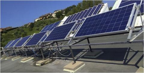
The experimental setup, to which we will refer for the validation of the theoretical models, is located on the roof of a building of the Department of Mechanical, Energy and Management Engineering (DIMEG) of the University of Calabria (latitude 39.37°N, longitude 16.23°E) and is represented by a photovoltaic panel anchored to an aluminum structure that provides an inclination of 30°with orientation to the South, as shown in Figure 2. The temperature is measured with a sensor placed on the back of the panel.
Figure 2. Experimental apparatus on the roof of a building of the DIMEG department at Unical [6]
4.1 Validation in winter conditions
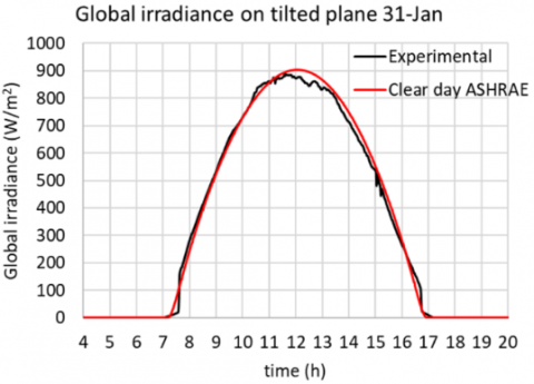
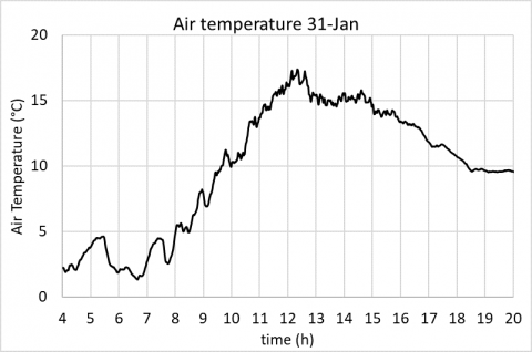
As an example, the results are shown for the day of January 31th, which represents a winter day in which clear sky conditions were detected, as observed in Figure 3. This figure shows the comparison between the global radiation measured on the plane of the panel with the radiation evaluated by the ASHRAE clear day model [34]. The two curves are almost coincident. Figure 4 shows the outside air temperature; Figure 5 shows the wind speed, which is moderate until 12:30 and intensifies after this time.
Figure 3. Global irradiance on January 31th
Figure 4. Air temperature on January 31th
Figure 5. Wind speed on January 31th
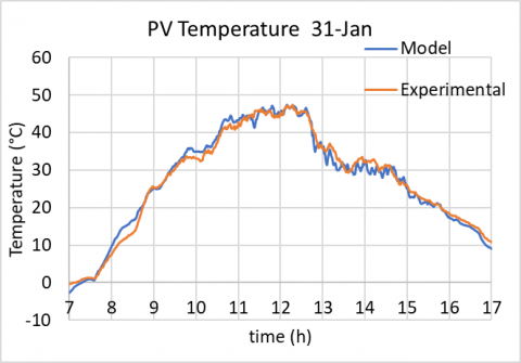
The temperature of the tedlar is compared with the temperature measured experimentally in Figure 6. In particular, the temperature reaches a maximum value around noon of 47.4°C. It is noted that the temperature obtained through the model almost perfectly approximates the temperature measured experimentally. This qualitative consideration is supported by the statistical parameters (Table 2) and, in particular, by the correlation coefficient which assumes the value CC = 0.996, which denotes an excellent correlation, and by the Nash-Sutcliffe efficiency which assumes the value of NSE = 0.989, which denotes very good model accuracy. The MBE represents the Mean Bias Error. It is slightly negative and indicates a slight underestimation of the modeled data compared to the experimental ones. The RSME mean square error is about 1.7°C.
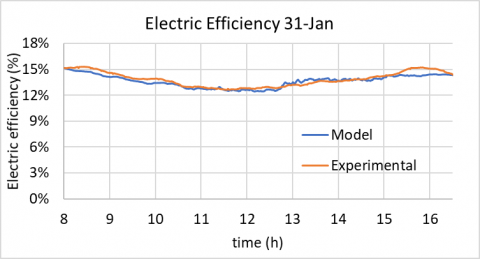
Figure 7 shows the comparison between the electrical efficiency estimated by the model and the experimental one. Also in this case, the statistical indices show an excellent behavior of the model.
Figure 6. Photovoltaic temperature. Model vs experimental data. January 31th
Table 2. Correlation indexes for Photovoltaic temperature. January 31th
|
CC |
MBE (°C) |
RMSE (°C) |
NSE |
|
0.996 |
-0.602 |
1.694 |
0.989 |
Figure 7. Electric efficiency. Model vs experimental data. January 31th
Table 3. Correlation indexes for Electric efficiency. January 31th
|
CC |
MBE (%) |
RMSE (%) |
NSE |
|
0.9994 |
-0.081 |
0.268 |
0.998 |
In Figure 8, on the other hand, the graphs of the modeled electric power and the one measured experimentally are represented on the same diagram. Table 4 highlights the statistical parameters mentioned above.
What has been said for the temperature also applies to the modeled electrical power: the trend is well represented and this is confirmed by the statistical parameters with CC = 0.9995, which denotes an excellent correlation and NSE = 0.999. In this case, the MBE is slightly negative at just half a Watt.
Figure 8. Electric power. Model vs experimental data. January 31th
Table 4. Correlation indexes for Electric power. January 31th
|
CC |
MBE (W) |
RMSE (W) |
NSE |
|
0.9995 |
-0.512 |
2.476 |
0.999 |
The maximum electrical power has a value of approximately 185.2 W which is lower than the maximum rated electrical power that can be delivered as the irradiance is not 1000 W/m2 and the cell temperature is much higher than the reference temperature.
4.2 Validation in summer conditions
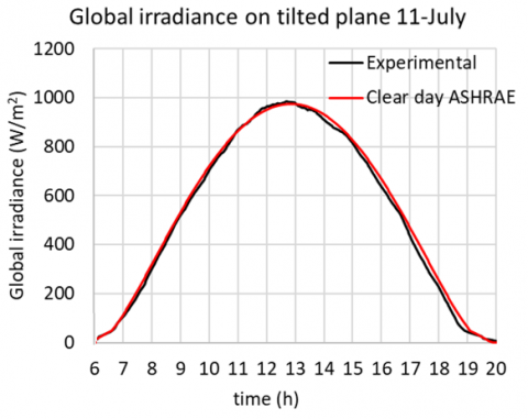
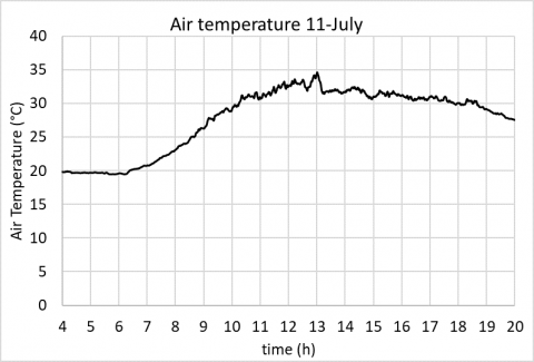
With reference to July 11th, Figure 9 shows the comparison between the global radiation measured on the panel plane with the radiation evaluated by the ASHRAE clear day model. Figure 10 shows the air temperature, while Figure 11 shows the wind speed.
Figure 9. Global irradiance on July 11th
Figure 10. Air temperature on July 11th
Figure 11. Wind speed on July 11th
Figure 12 shows the comparison between measured temperature and obtained from the model. The trend appears to be well represented by the model. The maximum temperature reached has a value of about 65°C around 13.00. it is possible to observe a reduction in temperature in the afternoon due to the increase in wind speed. The model therefore demonstrates to perform well with a correlation index of 0.996 and an NSE of 0.99 (Table 5). Even from a visual analysis, it is clear that there are no deviations between the trends both when the wind speed is low and when it generates a turbulent motion. Again, there is an underestimate of about half a degree Celsius and an RMSE of about 1.4°C.
The efficiency is shown in Figure 13. The RMSE is 0.239% (Table 6).
Figure 12. Photovoltaic temperature. Model vs experimental data. July 11th
Table 5. Correlation indexes for Photovoltaic temperature. July 11th
|
CC |
MBE (°C) |
RMSE (°C) |
NSE |
|
0.996 |
-0.513 |
1.442 |
0.990 |
Figure 13. Electric efficiency. Model vs experimental data. July 11th
Table 6. Correlation indexes for Electric efficiency. July 11th
|
CC |
MBE (%) |
RMSE (%) |
NSE |
|
0.94 |
0.077 |
0.239 |
0.987 |
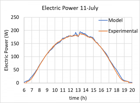
The electric power (Figure 14) is slightly overestimated, especially at the moment of maximum production. However, the RMSE is about 3.39 W (Table 7) on a peak power of about 180 W.
Figure 14. Electric power. Model vs experimental data. July 11th
Table 7. Correlation indexes for Electric power. July 11th
|
CC |
MBE (W) |
RMSE (W) |
NSE |
|
0.9992 |
1.713 |
3.391 |
0.998 |
Figure 15 shows the temperature profile obtained through the model inside the PV panel at noon on July 11th. The model allows to determine the temperatures at the centroids of the EVA and PV layers. Knowing the conductive thermal resistances of the individual layers, the temperatures at the interfaces of the layers are also easily identifiable.
Figure 15. Temperature Profile. July 11th. 12:00
In this figure it can be observed that the temperature in the layer of the photovoltaic cells is almost constant, due to its high thermal conductivity and reaches the maximum value of 62.12°C. The temperature decreases going towards the external surfaces and assumes a value of 61.29°C on the upper surface of the glass and a value of 61.81°C on the lower surface of the tedlar. Taking into account that the characteristics of the EVA layers on the sides of the PV cell layer are identical, the different temperature on the external surfaces can be explained by the fact that the glass layer has a thermal conductivity 9 times greater than that of the tedlar layer ($k_{f g}=1.8 \frac{w}{m \cdot K}$ and $k_{t e d}=0.2 \frac{w}{m \cdot K}$) but it also has a much larger thickness of 32 times ($s_{f g}=3.2 \mathrm{~mm}$ and $s_{t e d}=0.1 \mathrm{~mm}$) and, therefore, the conductive thermal resistance is greater.
The aim of the work was the thermal modeling of a photovoltaic panel to analyze its performance, for example for predictive purposes. The physical and optical-radiative modeling of the photovoltaic panel made it possible to evaluate the spatial and temporal temperature profile within the PV. In particular, the convective and radiative exchanges were estimated for both the upper and lower surfaces with the relative view factors, evaluating the most accurate and reliable equations in the scientific literature.
All the input data made it possible to obtain, through thermal balance equations, a system of equations in which the unknowns are the temperatures, variable over time, of the points of the internal layers of the PV panel. For the resolution, the finite difference method was used.
The modeling results were validated with experimental data obtained from an experimental set-up located on the roof of a building of the Department of Mechanical, Energy and Management Engineering (DIMEG) of the University of Calabria.
For clear days, a square error of about 1.5°C is observed with regard to the temperatures reached, an RMSE of about 3 W for the electrical power supplied and an RMSE of about 0.25% for the electrical efficiency. The results are very satisfying. The improvements on which the authors are studying concern the behavior in cloudy day conditions and in the case in which the panel is cooled by spray.
The author F. Nicoletti thanks Regione Calabria (PAC CALABRIA 2014-2020 - Asse Prioritario 12, Azione B) 10.5.12) for funding the research.
|
A |
Photovoltaic area, m2 |
|
c |
specific heat, J. kg-1. K-1 |
|
CC |
Pearson correlation coefficient |
|
Fi-j |
View factor between surfaces i and j |
|
G |
Global solar irradiance on tilted surface, W. m-2 |
|
h |
Convective heat transfer coefficient, W. m-2. K-1 |
|
i |
Incidence angle, rad |
|
ir |
Angle of refraction of direct irradiance through the glass, rad |
|
k |
Thermal conductivity, W. m-1. K-1 |
|
K |
Glass extinction coefficient, m-1 |
|
Lc |
Characteristic length, m |
|
MBE |
Mean bias error |
|
NSE |
Nash-Sutcliffe efficiency |
|
Nu |
Nusselt number |
|
Pr |
Prandtl number |
|
$\dot{Q}$ |
Absorbed thermal power, W |
|
R |
Thermal resistance, K. W-1 |
|
Ra |
Rayleigh number |
|
Re |
Reynolds number |
|
RMSE |
Root mean square error |
|
s |
Width, m |
|
t |
Time, s |
|
T |
Temperature, K |
|
V |
Volume, m3 |
|
Greek symbols |
|
|
$\alpha$ |
Absorptance coefficient |
|
$\beta$ |
Tilt angle, rad |
|
$\beta_{\text {ref }}$ |
Temperature coefficient, K-1 |
|
γ |
Irradiance coefficient |
|
Δt |
Time interval, s |
|
ε |
Emissivity coefficient |
|
ηPV |
PV electric efficiency |
|
ρ |
Density, kg. m-3 |
|
σ |
Stephan-Boltzmann constant, W. m-2. K-4 |
|
$\tau$ |
Transmittance coefficient |
|
Subscripts |
|
|
a |
air |
|
conv |
convection |
|
ev |
EVA |
|
ev, inf |
inferior EVA |
|
ev, sup |
superior EVA |
|
fg |
front glass |
|
gr |
ground |
|
PV |
photovoltaic |
|
rad |
radiation |
|
ref |
reference |
|
sky |
sky |
|
ted |
tedlar |
[1] Sun, Q., Li, H., Ma, Z., Wang, C., Campillo, J., Zhang, Q., Wallin, F., Guo, J. (2016). A comprehensive review of smart energy meters in intelligent energy networks. IEEE Internet of Things Journal, 3(4): 464-479. https://doi.org/10.1109/JIOT.2015.2512325
[2] Wang, S., Zhang, Y., Zhang, C., Yang, M. (2020). Improved artificial neural network method for predicting photovoltaic output performance. Global Energy Interconnection, 3(6): 553-561. https://doi.org/10.1016/j.gloei.2021.01.005
[3] Rigo, P.D., Siluk, J.C.M., Lacerda, D.P., Rediske, G., Rosa, C.B. (2020). A model for measuring the success of distributed small-scale photovoltaic systems projects. Solar Energy, 205: 241-253. https://doi.org/10.1016/j.solener.2020.04.078
[4] Yu, L., Ma, X., Wu, W., Xiang, X., Wang, Y., Zeng, B. (2021). Application of a novel time-delayed power-driven grey model to forecast photovoltaic power generation in the Asia-Pacific region. Sustainable Energy Technologies and Assessments, 44: 100968. https://doi.org/10.1016/j.seta.2020.100968
[5] Petrone, G., Spagnuolo, G., Teodorescu, R., Veerachary, M., Vitelli, M. (2008). Reliability issues in photovoltaic power processing systems. IEEE Transactions on Industrial Electronics, 55(7): 2569-2580. https://doi.org/10.1109/TIE.2008.924016
[6] Bevilacqua, P., Perrella, S., Bruno, R., Arcuri, N. (2021). An accurate thermal model for the PV electric generation prediction: long-term validation in different climatic conditions. Renewable Energy, 163: 1092-1112. https://doi.org/10.1016/j.renene.2020.07.115
[7] Notton, G., Cristofari, C., Mattei, M., Poggi, P. (2005). Modelling of a double-glass photovoltaic module using finite differences. Applied Thermal Engineering, 25(17-18): 2854-2877. https://doi.org/10.1016/j.applthermaleng.2005.02.008
[8] Chow, T.T. (2003). Performance analysis of photovoltaic-thermal collector by explicit dynamic model. Solar Energy, 75(2): 143-152. https://doi.org/10.1016/j.solener.2003.07.001
[9] Yin, E., Li, Q. (2020). Unsteady-state performance comparison of tandem photovoltaic-thermoelectric hybrid system and conventional photovoltaic system. Solar Energy, 211: 147-157. https://doi.org/10.1016/j.solener.2020.09.049
[10] Chaibi, Y., Allouhi, A., Malvoni, M., Salhi, M., Saadani, R. (2019). Solar irradiance and temperature influence on the photovoltaic cell equivalent-circuit models. Solar Energy, 188: 1102-1110. https://doi.org/10.1016/j.solener.2019.07.005
[11] Rodziewicz, T., Rajfur, M., Teneta, J., Świsłowski, P., Wacławek, M. (2021). Modelling and analysis of the influence of solar spectrum on the efficiency of photovoltaic modules. Energy Reports, 7: 565-574. https://doi.org/10.1016/j.egyr.2021.01.013
[12] Jaszczur, M., Teneta, J., Hassan, Q., Majewska, E., Hanus, R. (2021). An experimental and numerical investigation of photovoltaic module temperature under varying environmental conditions. Heat Transfer Engineering, 42(3-4): 354-367. https://doi.org/10.1080/01457632.2019.1699306
[13] Xiong, G., Zhang, J., Shi, D., He, Y. (2018). Parameter extraction of solar photovoltaic models using an improved whale optimization algorithm. Energy Conversion and Management, 174: 388-405. https://doi.org/10.1016/j.enconman.2018.08.053
[14] Louwen, A., de Waal, A.C., Schropp, R.E.I., Faaij, A.P.C., van Sark, W.G.J.H.M. (2017). Comprehensive characterisation and analysis of PV module performance under real operating conditions. Progress in Photovoltaics: Research and Applications, 25(3): 218-232. https://doi.org/10.1002/pip.2848
[15] Abbassi, R., Abbassi, A., Jemli, M., Chebbi, S. (2018). Identification of unknown parameters of solar cell models: A comprehensive overview of available approaches. In Renewable and Sustainable Energy Reviews, 90: 453-474. https://doi.org/10.1016/j.rser.2018.03.011
[16] Cuce, E., Cuce, P.M., Karakas, I.H., Bali, T. (2017). An accurate model for photovoltaic (PV) modules to determine electrical characteristics and thermodynamic performance parameters. Energy Conversion and Management, 146: 205-216. https://doi.org/10.1016/j.enconman.2017.05.022
[17] Dubey, S., Sarvaiya, J.N., Seshadri, B. (2013). Temperature dependent photovoltaic (PV) efficiency and its effect on PV production in the world - A review. Energy Procedia, 33: 311-321. https://doi.org/10.1016/j.egypro.2013.05.072
[18] Evans, D.L. (1981). Simplified method for predicting photovoltaic array output. Solar Energy, 27(6): 555-560. https://doi.org/10.1016/0038-092X(81)90051-7
[19] Armstrong, S., Hurley, W.G. (2010). A thermal model for photovoltaic panels under varying atmospheric conditions. Applied Thermal Engineering, 30(11-12): 1488-1495. https://doi.org/10.1016/j.applthermaleng.2010.03.012
[20] Duffie, J.A., Beckman, W.A. (2013). Solar Engineering of Thermal Processes, Fourth Edition. John Wiley & Sons, New York.
[21] Methods of testing to determine the thermal performance of solar collectors. (2003). ASHRAE Standard.
[22] Aly, S.P., Ahzi, S., Barth, N., Figgis, B.W. (2018). Two-dimensional finite difference-based model for coupled irradiation and heat transfer in photovoltaic modules. Solar Energy Materials and Solar Cells, 180: 289-302. https://doi.org/10.1016/j.solmat.2017.06.055
[23] Brogren, M., Nostell, P., Karlsson, B. (2001). Optical efficiency of a PV–thermal hybrid CPC module for high latitudes. Solar Energy, 69: 173-185. https://doi.org/10.1016/S0038-092X(01)00066-4
[24] De Soto, W., Klein, S.A., Beckman, W.A. (2006). Improvement and validation of a model for photovoltaic array performance. Solar Energy, 80(1): 78-88. https://doi.org/10.1016/j.solener.2005.06.010
[25] Tonui, J.K., Tripanagnostopoulos, Y. (2007). Air-cooled PV/T solar collectors with low cost performance improvements. Solar Energy, 81(4): 498-511. https://doi.org/10.1016/j.solener.2006.08.002
[26] Fujii, T., Imura, H. (1972). Natural-convection heat transfer from a plate with arbitrary inclination. International Journal of Heat and Mass Transfer, 15(4): 755-767. https://doi.org/10.1016/0017-9310(72)90118-4
[27] McAdams, W.H. (1954). Heat Transmission (third ed.), McGraw-Hill Kogakusha, Tokyo, Japan.
[28] Sparrow, E.M., Ramsey, J.W., Mass, E.A. (1979). Effect of finite width on heat transfer and fluid flow about an inclined rectangular plate. Journal of Heat Transfer, 101(2): 199-204. https://doi.org/10.1115/1.3450946
[29] Schlichting, H. (1968). Boundary Layer Theory (sixth ed.), McGraw-Hill, New York, USA.
[30] Churchill, S.W. (1977). A comprehensive correlating equation for laminar, assisting, forced and free convection. AIChE Journal, 23(1): 10-16. https://doi.org/10.1002/aic.690230103
[31] Barroso, J.S., Barth, N., Correia, J.P.M., Ahzi, S., Khaleel, M.A. (2016). A computational analysis of coupled thermal and electrical behavior of PV panels. Solar Energy Materials and Solar Cells, 148: 73-86. https://doi.org/10.1016/j.solmat.2015.09.004
[32] Aste, N., Leonforte, F., Del Pero, C. (2015). Design, modeling and performance monitoring of a photovoltaic-thermal (PVT) water collector. Solar Energy, 112: 85-99. https://doi.org/10.1016/j.solener.2014.11.025
[33] Hegazy, A.A. (2000). Comparative study of the performances of four photovoltaic/thermal solar air collectors. Energy Conversion and Management, 41(8): 861-881. https://doi.org/10.1016/S0196-8904(99)00136-3
[34] ASHRAE Handbook, Fundamentals; American Society of Heating, Refrigerating and Air-Conditioning Engineers: New York, NY, USA, 1989.