Rupali Kawade*![]() | Sonal Jagtap
| Sonal Jagtap![]()
© 2024 The authors. This article is published by IIETA and is licensed under the CC BY 4.0 license (http://creativecommons.org/licenses/by/4.0/).
OPEN ACCESS
Speech Emotion Recognition (SER) is very crucial in enriching next generation human machine interaction (HMI) with emotional intelligence capabilities by extracting the emotions from words and voice. However, current SER techniques are developed within the experimental boundaries and faces major challenges such as lack of robustness across languages, cultures, age gaps and gender of speakers. Very little work is carried out for SER for Indian corpus which has higher diversity, large number of dialects, vast changes due to regional and geographical aspects. India is one of the largest customers of HMI systems, social networking sites and internet users, therefore it is crucial for SER that focuses on Indian corpuses. This paper presents, cross corpus SER (CCSER) for Indian corpus using multiple acoustic features (MAF) and deep convolution neural network (DCNN) to improve the robustness of the SER. The MAF consists of various spectral, temporal and voice quality features. Further, Fire Hawk based optimization (FHO) technique is utilized for the salient feature selection. The FHO selects the important features from MAF to minimize the computational complexity and improve feature distinctiveness based in inter class and inter class variance of the features. The DCNN algorithm provides the better correlation, higher feature representation, better description of variation in timbre, intonation and pitch, superior connectivity in global and local features of the speech signal to characterize the corpus. The outcomes of suggested DCNN based SER is evaluated on Indo-Aryan language family (Hindi and Urdu) and Dravidian Language family (Telugu and Kannada). The proposed scheme results in improved accuracy for the various cross corpus and multilingual SER and out performs the traditional techniques. It provides an accuracy of 58.83%, 61.75%, 69.75% and 45.51% for Hindi, Urdu, Telugu and Kannada language for multi-lingual training.
affective computing, acoustic features, cross corpus SER, deep convolution neural network, deep learning, human computer interaction, speech recognition
Affective computing seeks to facilitate people's natural interaction with computers. One of the main goals is to enable computers to understand people's emotional states so that customized answers may be provided in response [1, 2]. Recent years have seen an increase in interest in SER, which is often done on the premise that spoken sounds in training and testing datasets are generated under the same circumstances. However, as voice data are often gathered from many devices or places, this assumption does not hold true in practice. Due to the disparity between the training and testing datasets, SER suffers from Class imbalance problem [3, 4].
Emotions reflect the psychological state of the human being. Various physiological and psychological signals such as speech, facial expressions, and electrocardiograms (ECG), electroencephalograms (EEG) are utilized for the manifestation of emotional reflection. Speech is the natural and easiest way of interaction that comprises huge emotional content and context. SER is the most straightforward way of human-machine interaction (HMI). Generalized SER systems use the same corpus for training as well as testing purpose, which may cause poor outcome for the new corpus [5-7]. SER is very challenging due to many factors such as age, health status, gender, linguistic variability, cultural variability, recording environments, and languages with distinct corpus. The speech attributes show high variance for different corpus which leads to poor recognition rate for the SER systems designed for single corpus. Now a days, various cross-corpus SER systems have been implemented that use one dataset for training and another for testing [8, 9].
In past decades, most of the SER techniques uses same corpus for the training as well as training and researchers have achieved noteworthy success for the SER under controlled experimental boundaries [10-12]. Earlier SER uses traditional machine learning (ML) techniques such as Gaussian Mixture Model (GMM) [13], Hidden Markov Model (HMM) [14], Support Vector Machine (SVM) [15], K-Nearest Neighbor (KNN) [16], Random Forest Classifier (RF) [17], Artificial Neural Network (ANN) [18], etc along with handcrafted feature extraction and pre-processing schemes. In recent years, deep learning (DL) has engrossed the extensive attention of investigators for the SER because of robustness, high feature depiction capability, ability to work for larger dataset, higher recognition rate, etc. various deep learning techniques has been presented successfully for the SER such as Auto encoder (AE) [19], Convolution Neural Network (CNN) [20], Deep Belief Network (DBN) [21], Long-Short Term Memory (LSTM) [22], Recurrent Neural Network (RNN) [23], etc. Though the traditional ML and DL based SER has achieved extraordinary progress under the controlled experimental environment, the generalization of SER system is key challenge that is key to endorse the SER systems for real time applications. Thus there is need to increase the generalization capability of the cross corpus SER to enhance the outcome of SER for different corpuses [24, 25]. Most of the SER techniques presented in the past used English and European languages for the training which limits the outcome for the other languages due to cultural, regional, and linguistic variations. Very less focus has been given on SER for Indian languages though there are vast variations in the Indian corpus and regions. Therefore, there is need to present the SER system for Indian languages that can help to model the linguistic variations in Indo-Aryan and Dravidian language family.
This paper presents cross corpus SER using multiple acoustic features and Deep Convolution Neural Network (DCNN) for four Indian Languages such as Hindi, Urdu, Telugu and Kannada. The chief influences of the work are summarized as follow:
The outcomes of the anticipated SER scheme are validated using accuracy, precision, recall, and F1-score.
The remaining of the paper is arranged as follow: Section 2 describes the information regarding various techniques used for SER and CCSER in recent years. Section 3 gives exhaustive depiction of the dataset, acoustic features and DCNN model. Section 4 depicts the analysis and discussions of simulation results suggested CCSER scheme. Lastly, Section 5 concludes the work and offers the future scope for possible boost in the proposed CCSER scheme.
The representation of highly discriminative features in deep learning (DL) has drawn the attention of investigators in last decade. The application of deep learning algorithms is possible for both feature extraction and classification. Zhang et al. [26] presented DCNN for SER to cover the semantic disparity between low level information and subjective emotions. The model used three log MFCC features, including delta, static, and delta-delta coefficients for training AlexNet. Discriminant Temporal Pyramid Matching (DTPM) is utilized to combine learnt high level characteristics. SVM has been used by them to classify emotions. Extensive testing on the EMO-DB, RML, eNTERFACE05, and BAUM-1s databases has revealed encouraging results, and it has been found that a DCNN that has been pre-trained for image applications may also be utilized to extract voice features. The LP-norm pooling provided superior results compared with maximum and average pooling. Neumann [27] introduced alternative CNN (ACNN) for cross-lingual and multi-lingual SER. Arousal prediction benefits from fine tuning with fewer parameters, but valence prediction is susceptible to cross-language training. As opposed to monolingual and cross-lingual training, it has been shown that multilingual training often results in greater performance. Cross-lingual training that has been fine-tuned may greatly enhance the system's effectiveness. Zhao et al. [28] explored merged DNN for SER which is merging of 1D-CNN and 2D-CNN are applied to audio clip and spectrogram. It utilized Bayesian optimization for fine tuning of the integrated features. By shifting a deep learning model from a bigger dataset to a smaller dataset, its outcome may be enhanced. On the Berlin EmoDB and IEMOCAP datasets, the combined CNN produced accuracy rates of 89.77% and 86.36% for speaker dependent and independent SER systems, respectively. Ocquaye et al. [29] investigated Dual exclusive attentive transfer (DEAT) to modify the source and target domains for unsupervised CNN. to reduce the domain inconsistency on the source and target attention maps' second-order statistics. It employs correlation alignment loss (CALLoss). To discover the discriminated and salient feature learning, a spectrum is employed. To a five-layered CNN, raw spectrogram features are sent. Although it is easy to tune, the bigger feature vector led to a higher level of computational complexity.
Lotfian and Busso [30] used DNN to produce the curriculum for SERs ambiguous emotional speech. Simple, recognizable examples are taught initially in curriculum learning, followed by complicated samples. The fundamental frequency and MFCC are employed for feature extraction. In comparison to previous baseline approaches, it has significantly improved. Tripathi et al. [31] presented CNN based SER using speech signal and transcript. Text and voice MFCC characteristics are applied by CNN and gathered in a fully linked layer for classification. In comparison to existing benchmark methodologies, it has shown outcome increases of about 7%. Zhao et al. [32] deployed one 1-D CNN-LSTM and two 2-D CNN LSTM networks to learn the long-term dependencies from the emotion characteristics collected using MFCC LSTM. Long-term dependencies and local information are included in the feature retrieved using CNN LSTM.
Peng et al. [33] suggested 3D convolution and attention-based sliding RNN (ASRNN) to learn both the dynamics of emotion and cognitive continuity. The periodic information and regional characteristics of the voice stream are developed using 3D convolution. The local level feature representation of the speech signal is aided by ASRN. The results from the attention model were superior to those from maximum and mean pooling. In comparison to frame-based attention models, segment-based attention models have shown better results. Due to a data imbalance issue, the MSP-IMPROV dataset (Accuracy-55.70%) produced unsatisfactory results. Traditional approaches don't generalize well and miss latent data in databases. Class-aligned GDANN (CGDANN) reduces class alignment issues brought on by a small number of labelled targets, and generalized domain adversarial neural network (GDANN) provides a domain invariant and generalized representation of speech data [34]. Ai et al. [35] proposed an attention model integrated convolution RNN (ACRNN) with redagging and augagging mechanisms for SER imbalance. It utilized redagging to address the issue of inspection recurrence, while augagging addresses the issue of a missing complete image.
Xia et al. [36] suggested that DNN-based SER captures the temporal segment-level aspects of low-level features of voice signals. It used low-level elements of the emotion signal linked to energy, spectral, statistical, and voice. Results from the attentive temporal pooling have outperformed those from the typical pooling. Chen et al. [37] explored first-order attention networks to address the issue of data imbalance and utterance variability. To optimize the segment-level properties collected from the log Mel spectrogram, a pre-trained CNN (VGG) network was utilized.
Furthermore, discriminative segment-level features are learned using the bidirectional LSTM (Bi-LSTM). It reduced the problems with utterance variety and imbalanced data. The collaborative structure of labeled and unlabeled data and categorization has also been learned using Smooth semi-supervised generative adversarial networks (SSSGAN). The dependence on the tagged data was decreased through virtual smoothed SSGAN (VSSSGAN). It is resilient to data alterations and can handle domain mismatch issues. A bigger dataset was needed to smooth the model in an adversarial direction [38]. Falahzadeh et al. [39] explored 3-D representation of the speech emotion signal known as "chaogram" that can characterize the meaningful information of the speech emotion signal.
Further, VGG-based DCNN is used to learn the high-level attributes of the chaogram. The Grey Wolf Optimization (GWO) algorithm is used to optimize the hyper-parameters of the proposed DCNN architecture. The suggested approach provides promising results on the EMO-DB and eNTERFACE-05 datasets. Prakash et al. [40] presented a Gated Recurrent Unit and CNN (CNN-GRU) to investigate robust, discriminative, and emotional salient features for the SER. Aggarwal et al. [41] investigated two-way feature representation of the speech signal for SER based on Principal component analysis (PCA) and Mel spectrogram. The first phase includes spectral feature extraction (MFCC, centroid, roll-off), feature normalization using MinMaxScaler, and feature reduction using PCA and DNN for feature representation. In the second phase, Mel spectrograms are provided to VGG16 for feature learning. The proposed SER scheme outperforms traditional techniques and provides 81.94% and 97.15% accuracy for eight classes of SER on RAVDESS and TESS datasets, respectively. It needs more extensive trainable parameters (782K for DNN and 138M for VGG16) that add computational burden on the system and make it less suitable for implementation on standalone devices with lower computational ability. Cross-corpus SER encounters the problem that the speech signals are highly diverse regarding background noise, echo, recording equipment, language, speaker, and repercussions, which results in corpus bias since the training and testing data are gathered from distinct datasets [42]. The comparative analysis of the various SER techniques is provided in Table 1.
Deep learning-based approaches aided multiclass voice emotion recognition. It can provide a strong connection and representation of the unprocessed emotional input. Compared to conventional ML-based approaches, DL-based techniques have been demonstrated to be much more effective. Deep learning methods have several drawbacks, including architectural complexity, the class-imbalance issue, longer training times, difficult hyper-parameter adjustment, etc [43-46]. Very few researchers worked on the Indian languages for the SER. The Indian languages have multiple families and dialects that affect the intonation, timbre, and prosodic changes over the speech. The current systems for the Indian language SER are less generalized as the SER system designed for one corpus is unsuitable for the other [47-50]. The effectiveness of the SER system is highly affected by the quality of the features; therefore, the proposed work provides MAF for describing the significant characteristics of the speech and FHO-based feature selection to enhance the cross-corpus SER. Indian languages have two prominent families: Indo-Aryan and Dravidian. This work selects two languages, Hindi and Urdu, from the Indo-Aryan and Kannada, and Telugu from the Dravidian family.
Table 1. Comparative analysis of various SER schemes
|
Authors |
Methodology |
Dataset |
Accuracy |
Advantages |
Weakness |
|
Zhao et al. [28] |
1-D CNN, 2D-CNN |
IEMOCAP |
89.77% |
2D CNN provides better spectral and spatial representation of speech spectrogram |
Less accuracy due to noise, class imbalance problem |
|
Neumann [27] |
ACNN |
IEMOCAP RECOLA |
65.90% 55.22% |
Better for cross lingual SER |
Less performance for cross-lingual SER |
|
Peng et al. [33] |
ASRNN |
MSP-IMPROV |
55.70% |
Good dynamics of emotion and cognitive continuity |
High complexity of network, low accuracy |
|
Prakash et al. [40] |
CNN-GRU |
EMODB |
85% |
Powerful, discriminative and emotional salient features |
Less adaptability for cross copus |
|
Aggrawal et al. [41] |
PCA+DNN |
RAVDESS and TESS |
RAVDESS- 81.94% TESS-97.15% |
Feature selection has shown improvement in accuracy |
Larger trainable parameters and higher computational complexity |
3.1 Dataset
The outcome of the proposed SER scheme is estimated on four languages from two Indian language families. It uses Hindi and Urdu corpus from the Indo-Aryan language family and Telugu and Kannada corpus from the Dravidian Language family. Four common emotions such as angry, happy, neutral and sadness are selected for the CCSER. Out of total data 70% and 30% data is considered for the training and testing purpose respectively. The summary of various datasets used is given in Table 2.
3.2 Methodology
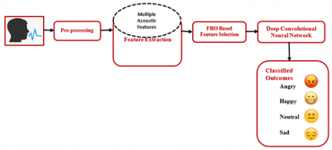
The framework of the proposed SER scheme is given in Figure 1 that encompasses the preprocessing, multiple acoustic feature extraction and DCNN for CCSER. The multiple acoustic features are used to capture the temporal variations in the emotion signal using time domain features, spectral properties of the signal using various spectral features and variation in amplitude and frequency of the voice signal using voice quality features. The DCNN improves the connectivity and correlation of the different local and global acoustic features for effective CCSER.
Table 2. Details about dataset used for CCSER
|
Dataset Details |
Hindi-IITKGP-SEHSC [45] |
Urdu [46] |
Telugu-IITKGP-SESC [43] |
Kannada [44] |
|
Language Family |
Indo-Aryan |
Indo-Aryan |
Dravidian |
Dravidian |
|
Languages |
Hindi |
Urdu |
Telugu |
Kannada |
|
No. of Emotions |
8 |
4 |
8 |
6 |
|
Emotion Classes |
Anger, Fear, Happy, Neutral, Sadness, Surprise, Disgust, Sarcastic |
Anger, Happy, Neutral, Sad |
Neutral, Anger, Happy, Compassion, Fear, Surprise, Disgust, Sarcastic |
Anger, Fear, Happy, Neutral, Sadness, Surprise |
|
Total No. of Samples |
1200 |
400 |
1200 |
468 |
|
No. of samples per Emotion |
150 |
100 |
150 |
78 |
|
No. of Speakers |
27 Male+ 11 Female |
27 Male+ 11 Female |
05 Male+ 05 Female |
04 Male+ 09 Female |
|
Recording Environment |
Controlled |
TV Talk shows |
Controlled |
Uncontrolled |
|
Total Duration |
|
|
7 Hours |
|
|
Availability |
Available on request |
Publicly available |
Available on request |
Publicly available |
Figure 1. Flow diagram of proposed system
3.3 Multiple acoustic features
Wide range of acoustic features are extracted for the signal to characterize the changes occurs in the voice due to emotion. The proposed feature set consists of time-domain features, spectral features and voice quality features as given in Table 3. The feature vector is further given to FH for prominent feature selection and these salient features are further given to DCNN architecture to improve the feature representation.
A. Multi-taper MFCC
Only one hamming window with a higher variance is used in generalized MFCC, which is unable to acquire the disparities over the frame of speech signal. The speech is filtered using moving average filter to lessen the amount of noise it contains during the pre-emphasis stage. As a part of framing process, the entire signal is divided into the frames of 40 ms each. This is necessary for multi-taper windowing to accumulate the adjoining spectral components together. The DFT is used to transform signals from the time to the spectral domain. The linearly scaled signal is then converted to Mel frequency, which can be perceived by human hearing. Discrete Cosine Transform (DCT) is used to transform signal back to time domain to reduce the signal's redundancies. 13 cepstral values are chosen as the features after log filter-bank energy has been calculated over the frames. Figure 2 depicts the MT-process MFCC's flow. In contrast, the windowing of the speech signal in the MT-MFCC uses various tappers with diverse variations, which aids in increasing frequency resolution.
Figure 2. MFCC coefficient extraction [7]
Table 3. Details regarding features
|
Types of Features |
Feature |
Size |
|
Time domain features |
Zero Crossing Rate (ZCR) |
1 |
|
Pitch Frequency (PF). |
1 |
|
|
Spectral domain |
Multi-taper Mel Frequency Coefficients (MTMFCCs), |
13 |
|
ΔMTMFCC Coefficients |
13 |
|
|
ΔΔ MTMFCC Coefficients |
13 |
|
|
Linear Predictive Cepstral Coefficients (LPCC) |
13 |
|
|
Spectral Kurtosis (SK) |
257 |
|
|
Formants |
3 |
|
|
Standard Deviation |
1 |
|
|
Mean of the Formants |
1 |
|
|
Voice quality |
Jitter |
1 |
|
Shimmer |
1 |
|
|
Total No. of Features |
318 |
|
The sign weighted ceptrum estimator (SWCE) provides low error compared with traditional MFCC as given in Eq. (1) [29, 30].
${{w}_{P}}\left( j \right)=\sqrt{\frac{2}{N+1}}\sin \left( \frac{\pi p\left( j+1 \right)}{N+1} \right),~j=0,1,\ldots ,N-1.$ (1)
where, N denotes total frames, $w_p$ depicts tapper window, and p=1,2,3, …., M.
The weights of SWCEfor each taper are estimated using Eq. (2) [31].
$\lambda \left( p \right)=\frac{\cos \left( \frac{2\pi \left( p-1 \right)}{M/2} \right)+1}{\mathop{\sum }_{p=1}^{M}\left( \cos \left( \frac{2\pi \left( p-1 \right)}{M/2} \right)+1 \right)},p=1,,2,\ldots ,M.$ (2)
where, M represent total tapers, $\lambda(\mathrm{p})$ denotes the weight of ${{p}^{th}}$ taper, and p =1,2,3, ……., M. The power spectral density (PSD) for different taper windows for speech signal is computed using Eq. (3) [29, 30].
${{\hat{S}}_{MT}}\left( m,k \right)=\underset{p=1}{\overset{M}{\mathop \sum }}\,\lambda \left( p \right){{\left| \underset{j=0}{\overset{N-1}{\mathop \sum }}\,{{w}_{P}}\left( j \right)s\left( m,j \right){{e}^{\frac{2\pi ik}{N}}} \right|}^{2}},$ (3)
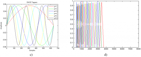
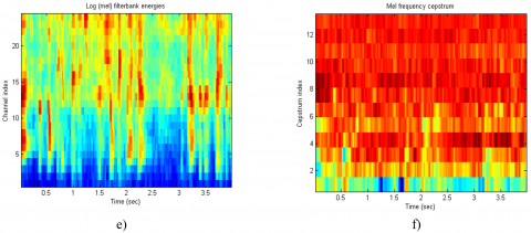
After multi-taper windowing the speech signal is converted in to spectral domain signal using fast Fourier transform (FFT). The Mel frequency spectrum is further changed in to time domain using DCT and to minimize the redundancy in the signal, Total 39 MTMFCC coefficients are considered for the representation of voice signal such as 13 MFCC coefficients, 13 $\Delta$-MTMFCC coefficients and 13 $\Delta$$\Delta$-MTMFCC coefficients. Figure 3 depicts the conception of the phases of MT-MFCC.
B. LPCC
The linear predictive analysis's spectral feature known as the LPCC is used to reflect the speech signal's emotion-specific phonological interpretation. The LPCC does a fantastic job of describing aspects of the human vocal tract that assist to specifically identify the emotional content of speech. In linear predictive analysis, the knowledge of prior p samples may be used to estimate the nth samples, as shown in Eq. (4).
$x\left( n \right)={{a}_{1}}x\left( n-1 \right)+{{a}_{2}}x\left( n-2 \right)+{{a}_{3}}x\left( n-3 \right)+~\ldots \ldots \ldots \ldots ~+~{{a}_{p}}x\left( n-p \right),$ (4)
where, $a_1, a_2, \ldots \ldots a_p$ are the constants over the speech frames. The speech sample is predicted by these linear predictor coefficients. The suggested method takes into account a total of 13 LPCC coefficients [13] as characteristics.
C. Spectral Kurtosis(SK)
This denotes the sequence of transients together with their spectral domain locations. It describes the non-Gaussianity or smoothness of the speech frequency spectrum around its centroid, which demonstrates the impact of varying levels of arousal and emotional valence on the speech spectrum. The spectral kurtosis of the voice is calculated using Eq. (5).
$SK=\frac{\mathop{\sum }_{k=b1}^{b2}{{\left( {{f}_{k}}-{{\mu }_{1}} \right)}^{4}}{{s}_{k}}}{{{\left( {{\mu }_{2}} \right)}^{4}}\mathop{\sum }_{k=b1}^{b2}{{s}_{k}}}$ (5)
Here, $\mu_1$ depicts the spectral centroid, $\mu_2$ denotes spectral spread respectively, ${{s}_{k}}$ is spectral value over $k$ bins, ${{b}_{1}}$ and ${{b}_{2}}$ are the lowest and highest bound of the bins where SK of voice is computed.
D. Formants
Formants are energetically intense frequency peaks in the spectrum. They are predominantly noticeable in vowels. Every formant has an associated vocal tract resonance that characterizes the influence of the emotion on the speech signal. Here, 3 formants, mean and standard deviation of formants are considered to characterize the spectral changes due to emotion in the voice signal.
E. Pitch Frequency
To illustrate the vocal component of communication, pitch $({{f}_{0}})$ is important. By calculating the disparity between the peaks obtained by the speech signal's autocorrelation, the pitch of the speech may be determined.
F. ZCR
ZCR offers the signal's passage through the zero line, which represents the degree of noise in the voice signal. ZCR is computed in the time domain via Equation 6. Over a time period, the sign function returns a value of ‘1’ for the positive amplitude and ‘0’ for negative amplitude (t) of speech.
$ZC{{R}_{t}}=\frac{1}{2}\left( \underset{n=1}{\overset{N}{\mathop \sum }}\,(sign\left( x\left[ n \right] \right)-sign(x\left[ n-1 \right] \right)$ (6)
G. Jitter and Shimmer
The fluctuations in frequency and amplitude of the speech induced by aperiodic vocal fold vibrations are known as jitter and shimmer, respectively. The breathiness, hoarseness and roughness of the emotional voice are portrayed by the jitter and shimmer. The mean jitter is given by Eq. (7).
$Jitter=\frac{1}{N-1}\underset{i=1}{\overset{N-1}{\mathop \sum }}\,\left| {{T}_{i}}-{{T}_{i+1}} \right|$ (7)
where,$~{{T}_{i}}$ denotes the time period in sec and $N$ provides total periods. Eq. (8) represents mean shimmer.
$Shimmer=\frac{\frac{1}{N-1}\mathop{\sum }_{i=1}^{N-1}\left| {{A}_{i}}-{{A}_{i+1}} \right|}{\frac{1}{N}\mathop{\sum }_{i=1}^{N}{{A}_{i}}},$ (8)
where, Ai is peak-to-peak amplitude of speech signal and N is the number of periods.
Eq. (9) represents the feature representation $\left( Feat \right)~$provided to FHO for selecting prominent feature.
$Feat=\left\{ MTMFC{{C}_{1-39}},~LPC{{C}_{1-13}},~Formant{{s}_{1-3}},~MeanForman{{t}_{1}},~StdForman{{t}_{1}},~~PitchFre{{q}_{1}},~ZC{{R}_{1}},~Jitte{{r}_{1}},~Shimme{{r}_{1}} \right\}$ (9)
Figure 3. Visualizations of MT-MFCC process a) Original speech Signal, b) Pre-emphasis effect, c) Multi-taper Windows (p=6), d) Mel filter bank, e) Mel log filterbank energy, f) Mel frequency cepstrum
3.4 FHO based feature selection
Finding significant features and reducing feature vector length both depend on feature selection. The SER system's output is enhanced by the less complex but still useful features. The FHO is a metaheuristic algorithm that mimics the fire hawk’s (FHs) fire-starting, fire-spreading, and prey-catching food foraging behaviour. To prevent local optimum entrapment, which improves global optimal solution, the FHO takes into account the average of the solution candidates in a certain region. Figure 4 shows the flow chart for effectively choosing characteristics from a collection of various acoustic features.
The biggest risks to animals and ecosystems come from wildfires that are caused by either a natural phenomenon or by humans. Many times, birds referred to as "fire hawks" such whistling kites, black kites, and brown falcons may purposely start a fire in order to catch prey to eat.
By holding the flaming sticks in its beak and dumping them over the area that hasn't yet caught fire, the fire hawk carefully spreads the flames in order to capture its victim. The fire hawks start little flames to frighten their prey, which includes snakes, rats, and other small animals. This causes the prey to make a hurried, panicked decision, which makes it easier for the FHs to capture the prey.
The number of viable solutions (A) shows where the FHs and their prey were first located. By taking into account the precise restrictions for each parameter as provided in (10) and (11), the population of FHs and preys is first initialized at random. Values of $\alpha, \beta$, and $K$ are taken into account by the populace. Here, N stands for the number of solutions, ${{A}_{ij}}$ signifies the ${{j}^{th}}$ decision variable of the ${{i}^{th}}$ solution, $\text{A}_{\text{i},\text{max}}^{\text{j}}$ and $\text{A}_{\text{i},\text{min}}^{\text{j}}$stands for the decision variable's upper and lower bounds, respectively.
$\begin{aligned} & A=\left[\begin{array}{c}A_1 \\ A_2 \\ A_3 \\ \vdots \\ A_N\end{array}\right]=\left[\begin{array}{ccc}A_{11} & A_{12} & A_{13} \\ A_{21} & A_{22} & A_{23} \\ A_{31} & A_{32} & A_{33} \\ \vdots & \vdots & \vdots \\ A_{N 1} & A_{N 2} & A_{N 3}\end{array}\right]=\left[\begin{array}{ccc}\alpha_{11} & \beta_{12} & K_{13} \\ \alpha_{21} & \beta_{22} & K_{23} \\ \alpha_{31} & \beta_{32} & K_{33} \\ \vdots & \vdots & \vdots \\ \alpha_{N 1} & \beta_{N 2} & K_{N 3}\end{array}\right]\end{aligned}$ (10)
Figure 4. FHO based feature selection strategy
$A_{i}^{j}\left( 0 \right)=A_{i,min}^{j}+rand.\left( A_{i,max}^{j}-A_{i,min}^{j} \right),\left\{ \begin{matrix} i=1,2,\ldots ,N. \\ j=1,2,\ldots ,d. \\ \end{matrix} \right.$ (11)
To assess the fitness of the solutions, the objective function based on the intra-class and inter-class variance is utilised. Other solutions are seen as prey while the ones with the best fitness are kept as FH. Global solutions are used to start fires since they are thought of as the original chief fires. To facilitate hunting, the chosen FHs are employed to start the fire in the unburned region. (12) and (13) include descriptions of the preys and FH. Here, $P{{R}_{m}}$ is ${{m}^{th}}$ prey in search space and $F{{H}_{n}}$ is ${{n}^{th}}$FH in search space.
$P R=\left[\begin{array}{c}P R_1 \\ P R_2 \\ P R_3 \\ \vdots \\ P R_m\end{array}\right]$ (12)
$F H=\left[\begin{array}{c}F H_1 \\ F H_1 \\ F H_1 \\ \vdots \\ F H_n\end{array}\right]$ (13)
In next phase, the FH catches the nearby prey based on distance metrics given in 14. Here, $D_{k}^{l}$ shows distance between ${{l}^{th}}$FH and ${{k}^{th}}$ prey, $\left( {{x}_{1}},{{y}_{1}} \right)$ and $\left( {{x}_{2}},{{y}_{2}} \right)$indicates the coordinates of location of FH and prey.
$D_k^l=\sqrt{\left(x_2-x_1\right)^2+\left(y_2-y_1\right)^2},\left\{\begin{array}{l}l=1,2, \ldots, n \\ k=1,2, \ldots, m\end{array}\right.$ (14)
The FHs choose burning sticks and start fires in unburned areas of their territory during the next phase to trap their prey and make their escape fast and challenging. The FHs use (15) to update their location in order to defend their area and stop other fire hawks from grabbing burning sticks. In this case, the values of ${{r}_{1}}$ and ${{r}_{2}}$ are arbitrary numbers between 0 and 1 that control the direction of the FHs raids on the main fire (global solution).
$\text{FH}_{\text{l}}^{\text{new}}=\text{F}{{\text{H}}_{1}}+\left( {{\text{r}}_{1}}\times \text{GB}-{{\text{r}}_{2}}\times \text{F}{{\text{H}}_{\text{Near}}} \right),\text{ }\!\!~\!\!\text{ l}=1,2,\ldots ,\text{n}.$ (15)
When the prey sees the flaming sticks laid out on the ground, it begins to flee, hide, or inadvertently run towards the hawks. Using (16), the prey's location is updated for this case. Here, ${{r}_{3}}$ and ${{r}_{5}}$ are random numbers between [0,1] which represent coefficients for the movement towards hawks and a safe spot, and $\text{PR}_{\text{q}}^{\text{new}}$ represents the prey encircled by lthfire hawks.
$\begin{aligned} & \mathrm{PR}_{\mathrm{q}}^{\text {new }}=\mathrm{PR}_{\mathrm{q}}+\left(\mathrm{r}_3 \times \mathrm{FH}_1\right. \left.-r_4 \times S P_1\right),\left\{\begin{array}{l}l=1,2, \ldots, n. \\ q=1,2, \ldots, r.\end{array}\right. \\ & \end{aligned}$ (16)
The prey may sometimes relocate to another hawk's territory or to the safest location outside the area. The updated position is shown by the number (17). Here,$~{{r}_{5}}$and ${{r}_{6}}$stand for the random number between [0, 1] that designates the coefficients for the migration of prey towards other hawks and towards safe locations beyond the region.
$\begin{aligned} & \mathrm{PR}_{\mathrm{q}}^{\text {new }}=\mathrm{PR}_{\mathrm{q}}+\left(\mathrm{r}_5 \times \mathrm{FH}_{\text {Alter }}\right.\left.-r_6 \times \text{SP}\right),\left\{\begin{array}{l}l=1,2, \ldots, n. \\ q=1,2, \ldots, r.\end{array}\right. \\ & \end{aligned}$ (17)
The safest region where all animals assemble together for shelter which is given by (18) and (19) where $\text{P}{{\text{R}}_{\text{q}}}$ is $q$th prey encircled by $l$th FH.
$\text{S}{{\text{P}}_{1}}=\frac{\mathop{\sum }_{\text{q}=1}^{\text{r}}\text{P}{{\text{R}}_{\text{q}}}}{\text{r}},\left\{ \begin{matrix}q=1,2,\ldots ,r. \\ l=1,2,\ldots ,n. \\ \end{matrix} \right.$ (18)
$\text{SP}=\frac{\mathop{\sum }_{\text{k}=1}^{\text{m}}\text{P}{{\text{R}}_{\text{k}}}}{\text{m}},\text{k}=1,2,\ldots ,\text{m}.$ (19)
The fitness of the solution is calculated using (20) which is based on the intra-class and inter-class variability of the speech features. The higher inter-class and lower intra-class feature variability helps to selects the hugely discriminative combination of feature set for SER.
$Fitnes{{s}_{F{{H}_{i}}}}=\frac{{{\text{ }\!\!\sigma\!\!\text{ }}_{\text{inter}-\text{class}}}}{{{\text{ }\!\!\sigma\!\!\text{ }}_{\text{intra}-\text{class}}}}$ (20)
3.5 DCNN architecture
The DCNN provides the short term and long-term correlation and connectivity in the local and global features extracted using MAF. It characterizes the changes occurs on the valence and arousal on the voice due to emotion. It helps to represent the variations in intonation, prosody and timbre of the speech because of the emotions and language. It provides high level abstract features that give better distinctiveness for different emotions. The proposed lightweight DCNN consist of three layers of sequential CNN. Each layer of CNN consists of convolution layer (Conv), Rectified Linear Unit Layer (ReLU), and maximum pooling layer (MaxPool). The DCNN accepts the handcrafted feature vector that represents various spectral, temporal and voice quality features of the emotion signal. The first layer in proposed DCNN includes three layers {Conv1(KernelSize-1×3, NumFilter-64, Stride-1, ZeroPadding-Yes) →ReLU1 (Stride-1) →MaxPool1 (Stride-2)} which accepts multiple acoustic feature vector as an input with dimensions of (1×318) and produces the output feature map of (1×318×64). Zero padding maintains the original dimensions of the multiple acoustic features. The second layer is made up of {Conv2(KernelSize-1×3, NumFilter-128, Stride-1, ZeroPadding-Yes) →ReLU2(Stride-1) →MaxPool2(Stride-2)}. Third layer encompasses {Conv3(KernelSize-1×3, NumFilter-256, Stride-1, ZeroPadding-Yes) →ReLU3 (Stride-1) →MaxPool2(Stride-2)}.
The convolution layer feature map $y\left( n \right)$ of 1-D acoustic features A$\left( n \right)$ and L convolution filter $k\left( n \right)$using Eq. (21). Eq. (22) describes convolution feature map where $\text{y}_{\text{i}}^{\text{l}}$ stands for ith feature map of ${{l}^{th}}$ layer, $\text{y}_{\text{j}}^{\text{l}-1}$ denotesjth feature of ${{\left( l-1 \right)}^{th}}$ layer, $\text{k}_{\text{ij}}^{\text{l}}$ representthe filter kernel of ${{l}^{th}}$ layer linked to $j$ feature, $\text{b}_{\text{i}}^{\text{l}}$ denotes for bias and $\text{ }\!\!\sigma\!\!\text{ }$ symbolizesReLU activation function. The ReLU activation function is faster and simple that replaces negative values by 0 to overcome the vanishing gradient issue using Eq. (23).
$y\left( n \right)=A\left( n \right)\times k\left( n \right)=\underset{m=0}{\overset{L-1}{\mathop \sum }}\,A\left( m \right).k\left( n-m \right)$ (21)
$y_{i}^{l}=\sigma \left( b_{i}^{l}+\underset{j}{\mathop \sum }\,y_{j}^{l-1}\times k_{ij}^{l} \right)$ (22)
$\sigma \left( y \right)=\max \left( 0,y \right)$ (23)
Subsequent to three CNN layers, a FC layers is used having 4 hidden layers. Lastly, Softmax classifier offers the likelihood of the output class where utmost class label probability results in output class label using Eqs. (24)-(26). The Softmax classifier selected for the SER classification as it is simple probabilistic classifier which is simple, needs less computation compared with traditional classifiers and helps to minimize computational burden on the system.
${{z}_{i}}=\underset{j}{\mathop \sum }\,{{h}_{j}}{{w}_{ji}}$ (24)
${{p}_{i}}=\frac{\text{exp}\left( {{z}_{i}} \right)}{\mathop{\sum }_{j=1}^{n}\text{exp}\left( {{z}_{j}} \right)}$ (25)
$\hat{y}=arg\begin{matrix} max \\ i \\\end{matrix}{{p}_{i}}$ (26)
Here, hj denotes penultimate layer's weight, ${{\text{w}}_{\text{ji}}}$describes the weights joining Softmax and penultimate layer, ${{\text{z}}_{\text{i}}}$ representsSoftmax layer input, ${{\text{p}}_{\text{i}}}$stands for class label probability and $\hat{y}$ indicates label of predicted class. The outcome of proposed DCNN is estimated mini-batch gradient descent optimization (MBGD) learning algorithm. In MBGD algorithm n complete dataset is divided in to small batches b, then the model weights are reorganized utilizing model error given in Eq. (27).
${{E}_{t}}[f\left( w \right)=\frac{1}{b}\underset{k=\left( t-1 \right)b+1}{\overset{tb}{\mathop \sum }}\,f\left( w,{{T}_{i}} \right)$ (27)
The weights are updated using Eq. (28).
${{w}^{t+1}}={{w}^{t}}-\mu {{\nabla }_{w}}{{E}_{t}}\left[ f\left( {{w}^{t}} \right) \right]$ (28)
where, $E_t$ provides model error, $T_i$ stands for training samples, $W$ denotes weights of filter kernel, $F$ provides cost function, $\mu$ shows learning rate, $\nabla$ describes gradient of cost function and $t_b$ provides number of batches.
The anticipated SER scheme is implemented using MATLAB 2019b on the personal computer with 16GB RAM and core i7 processor on Windows environment.
4.1 Parameter configurations
The parameter configurations and initial hyper-parameters for the DCNN architecture are summarized in Table 4 and Table 5 respectively. The FHO selects 200 features with higher inter-class and lower intra-class variance which are provided to the DCNN foe emotion recognition. Table 4 describes the input size for every layer, filter size, number of filters, stride value, padding, output activations and total trainable parameters of the DCNN. The proposed DCNN requires 149120 trainable parameters which lead to the lower training time (17.20min). However, the proposed model needs 163460 trainable parameters when all features are fed to DCNN.
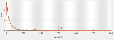
Figures 5 and 6 depict the training outcome and loss of the proposed DCNN for MBGD algorithm 6 respectively. The MBGDM algorithm is preferred over the ADAM, SGDM and RMSPropalgorithm because it is faster, reliable, robust for the variable data, provides better generalization during error updation, and minimizes the training duration by splitting the training data in the batch size of 64. The moderate learning rate of 0.01 is selected to avoid under-fitting and over-fitting.
Table 4. Parameter specification of proposed DCNN
|
Layer |
Sub-layer |
Input Size |
Filter Size |
No of Filters |
Stride |
Padding |
Output Feature Map |
Total Trainable Parameters |
|
Input |
- |
1×200 |
- |
- |
- |
- |
1×200 |
- |
|
CNN1 |
Conv1 |
1×200×64 |
1×3 |
64 |
1 |
2 |
1×200×64 |
256 |
|
ReLU1 |
1×200×64 |
- |
- |
1 |
- |
1×200×64 |
- |
|
|
MaxPool1 |
1×100×64 |
- |
- |
2 |
- |
1×100×64 |
- |
|
|
CNN2 |
Conv2 |
1×100×128 |
1×3 |
128 |
1 |
2 |
1×100×128 |
24704 |
|
ReLU2 |
1×100×128 |
- |
- |
1 |
- |
1×100×128 |
- |
|
|
MaxPool2 |
1×50×128 |
|
|
2 |
|
1×50×128 |
|
|
|
CNN3 |
Conv3 |
1×50×128 |
1×3 |
256 |
1 |
2 |
1×50×256 |
98560 |
|
ReLU3 |
1×50×256 |
- |
- |
1 |
- |
1×50×256 |
- |
|
|
MaxPool3 |
1×25×256 |
|
|
2 |
|
1×25×256 |
|
|
|
FC Layer |
- |
1×4 |
- |
- |
- |
- |
1×4 |
25600 |
|
Classification Layer |
- |
1×4 |
- |
- |
- |
- |
4×1 |
- |
|
Total trainable Parameters |
149120 |
|||||||
Table 5. CNN implementation initial parameters
|
Parameter |
Specification |
|
Mini Batch Size |
64 |
|
Maximum Epoch |
50 |
|
L2 Regulation |
10^4 |
|
Initial Learning Rate |
0.01 |
|
Initial Bias |
1 |
|
Gradient Threshold Method |
L2 Norm |
|
Gradient Threshold |
Inf |
Figure 5. Training accuracy of proposed model
Figure 6. Training loss of proposed model
4.2 Evaluation metrics
The outcome of suggested CCSER is estimated using various qualitative and quantitative outcome metrics. The precision and recall provide the qualitative and quantitative measure respectively of the proposed CCSER for different training and testing scenario. Accuracy gives the overall recognition rate and F1-score provides the balance between precision and recall. The precision, recall, accuracy and F1-score are computed using Eqs. (29)-(32). Here, TP, TN, FP and FN represent true positive, true negative, false positive and false negative rates of the recognition result.
$Precision=\frac{TP}{TP+FP}$ (29)
$Recall=\frac{TP}{TP+FN}$ (30)
$Accuracy~=\frac{TP+TN}{TP+TN+FP+FN}\times 100$ (31)
$F1-score=\frac{2\times Precision\times Recall}{Precision+Recall}$ (32)
4.3 FHO based feature selection
The FHO is employed for the different population ranging from 10 to 318. The FHO provides higher inter-class and lower intra-class variability for the 200 features selected from the multiple acoustic features. The behavior of the inter-class and intra-class variability of the features obtained using FHO algorithm is represented in Figure 7. It is observed that MFCC. Jitter, shimmer, ZCR, PF and some spectral kurtosis features always ranks in features which shows higher influence of emotion.
Figure 7. Inter-class and intra-class variance of the features
4.4 SER results and discussions
The outcome of the proposed multiple acoustic features (200 features selected using FHO) and DCNN is evaluated for the single corpus SER where same corpus data is used for the training and testing. Table 6 shows that the offered scheme provides better results for the single corpus SER. It results in an accuracy of 90.52%,84.00%, 90.60% and 89.00%, for the four Indian corpus such as Hindi, Urdu, Telugu and Kannada, respectively. It is observed that for the Indo-Aryan and Dravidian corpuses the single corpus SER recognition shows less variance.
Table 6. Outcome of proposed system for single corpus SER
|
Train Dataset |
Test Dataset |
Accuracy |
Precision |
Recall |
F1-score |
|
Hindi |
Hindi |
90.52 |
0.91 |
0.90 |
0.90 |
|
Urdu |
Urdu |
84.00 |
0.85 |
0.84 |
0.85 |
|
Telugu |
Telugu |
90.60 |
0.88 |
0.90 |
0.89 |
|
Kannada |
Kannada |
89.00 |
0.89 |
0.89 |
0.89 |
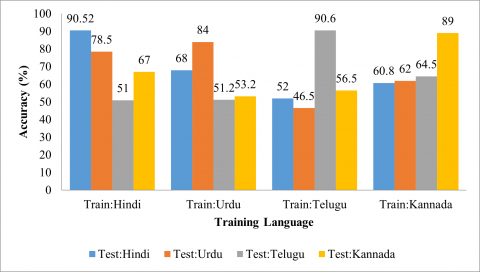
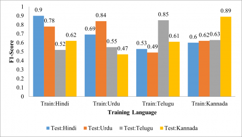
The cross-corpus SER evaluations are considered by training the proposed system for one corpus and testing another corpus on the system. Figures 8-11 show the accuracy, precision, recall and F1-Scorerespectively for the cross corpus SER for Hindi, Urdu, Telugu and Kannada language. When the system is trained for Hindi language and other Urdu, Telugu and Kannada are used for testing purpose then the system provides 78.50%, 51.00% and 67.00% accuracy for Urdu, Telugu and Kannada respectively. The proposed scheme shows higher accuracy for Hindi language (68.00%) when the system is trained for Urdu Language. It is observed that when Indo-Aryan languages are used for the training purpose then other Indo-Aryan give significantly better outcome compared with Dravidian languages. Also, when the system is trained for Kannada corpus then Telugu Corpus (64.00%) provides better accuracy compared with other corpuses such as Hindi (60.82%) and Urdu (62.00%). Similarly, when the system is trained for Telugu corpus then Kannada Corpus (56.50%) provides better accuracy compared with other corpuses such as Hindi (52.00%) and Urdu (46.50%). The vast changes in syllable, intonation, prosodic parameters and pitch of speech lead to the deviation in cross-corpus SER rate.
Figure 8. Accuracy for proposed method for CCSER
Figure 9. Precision for proposed method for CCSER
Figure 10. Recall for proposed method for CCSER
Figure 11. F1-Score for proposed method for CCSER
Table 7. Outcome evaluation of proposed system for multilingual training
|
Train Dataset |
Test Dataset |
Accuracy |
Precision |
Recall |
F1-score |
|
Hindi+ Kannada+ Urdu+ Telugu |
Hindi |
58.83 |
0.64 |
0.58 |
0.58 |
|
Urdu |
61.75 |
0.66 |
0.61 |
0.56 |
|
|
Telugu |
69.75 |
0.69 |
0.69 |
0.69 |
|
|
Kannada |
45.51 |
0.50 |
0.45 |
0.44 |
The usefulness of the proposed CCSER is assessed for the multi-corpus training as described in the Table 7. For the multi-corpus training all four languages 70% samples are used for the training and individual language is tested on the trained model independently. When the corpuses are nixed together it decreases the distinctiveness of the particular corpus due language variability. The multi-corpus training results in 58.83%, 61.75%, 69.75% and 45.51% accuracy for the Hindi, Urdu, Telugu and Kannada languages respectively. It is observed that the multi-lingual training needs language adaptation to conquer the linguistic, regional and intonation variations in Indian corpuses.
The proposed system can be collaborated with the different HMI and social networking sites to understand and analyze the emotions using Indian languages. The systems can be useful for emotion annotating the movies and web series of unknown language of the user. The system has shown significant achievement for the CCSER but its performance is limited due to less dataset, larger time, and variance in regional languages in Indian corpuses.
This paper presents cross-corpus SER using multiple acoustic features and one dimensional DCNN. The outcome of proposed CCSER is evaluated on the four Indian dataset such as Hindi, Urdu, Telugu and Kannada using the performance metrics such as accuracy, precision, recall and F1-score. It provides an accuracy of 58.83%, 61.75%, 69.75% and 45.51% for Hindi, Urdu, Telugu and Kannada language respectively for multi-lingual training. The FHO based feature selection strategy provides the efficient selection of prominent features and helps to get better SER accuracy and minimize the trainable parameters. The proposed DCNN assists to boost the distinctiveness of the low-level features of voice signal. The DCNN integrates global and local features, enhancing the differentiation between emotions and promoting generalization in SER.It is found that the proposed FHO-based multiple acoustic features selection assist to increase the outcome of the CCSER that considers raw speech as the input and spectrogram as the input. The proposed CCSER system helps to improve the generalization capability of the traditional SER systems.It enhances the emotional assistance to the user interacting with person/client on online platform.In future, the outcomes of suggested DCNN based SER can be improved using domain adaptation and more global and local acoustic features.
[1] Abbaschian, B.J., Sierra-Sosa, D., Elmaghraby, A. (2021). Deep learning techniques for speech emotion recognition, from databases to models. Sensors, 21(4): 1249. https://doi.org/10.3390/s21041249
[2] Wani, T.M., Gunawan, T.S., Qadri, S.A.A., Kartiwi, M., Ambikairajah, E. (2021). A comprehensive review of speech emotion recognition systems. IEEE Access, 9: 47795-47814. https://doi.org/10.1109/ACCESS.2021.3068045
[3] Kawade, R., Bhalke, D.G. (2022). Speech emotion recognition based on wavelet packet coefficients. In: Kumar, A., Mozar, S. (eds) ICCCE 2021. Lecture Notes in Electrical Engineering, vol 828. Springer, Singapore. https://doi.org/10.1007/978-981-16-7985-8_86
[4] Fahad, M.S., Ranjan, A., Yadav, J., Deepak, A. (2021). A survey of speech emotion recognition in natural environment. Digital Signal Processing, 110: 102951. https://doi.org/10.1016/j.dsp.2020.102951
[5] Kawade, R., Konade, R., Majukar, P., Patil, S. (2022). Speech emotion recognition using 1D CNN-LSTM network on Indo-Aryan database. In 2022 Third International Conference on Intelligent Computing Instrumentation and Control Technologies (ICICICT), Kannur, India, pp. 1288-1293. https://doi.org/10.1109/ICICICT54557.2022.9917635
[6] Bhangale, K.B., Titare, P., Pawar, R., Bhavsar, S. (2018). Synthetic speech spoofing detection using MFCC and radial basis function SVM. IOSR Journal of Engineering (IOSRJEN), 8(6): 55-62.
[7] Bhangale, K., Kothandaraman, M. (2023). Speech emotion recognition based on multiple acoustic features and deep convolutional neural network. Electronics, 12(4): 839. https://doi.org/10.3390/electronics12040839
[8] Bhangale, K.B., Kothandaraman, M. (2023). Speech emotion recognition using the novel PEmoNet (Parallel Emotion Network). Applied Acoustics, 212: 109613. https://doi.org/10.1016/j.apacoust.2023.109613
[9] Bhangale, K.B., Mohanaprasad, K. (2021). A review on speech processing using machine learning paradigm. International Journal of Speech Technology, 24: 367-388. https://doi.org/10.1007/s10772-021-09808-0
[10] Jahangir, R., Teh, Y.W., Hanif, F., Mujtaba, G. (2021). Deep learning approaches for speech emotion recognition: State of the art and research challenges. Multimedia Tools and Applications, 80: 23745-23812. https://doi.org/10.1007/s11042-020-09874-7
[11] Thakur, A., Dhull, S. (2021). Speech emotion recognition: A review. In: Hura, G.S., Singh, A.K., Siong Hoe, L. (eds) Advances in Communication and Computational Technology. ICACCT 2019. Lecture Notes in Electrical Engineering, 668. https://doi.org/10.1007/978-981-15-5341-7_61
[12] Bhangale, K., Mohanaprasad, K. (2022). Speech emotion recognition using mel frequency log spectrogram and deep convolutional neural network. In: Sivasubramanian, A., Shastry, P.N., Hong, P.C. (eds) Futuristic Communication and Network Technologies. VICFCNT 2020. Lecture Notes in Electrical Engineering, vol 792. Springer, Singapore. https://doi.org/10.1007/978-981-16-4625-6_24
[13] Shahin, I., Nassif, A.B., Hamsa, S. (2019). Emotion recognition using hybrid Gaussian mixture model and deep neural network. IEEE Access, 7: 26777-26787. https://doi.org/10.1109/ACCESS.2019.2901352
[14] Mao, S., Tao, D., Zhang, G., Ching, P.C., Lee, T. (2019). Revisiting hidden Markov models for speech emotion recognition. In ICASSP 2019-2019 IEEE International Conference on Acoustics, Speech and Signal Processing (ICASSP), Brighton, UK, pp. 6715-6719. https://doi.org/10.1109/ICASSP.2019.8683172
[15] Kerkeni, L., Serrestou, Y., Raoof, K., Mbarki, M., Mahjoub, M.A., Cleder, C. (2019). Automatic speech emotion recognition using an optimal combination of features based on EMD-TKEO. Speech Communication, 114: 22-35. https://doi.org/10.1016/j.specom.2019.09.002
[16] Umamaheswari, J., Akila, A. (2019). An enhanced human speech emotion recognition using hybrid of PRNN and KNN. In 2019 International Conference on Machine Learning, Big Data, Cloud and Parallel Computing (COMITCon), Faridabad, India, pp. 177-183. https://doi.org/10.1109/COMITCon.2019.8862221
[17] Chen, L., Su, W., Feng, Y., Wu, M., She, J., Hirota, K. (2020). Two-layer fuzzy multiple random forest for speech emotion recognition in human-robot interaction. Information Sciences, 509: 150-163. https://doi.org/10.1016/j.ins.2019.09.005
[18] Akçay, M.B., Oğuz, K. (2020). Speech emotion recognition: Emotional models, databases, features, preprocessing methods, supporting modalities, and classifiers. Speech Communication, 116: 56-76. https://doi.org/10.1016/j.specom.2019.12.001
[19] Wei, P., Zhao, Y. (2019). A novel speech emotion recognition algorithm based on wavelet kernel sparse classifier in stacked deep auto-encoder model. Personal and Ubiquitous Computing, 23: 521-529. https://doi.org/10.1007/s00779-019-01246-9
[20] Issa, D., Demirci, M.F., Yazici, A. (2020). Speech emotion recognition with deep convolutional neural networks. Biomedical Signal Processing and Control, 59: 101894. https://doi.org/10.1016/j.bspc.2020.101894
[21] Liu, D., Chen, L., Wang, Z., Diao, G. (2021). Speech expression multimodal emotion recognition based on deep belief network. Journal of Grid Computing, 19(2): 22. https://doi.org/10.1007/s10723-021-09564-0
[22] Zhang, S., Zhao, X., Tian, Q. (2019). Spontaneous speech emotion recognition using multiscale deep convolutional LSTM. IEEE Transactions on Affective Computing, 13(2): 680-688. https://doi.org/10.1109/TAFFC.2019.2947464
[23] Chen, M., He, X., Yang, J., Zhang, H. (2018). 3-D convolutional recurrent neural networks with attention model for speech emotion recognition. IEEE Signal Processing Letters, 25(10): 1440-1444. https://doi.org/10.1109/LSP.2018.2860246
[24] Bhangale, K.B., Kothandaraman, M. (2022). Survey of deep learning paradigms for speech processing. Wireless Personal Communications, 125(2): 1913-1949. https://doi.org/10.1007/s11277-022-09640-y
[25] Yao, Z., Wang, Z., Liu, W., Liu, Y., Pan, J. (2020). Speech emotion recognition using fusion of three multi-task learning-based classifiers: HSF-DNN, MS-CNN and LLD-RNN. Speech Communication, 120: 11-19. https://doi.org/10.1016/j.specom.2020.03.005
[26] Zhang, S., Zhang, S., Huang, T., Gao, W. (2017). Speech emotion recognition using deep convolutional neural network and discriminant temporal pyramid matching. IEEE Transactions on Multimedia, 20(6): 1576-1590. https://doi.org/10.1109/TMM.2017.2766843
[27] Neumann, M. (2018). Cross-lingual and multilingual speech emotion recognition on English and French. In 2018 IEEE International Conference on Acoustics, Speech and Signal Processing (ICASSP), Calgary, AB, Canada, pp. 5769-5773. https://doi.org/10.1109/ICASSP.2018.8462162
[28] Zhao, J., Mao, X., Chen, L. (2018). Learning deep features to recognise speech emotion using merged deep CNN. IET Signal Processing, 12(6): 713-721. https://doi.org/10.1049/iet-spr.2017.0320
[29] Ocquaye, E.N.N., Mao, Q., Song, H., Xu, G., Xue, Y. (2019). Dual exclusive attentive transfer for unsupervised deep convolutional domain adaptation in speech emotion recognition. IEEE Access, 7: 93847-93857. https://doi.org/10.1109/ACCESS.2019.2924597
[30] Lotfian, R., Busso, C. (2019). Curriculum learning for speech emotion recognition from crowdsourced labels. IEEE/ACM Transactions on Audio, Speech, and Language Processing, 27(4): 815-826. https://doi.org/10.1109/TASLP.2019.2898816
[31] Tripathi, S., Kumar, A., Ramesh, A., Singh, C., Yenigalla, P. (2019). Deep learning based emotion recognition system using speech features and transcriptions. arXiv preprint arXiv:1906.05681. https://doi.org/10.48550/arXiv.1906.05681
[32] Zhao, J., Mao, X., Chen, L. (2019). Speech emotion recognition using deep 1D & 2D CNN LSTM networks. Biomedical signal processing and control, 47: 312-323. https://doi.org/10.1016/j.bspc.2018.08.035
[33] Peng, Z., Li, X., Zhu, Z., Unoki, M., Dang, J., Akagi, M. (2020). Speech emotion recognition using 3d convolutions and attention-based sliding recurrent networks with auditory front-ends. IEEE Access, 8: 16560-16572. https://doi.org/10.1109/ACCESS.2020.2967791
[34] Xiao, Y., Zhao, H., Li, T. (2020). Learning class-aligned and generalized domain-invariant representations for speech emotion recognition. IEEE Transactions on Emerging Topics in Computational Intelligence, 4(4): 480-489. https://doi.org/10.1109/TETCI.2020.2972926
[35] Ai, X., Sheng, V.S., Fang, W., Ling, C.X., Li, C. (2020). Ensemble learning with attention-integrated convolutional recurrent neural network for imbalanced speech emotion recognition. IEEE Access, 8: 199909-199919. https://doi.org/10.1109/ACCESS.2020.3035910
[36] Xia, X., Jiang, D., Sahli, H. (2020). Learning salient segments for speech emotion recognition using attentive temporal pooling. IEEE Access, 8: 151740-151752. https://doi.org/10.1109/ACCESS.2020.3014733
[37] Chen, G., Zhang, S., Tao, X., Zhao, X. (2020). Speech emotion recognition by combining a unified first-order attention network with data balance. IEEE Access, 8: 215851-215862. https://doi.org/10.1109/ACCESS.2020.3038493
[38] Zhao, H., Xiao, Y., Zhang, Z. (2020). Robust semisupervised generative adversarial networks for speech emotion recognition via distribution smoothness. IEEE Access, 8: 106889-106900. https://doi.org/10.1109/ACCESS.2020.3000751
[39] Falahzadeh, M.R., Farokhi, F., Harimi, A., Sabbaghi-Nadooshan, R. (2023). Deep convolutional neural network and gray wolf optimization algorithm for speech emotion recognition. Circuits, Systems, and Signal Processing, 42(1): 449-492. https://doi.org/10.1007/s00034-022-02130-3
[40] Prakash, P.R., Anuradha, D., Iqbal, J., Galety, M.G., Singh, R., Neelakandan, S. (2023). A novel convolutional neural network with gated recurrent unit for automated speech emotion recognition and classification. Journal of Control and Decision, 10(1): 54-63. https://doi.org/10.1080/23307706.2022.2085198
[41] Aggarwal, A., Srivastava, A., Agarwal, A., Chahal, N., Singh, D., Alnuaim, A.A., Alhadlaq A,Lee, H.N. (2022). Two-way feature extraction for speech emotion recognition using deep learning. Sensors, 22(6): 2378. https://doi.org/10.3390/s22062378
[42] Song, P. (2017). Transfer linear subspace learning for cross-corpus speech emotion recognition. IEEE Transactions on Affective Computing, 10(2): 265-275. https://doi.org/10.1109/TAFFC.2017.2705696
[43] Koolagudi, S.G., Maity, S., Kumar, V.A., Chakrabarti, S., Rao, K.S. (2009). IITKGP-SESC: Speech database for emotion analysis. In: Ranka, S., et al. Contemporary Computing. IC3 2009. Communications in Computer and Information Science, vol 40. Springer, Berlin, Heidelberg. https://doi.org/10.1007/978-3-642-03547-0_46
[44] Agrawal, V. (2022). A Kannada Emotional Speech Dataset Zenodo. https://doi.org/10.5281/zenodo.6345107
[45] Koolagudi, S.G., Reddy, R., Yadav, J., Rao, K.S. (2011). IITKGP-SEHSC: Hindi speech corpus for emotion analysis. In 2011 International conference on devices and communications (ICDeCom), Mesra, India, pp. 1-5. https://doi.org/10.1109/ICDECOM.2011.5738540
[46] Latif, S., Qayyum, A., Usman, M., Qadir, J. (2018). Cross lingual speech emotion recognition: Urdu vs. western languages. In 2018 International Conference on Frontiers of Information Technology (FIT), Islamabad, Pakistan, pp. 88-93. https://doi.org/10.1109/FIT.2018.00023
[47] Gupta, N., Thakur, V., Patil, V., Vishnoi, T., Bhangale, K. (2023). Analysis of affective computing for marathi corpus using deep learning. In 2023 4th International Conference for Emerging Technology (INCET), Belgaum, India, pp. 1-8. https://doi.org/10.1109/INCET57972.2023.10170346
[48] Bhangale, K., Dhake, D., Kawade, R., Dhamale, T., Patil, V., Gupta, N., Thakur, V., Vishnoi, T. (2023). Deep learning-based analysis of affective computing for Marathi corpus. In 2023 3rd International Conference on Intelligent Technologies (CONIT), Hubli, India, pp. 1-6. https://doi.org/10.1109/CONIT59222.2023.10205770
[49] Appidi, A.R., Srirangam, V.K., Suhas, D., Shrivastava, M. (2020). Creation of corpus and analysis in code-mixed Kannada-English twitter data for emotion prediction. In Proceedings of the 28th International Conference on Computational Linguistics, pp. 6703-6709. https://doi.org/10.18653/v1/2020.coling-main.587
[50] Garg, K., Lobiyal, D.K. (2020). Hindi EmotionNet: A scalable emotion lexicon for sentiment classification of Hindi text. ACM Transactions on Asian and Low-Resource Language Information Processing (TALLIP), 19(4): 1-35. https://doi.org/10.1145/3383330