Ahlem Chalabi*![]() | Safia Nait-Bahloul
| Safia Nait-Bahloul![]()
© 2024 The authors. This article is published by IIETA and is licensed under the CC BY 4.0 license (http://creativecommons.org/licenses/by/4.0/).
OPEN ACCESS
Association rules mining is one of the most relevant techniques in data mining. Aimed at identifying interesting connections and associations among groups of items or products within extensive transactional databases. However, this technique can yield too many rules, among which some are irrelevant and/or redundant. Thus, may present obstacles for the decision-maker. This Highlights the importance and challenge of evaluating extracted knowledge to define the most interesting association rules. In order to address this issue, we presented a constraint programming approach to evaluate the relevance of association rules. Our MeAR-CP approach involves filtering association rules using metrics such as IR, Cosine, Lift, Kulc as constraints solved by Choco constrain programming tools, and proposed our metric called 'Score'. The experiments are conducted on various datasets from the UCI Machine Learning Repository. We evaluate both time and rules. The results obtained from our experiments underscore the effectiveness of our approach in reducing irrelevant and redundant rules within an effective timeframe.
association rules, constraint programming, datamining, evaluation of association rules, metrics
Today the data collected is stored in diverse databases, where each record holds numerous attributes, totaling millions of records. Therefore, it is necessary to develop effective tools to explore this abundant information in order to extract useful knowledge.
Data Mining is a computer science discipline aimed at extracting rules to explain certain relationships between data or to plan actions in the future. Association rules are one of the most used techniques in the data mining process used in different fields like market basket problem, help decision maker, prediction, traffic Accidents [1], E-Commerce [2]. This technique is of great interest to the community where several researches have been carried out in order to develop new algorithms.
Typically, in the rule extraction process, two metrics are used: support and confidence. Very often, this technique leads to obtain too many rules that are not all necessarily relevant or sometimes even redundant [3]. Certainly, there may be intriguing rules with low frequency and obvious rules with high frequency. Moreover, the rules obtained might be very similar. In other words, they could describe either the same transactions or the same items [4]. This is contrary to the principle of Occam's Razor or the principle of simplicity, which states that the explanation requiring the fewest assumptions should be favored.
Despite the sophistication of modern data mining algorithms, the presence of irrelevant rules can obscure meaningful insights, increase computational complexity, and diminish the utility of the extracted knowledge. To illustrate this problem, we utilize an example presented in Table 1.
Table 1. Table of association rules
|
Rules |
Antecedent |
Consequent |
|
1 |
coffee |
milk |
|
2 |
coffee |
sugar |
|
3 |
coffee |
milk, sugar |
|
4 |
milk |
sugar |
|
5 |
milk |
cereal |
|
6 |
milk |
cereal, sugar |
For example, the rules (1, 2, 4 and 5) in Table 1 are redundant. Indeed, rules 1 and 2 as well as rules 4 and 5 are redundant with rules 3 and 6 respectively. If we want to determine the ratio of irrelevance for this example, we use the formula: Ratio of irrelevant rules=(Number of irrelevant rules/Total number of rules examined) * 100%. Ratio of irrelevant rules=(4/6) * 100%=66.66%. This shows that the majority of rules are irrelevant, potentially leading to higher memory and time usage in the process. Furthermore, these irrelevant rules may present obstacles for decision-makers.
It is therefore possible to eliminate rules 1, 2, 4 and 5 without losing knowledge, thus reducing extraction process time. This is why support and confidence alone are not sufficient for extracting relevant rules.
Filtering the rules according to their relevance requires the use of other metrics, to keep only rules with strong knowledge. Therefore, it is useful to sort them according to their interest in the sense of a relevancy.
Several methods exist to overcome this problem, the most interesting would be able to find a metric which minimize this problem without losing time cleaning the results obtained [5].
In the present study, our focus centers in association rules, and more precisely to the evaluation of extracted relevant rules using constraint programming [6], the use of constraints also allows for the design of more efficient algorithms by reducing the search space. A constraint-based modeling approach offers the advantage of flexibility, enabling the definition of new constraints without the need for resolution, as each domain prioritizes a specific set of metrics. Furthermore, it allows for the simultaneous consideration of multiple metrics.
We propose a new approach which involves utilizing the (Lift, Cosine, Imbalance Ratio and Kulczynski) constraints as an interestingness measure to prune the search space efficiently, additionally we use Kulczynski and Cosine, which can discover correlations even for the very unbalanced cases, lack the (anti)-monotonicity property [7]. By incorporating measure formula as constraint into a Choco-solver (which is a constraint solver). After filtering the rules, they are evaluated according to our newly introduced metric termed "Score," which is elaborated upon in a subsequent section. This novel measure facilitates the elimination of rules that fall below a predetermined threshold. In other word, we filter the rules according metrics in order to prune relevant association rules. The metrics allow us to measure the effectiveness or association rules relevancy.
This research paper is arranged as follows: we provide a quick overview of the literature in Section 2. Section 3 presents the evaluation of the association rules, also presents metrics. Proposed method is tackled in section 4. The experimental outcomes are discussed and evaluated in Section 5. Finally, conclusion and future work are shown in section 6.
The extraction of relevant association rules is a growing research topic. Several studies have focused on this area, and they vary depending on the relevance indices used. The evaluating association rules is based on the choice of metrics and the comparison between these metrics according to their results, in order to determinate which metrics give us the best rules. There are too many indices of relevant association rules, that it is very complicated for the user to know which one to choose, the work [8, 9] in particular the latter, demonstrates that there exist 21 metrics of rules, but each metric is interesting in a given domain. Djenouri et al. [10] addresses the problem of rule evaluation. Dilekh et al. [11] proposes a hybrid method for measuring similarity between words. As for the work [12], the authors propose a graphical comparison of certain relevance indices to evaluate the association rules interest of Dahbi et al. [13] present a new extraction method, which is based on the Apriori algorithm; it uses a multi-criteria method to select the most interesting rules. In the work [14], the authors propose to measure the importance of rule dependence through the chi-square test. Bayardo et al. [15] indicated that many well-known measures are monotonic functions of support and confidence, which explains why the optimal rules are located between the bounds of support and confidence, but just for the rules having the same consequence. Kemmar et al. [16], Belaid et al. [17], De Raedt et al. [18], Hein et al. and Bayardo et al. [19, 20], the authors propose a new algorithm for extracting items and association rules, which is constraint programming based. Table 2 provides a summary of the most pertinent studies regarding the evaluation of association rules, focusing on the primary discovery, metrics utilized, and results of each method.
Table 2. Summary of related works
|
Works |
Metrics |
Principal |
Results |
|
[10] |
ID (tems-based Distance) DRD (Data Rows-based Distanc) |
A novel evaluation measure for association rules by incorporating rule distance (ID and DRD distances measures) for improved assessment. |
Experimental results demonstrated that ID is more efficient with a high number of transactions, whereas DRD is more effective with a high number of items, providing advantages for ARM algorithms. |
|
[11] |
WuP, Path, LCH, Resnik Lin measure |
The auteurs propose a WuP-Resnik hybrid metric to enhance semantic similarity calculations in Arabic NLP. This novel measure aims to improve result accuracy by addressing the challenges associated with using Arabic WordNet for word similarity assessments. |
The study compared semantic similarity measures, showing WuP's strong correlation (0.82) with human ratings for highly similar word pairs and Resnik's better performance for less similar pairs. These findings guided the development of a hybrid measure. |
|
[12] |
the Jaccard index and the agreement-disagreement index (IAD) |
The study employs a graphical method to compare relevance indices for AR, emphasizing the discriminatory capabilities of measures like the Jaccard and (IAD) index. |
The Jaccard and the (IAD) index seem more adapted to discriminating the rules of interest in the case where the items are infrequent events. |
|
[13] |
Support, Confidence, Lift, Information Gain (IG), Example & Counter Example Rate (ECR), Piatetsky Shapiro (PS), Cosinus, and Jaccard (JRD) |
Utilizing the ELECTRE and APRIORI method, the approach efficiently identifies the most intriguing association rules through multi-criteria evaluation, reducing rule quantity while preserving importance. |
This method outperforms existing techniques like ELECTRE, retaining more valuable association rules. |
|
[14] |
Chi-square test for correlation from classical statistics. |
Generalizing association rules to correlations using chi-squared test, providing efficient mining beyond traditional support and confidence measures.
|
Efficient mining of correlations using chi-squared test, advancing beyond traditional association rule approaches. |
|
[16] |
The criteria for comparing items include efficiency in processing sequences, reduction in extracted patterns with and without constraints. |
This work introduces a novel global constraint based on the projected databases principle, enhancing efficiency and competitiveness in sequential pattern mining under constraints. |
The results demonstrate the superiority and competitiveness of their approach over existing methods on large sequence databases. |
|
[20] |
Minimum support, minimum confidence, and minimum improvement. |
They introduce constraint-based rule mining algorithms to efficiently extract valuable insights from large, dense databases. |
The results demonstrate the algorithm's efficiency in simplifying rule mining processes in dense databases. |
|
[23] |
Lift Conviction |
Efficient mining of strong negative association rules using SAT-based approach. |
Modeling with constraints, benefiting from SAT-Based approach, efficiently managing. |
While effective, these methods can only handle one metric at a time and lack the ability to process multiple metric combinations simultaneously. This limitation inhibits the discovery of relevant rules, as incorporating new metrics or their combinations requires specialized methods. Additionally, these methods are restricted to sequential, dense, or large databases and are not applicable to all dataset types.
For this purpose, we introduce a novel method called MeAR-CP, which focuses on pruning relevant rules using constraint programming. Metrics such as Lift, Cosine, Imbalance Ratio, and Kulczynski are integrated as constraints within our constraint system using Choco solver, enabling the simultaneous consideration of multiple metrics. Furthermore, we present a new formula called SCORE to prioritize the most significant rules. Our assessment employs two extraction algorithms Apriori [21] and FP-Growth [22].
The evaluation of the association rules is based on the selected metrics, and the comparison between these metrics and their results to ascertain the most effective rules for our specific scenario [24].
3.1 Association rules
Association rule (AR) mining is one of the most important and widely studied approaches to data mining. It aims to extract frequent patterns or relevant associations among a set of elements in a transactional database. The association rules problem is formulated as follows: let $I$ be a set of $n$ items $\{i 1, \ldots$, in $\}$ and $T$ be a set of $m$ transactions $\{t 1, \ldots, t m\}$, an association rule is an implication of the form $A \rightarrow$ $B$ where $A \subset I, B \subset I$, and $A \cap B=\emptyset$.
Set an item called antecedent while set B as consequent.
3.2 Metrics
Metrics allow measuring the effectiveness, relevance and pertinence of the available association rules. We will define some metrics that already exist, and then we introduce a new metric chosen as part of our work called Score.
In order to explain the different metrics, we use the example shown in Table 3:
Table 3. Transaction list
|
Transaction |
Article |
|
1 |
Milk, cereal, tea |
|
2 |
Milk, coffee, cereal, sugar |
|
3 |
coffee, cereal, sugar |
|
4 |
coffee, sugar |
|
5 |
milk, coffee, cereal, sugar |
|
6 |
coffee, cereal, sugar |
3.2.1 Support
Support is a metric that tells us the number of incidences of a given rule and is calculated by Eq. (1).
Generally, a rule with high support is more relevant and more interesting than a rule with low support.
$\operatorname{Support}(A)=\frac{\operatorname{count}(A)}{\operatorname{count}()} \in[0.1]$ (1)
where, A is the itemset(s) and count () is the function that return the total transactions number (count (A): number of transactions containing A). Table 4 presents support computation.
Table 4. Support computation
|
Rules |
Support |
Transaction |
|
coffee⇒sugar |
5/6 (83.3%) |
2, 3, 4, 5, 6 |
|
coffee, cereal⇒sugar |
4/6 (66.7%) |
2, 3, 5, 6 |
|
cereal⇒coffee, sugar |
4/6 (66.7%) |
2, 3, 5, 6 |
3.2.2 Confidence
Evaluates the proportion of rules containing the searched elements among the set of rules containing these same elements (instead of searching among all the rules). This measure complements support very well, in the same way as support. In this study, we prefer rules with high confidence. Eq. (2) presents the proposed confidence formula.
$confidence=\frac{support(antecedent\ U\ consequence)}{support(antecedent)}\in[0.1]$ (2)
Example:
$\begin{aligned} &confidence(\text{cereal}\Rightarrow \text{coffee, sugar})=\frac{support(\text{cereal, coffee, sugar})}{support(\text{cereal})}=\frac{count(\text{cereal, coffee, sugar})}{\operatorname{count}(\text { cereal })}=\frac{4}{5}\end{aligned}$
Table 5. Confidence computation
|
Rules |
Support |
Confidence |
|
coffee⇒sugar |
5/6 (83.3%) |
5/5 100% |
|
coffee, cereal⇒sugar |
4/6 (66.7%) |
4/4 100% |
|
cereal⇒coffee, sugar |
4/6 (66.7%) |
4/5 100% |
Support and Confidence metrics (Tables 4 and 5) are generally not sufficient for our purposes even with excellent values, because they often generate a large number of rules, as which can give us irrelevant and redundant rules. Therefore, it is preferable to classify them using other relevance indices such as Lift.
3.2.3 Lift
This metric allows us to measure the importance of the rule by calculating the expected confidence ratio (probability ratio) compared to that obtained. This metric is also sensitive to the instances number of itemsets, with attention to the increased occurrence of the consequent when the antecedent is present [25, 26]. The Lift metric is shown in Eq. (3).
$Lift\ (A\Rightarrow B)=\frac{P(B\mid A)}{P(B)}=\frac{confidence(A\Rightarrow B)}{ support(B)}$ (3)
If two rules $A, B \Rightarrow C$ and $D, \Rightarrow C$ have comparatively high lift, then the antecedents $A, B, D$ and $E$ should be grouped together.
Here are the possible Lift values:
1. $Lift<1 \Rightarrow$ Negative correlation,
2. $Lift>1 \Rightarrow$ Positive correlation,
3. $Lift=1 \Rightarrow$ Independence.
3.2.4 Cosine similarity
Cosine similarity [27-29] is a metric calculating the similarity between two vectors (A and B) with respect to the cosine of their angle. Eq. (4) introduces the cosine similarity formula.
$Cosine=\frac{\mid support(\mathrm{A} \cup \mathrm{B}) \mid}{\sqrt{support(\mathrm{A}) * support(\mathrm{B})}}\in[0.1]$ (4)
Possible values are between 0 and 1 with:
1. $Cosine\ close\ to\ 1 \Rightarrow A$ and $B$ similar.
2. $Cosine=0 \Rightarrow A$ and $B$ uncorrelated.
3.2.5 Imbalance ratio
The Imbalance Ratio [30-32] allows the sample proportion of majority (negative) itemsets to be mesured relative to the number of minority (positive) itemsets, as its name indicates. Therefore, this metric is used to evaluate the imbalance between two itemsets. Eq. (5) introduces the imbalance ratio formula.
$IR=\frac{\mid support(\mathrm{A})-support(\mathrm{B}) \mid}{support(\mathrm{A})+support(\mathrm{B})-support(A\cup B)} \in[0.1]$ (5)
The interesting IR values are closest to 0, so the IR threshold will be inverted compared to the other thresholds (maxIR instead of minIR).
$I R=0$ means that $A \Rightarrow B \Leftrightarrow B \Rightarrow A$
3.2.6 Kulczynsky mesure
Kulczynski measure [33, 34] is a metric proposed by a Polish mathematician named S. Kulczynski. It is a metric calculating the average of the confidences of two itemsets A and B. More the measurement result is greater than 0.5 and closer to 1, the correlation between A and B will be stronger. The Kulcznsky metric is represented by the Eq. (6).
$\begin{gathered}Kulsc(A,B)=\frac{1}{2}[P(A\mid B)+P(B \mid A)]=\frac{1}{2}[\frac{support(A\cup B)}{support(A)}+\frac{support(A \cup B)}{support(B)}]=\frac{1}{2}[confidence(\mathrm{A} \Rightarrow \mathrm{B})+confidence(\mathrm{B} \Rightarrow \mathrm{A})]\end{gathered}$ (6)
3.2.7 Motivation for the choice of measures
Many metrics such as association, correlation and similarity have been proposed in the field of data mining. However, these metrics may not be appropriate for item association analysis in large transactional databases. Knowing that in a real transactional database, an item i has a low occurrence rate compared to the total number of transactions. A transaction that does not contain an item I is called a null-transaction. If the number of null-transactions affects a metric that assesses the association between items, then this metric is unlikely to be of interest, making this characteristic critical for relevance assessment metrics.
3.3 Constraint programming
Constraint programming [35] is a very effective technique for solving assignment problems. A constraint programming model [19, 36] specifies a set of variables $X=\{x 1, \ldots, x n\}$, a set of domains $D=\{d 1, \ldots, d n\}$, where di is the finite set of possible values for xi, and a set of constraints $\mathrm{C}$ on $\mathrm{X}$. A constraint $c_j \in \mathrm{C}$ is a clear and explicit restriction on the values that can be assigned to its variables. A valid assignment is an assignment where all values belong to the domain of their variables. A solution is an assignment on $\mathrm{X}$ satisfying all the constraints defined in $\mathrm{C}$.
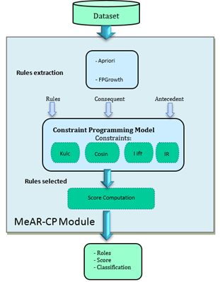
Our MeAR-CP (Evaluation association rules using constraint programming) approach consists of filtering the association rules obtained via the Apriori and FP-Growth algorithms through a constraint programming model, using the chosen null-invariant metrics. Then, we establish a ranking of relevant rules according to a score metrics calculated from Eq. (8) that we propose in this section. The proposed MeAR-CP approach goes through several phases constituting our framework, shown in Figure 1:
Figure 1. Workflow of MeAR-CP
4.1 Association rule extraction phase
After transforming the datasets into binary tables in the pre-processing phase, the association rules were extracted using the Mlxtend library [37], which is a Python library containing useful tools and functions for data mining tasks.
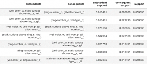
We then used the Apriori and FP-Growth functions of the Mlxtend library in order to find frequent itemsets, and subsequently we used the association rules function to generate the association rules. Figure 2 shows the result of the extraction of rules by the Mlextend library considering a minimum support threshold of 0.5.
Figure 2. Result of rules extraction by Mlextend library
4.2 Constraint programming model
In this step, we consider that for each rule, the corresponding support is already calculated as well as the support of the antecedent and the consequent in the previous step.
To introduce a constraint-programming model, both an objective function and constraints should be mentioned. To achieve this, we introduce three vectors $x, y$ and $z$ of $\mathrm{N}$ size $(\mathrm{N}$ represents the number of rules) in Eq. (7).
- $x=\{x 1, \ldots, x n\}$ will contain the numeric percentage values of the supports of the antecedents of each rule.
- $y=\{y 1, \ldots, y n\}$ will contain the numeric percentages of the supports of the consequences of each rule.
- $z=\{z 1, \ldots, z n\}$ will contain the numeric percentage values of the supports of the entire rule $(x \cup y)$.
Two other variables are also used, the variable $R=\{r 1, \ldots$, $r n\}$, represent the rules and $s$ represent the minimum threshold used in constraints.
The constraint programming model utilized an objective statement, as shown in Eq. (7), aiming to discover a set of rules R that adhere to all predetermined constraints. This model can be expressed as follows:
Objective: Identify a set of rules R that satisfies all constrains. For each rule $\boldsymbol{r}_i$ in set R, the constraint can be formulated as follows:
$\begin{aligned} &\ \ \ \ Kuls\ \left(r_i\right)=\frac{1}{2}\left[\frac{support(z i)}{support(x i)}+\frac{support(z i)}{support(y i)}\right]>s_{Kuls} \\ &\ \ Cosine\ \left(r_i\right)=\left[\frac{\mid support(z i) \mid}{\sqrt{support(x i) * support(y i)}}\right]>s_{Cosine} \\ &\ \ \ \ \ Lift\ \left(r_i\right)=\left[\frac{support(zi)}{support(x i) * support(y i)}\right]>s_{Lift} \\ & IR\ \left(r_i\right)=\left[\frac{\mid support(x i)\text{_}{support(y i) \mid}}{support(x i)_{+} support(y i)-support(z i)}\right]<s_{I R} \\ & \end{aligned}$ (7)
where, $SMesure$ is the specified thresholds for each measure.
The proposed constraint-programming model is used to ensure the positive correlation of the itemsets constituting the rules (step 1), thus eliminate the rules deemed irrelevant from the start in order to reduce the execution time.
4.3 Score metrics
Knowing that the IR value [30] increases relatively in relation to the imbalance in the frequency of appearance between the antecedent and the consequent of the rule. Substraction of this value allows us to favour balanced itemsets. Indeed, for the threshold values of Kulczynski [38] and Cosine [28], we obtain the best possible rules. While on the IR side we will look for the minimum threshold value in order to obtain the best possible rules (balanced rules).
$Score\ (r)=\frac{Kuls(r)+Cosine(r)}{2}-IR(r)$ (8)
The objective is to maximize the value of the Score, our model will seek to maximize the latter by taking into account the maximum values of Kulczynski and Cosine, and the minimum value of IR. Hence the formula presented in Eq. (8) which allows us to generate high scores when the conditions of maximization of Kulczynski and Cosine, as well as minimization of IR are met.
We implemented an algorithm for each measurement we used (Kulczynski, Imbalance Ratio, Cosine, Lift), these algorithms follow a generic scheme like the algorithm presented in Algorithm 1. This algorithm calculates the value of each metric according to its mathematical formula and then compare them to a predefined threshold. If the values are lower (or higher for IR) than the fixed threshold, they will not be taken into account.
|
Algorithm 1: Generic algorithm (IR) |
|
1. Input: $r=\{r 1, \ldots, r n\}, x=\{x 1, \ldots, x n\}, y=\{y 1, \ldots, y n\}, z=\{z 1, \ldots,z n\}, s_{I R}$ 2. Output: r 3. Measure = *Mathematical formula of the measure* 4. If Measure < threshold then 5. Measure > threshold in IR case 6. Domain(r).retrieve(r.current value()); 7. Return fault; 8. End 9. Else measure ≥ threshold then 10. Measure ≤ threshold in IR case 11. Return true; 12. End 13. return undefined 14. Domain(r).nextValue() 15. End |
A Score is assigned to each rule retained in order to determine its degree of validity and relevance. The Score is calculated as shown in the Algorithm 2:
|
Algorithm 2: Computing score of the solutions |
|
1. Input: $r=\{r 1, \ldots, r n\}, x=\{x 1, \ldots, x n\}, y=\{y 1, \ldots, y n\}, z=\{z 1, \ldots,z n\}, zn$ 2. Output: r 3. modelCP.addConstraint (Kulc(r, x, y, z, s)) ; 4. modelCP.addConstraint (Cosin(r, x, y, z, s)) ; 5. modelCP.addConstraint (Lift(r, x, y, z, s)) ; 6. modelCP.addConstraint (IR(r, x, y, z, s)) ; 7. while modelCP.findSolution do 8. $Score\ (solution)=\frac{Kuls(solution)+Cosine(solution)}{2}-IR(solution)$ 9. End |
In this section, we introduced the constraint-programming model. This model is executed after extraction of the association rules, it is based on null-invariant metrics and allows us to evaluate the correlation between the itemsets of these rules. Then we proposed a formula allowing us to calculate a score for each rule accepted by the constraint-programming model.
In the following section, we will choose a few datasets of different sizes to perform experiments with our MeAR-CP algorithm in order to measure its effectiveness and observe its execution.
In this section, we present the tests and experiments we performed on some real datasets to evaluate our constraint programming model and the effectiveness of the proposed score formula. We show firstly the characteristics of the datasets used, secondly the development environment and precisely the results of the tests carried out on these datasets.
5.1 Datasets
In order to examine the behavior of our algorithm and make a clear comparison, our experiments were carried out on authentic datasets. The selected datasets are those from UCI Machine Learning Repository and Frequent Itemset Mining Dataset Repository [39]. Table 6 illustrates the different information of each dataset, including the total number of transactions, the total number of attributes, classes, Items nature, Domain and the dataset's density, which is calculated as the average number of items per transaction divided by the number of items.
Table 6. Dataset characteristics
|
Data set |
Mushrooms |
Chess |
BMS WebView 1 |
Connect |
Accidents |
|
Transactions number (T) |
8124 |
3196 |
59602 |
67557 |
340183 |
|
Classes |
2 |
3 |
/ |
2 |
2 |
|
Items number (I) |
22 |
75 |
497 |
129 |
468 |
|
Items nature |
categorical |
categorical |
categorical |
categorical |
categorical |
|
Density |
19.33% |
49.33% |
0.51% |
33.33% |
7.22% |
|
Domain |
Classification |
datamining |
datamining |
datamining |
datamining |
5.2 Dense database
The number of items is small compared to the number of transactions, the random distribution of items on transactions gives us records that “look similar”. This means that the number of itemsets will be relatively small.
5.3 Sparse database
Transactions are more diverse, with a greater variety of items, and would result in a higher number of itemsets. The more the number of items increases in a database (for the same number of transactions), the less dense it is, and the sparser it is.
5.4 Development environment
To solve our constraints, we used Choco-solver, which is Java library for constraint programming [6, 40].
The Choco library contains several predefined constraints, it is also possible to create your own constraints. Users can describe problems in a declarative way (objective statement), listing constraints that should be satisfied in each solution. The problem is then solved automatically by combining filter algorithms with a search space exploration mechanism.
The solver has the ability to identify the solution(s) if they are present. In the case the problem does not allow any solution, the solver will ascertain that the equation is incapable of being solved.
5.5 Results
To evaluate the performance of our technique, we tested our algorithms considering execution time and the number of relevant rules extracted. In our experiments, the data sets used are from UCI. Initially, we experimented with five data sets to assess time execution and memory consumption, evaluating the impact when introducing our method within the extraction algorithm. Subsequently, we evaluated both execution time and the rules extracted while varying the threshold of all metrics. Finally, we compute the average Score for all data sets. In the remainder of this section, we present these scenarios.
First scenario
One of the fundamental characteristics of any data-mining algorithm is its ability to demonstrate efficiency and minimize memory usage. Considering those factors, we measured execution time and memory usage during our experiments. Table 7 presents a comparison of the execution time, measured in seconds, of the Apriori and FP-Growth algorithms, as well as our MeAR-CP evaluation method for different datasets.
Table 7. Runtime (in sec)
|
Dataset |
Apriori |
FP-Growth |
MeAR-CP |
MeAR-CP + Apriori |
MeAR-CP + FP-Growth |
|
Mushrooms |
0.0469 |
0.0399 |
1.062 |
1.108 |
1.101 |
|
BMSWebView 1 |
6.166 |
1.700 |
0.037 |
6.173 |
1.737 |
|
Connect |
7.908 |
7.723 |
0.337 |
8.245 |
8.060 |
|
Chess |
3.501 |
0.465 |
2.669 |
6.170 |
3.134 |
|
Accidents |
30.026 |
24.850 |
2.366 |
32.569 |
27.216 |
According to the results of this Table 7, we observe that our MeAR-CP method demonstrates superior speed when compared to the Apriori and FP-Growth algorithms (with the exception of the Mushrooms dataset). Furthermore, in all scenarios, FP-Growth shows higher efficiency than the Apriori algorithm.
Table 8 presents memory consumption RAM (MB) for our MeAR-CP method across different datasets.
Table 8. Memory consumption (MB)
|
Dataset |
Apriori |
|
Mushrooms |
190 |
|
BMSWebView 1 |
14 |
|
Connect4 |
185 |
|
Chess |
268 |
|
Accidents |
163 |
When examining RAM usage, it becomes evident that there is a rather conservative consumption of RAM, which remains below the threshold of 300 MB.
After careful examination of the execution duration and memory usage of our MeAR-CP method, it becomes clear that we can integrate them seamlessly after implementing the Apriori and FP-Growth algorithms, without significantly affecting the Runtime and RAM consumption.
Second scenario
In this experiment, we will vary the threshold of each metric for every dataset while quantifying the execution time and the number of rules identified.
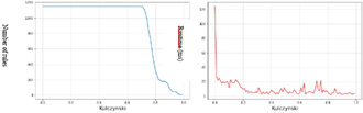
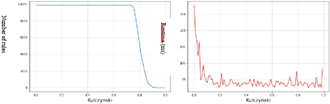
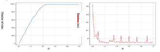
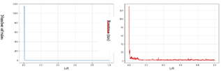
Figure 3. Result of the dataset mushrooms (Kulczynski)
The graphs in Figure 3 show the progression of rules number per Kulczynski threshold variation, as well as the execution time, measured in milliseconds (ms), for the Mushrooms dataset.
In the beginning, the rules number greater than 1100, and then we observe a decrease from the Kulczynski threshold of 0.71. This decrease continues, depending on the Kulczynski threshold value, until reaching 8 rules for the Kulczynski threshold value of 0.99.
As for the execution time, it starts at 124 ms and then gradually decreases until it initially reaching a value of approximately 20 ms, before stabilizing towards a value of 10 ms.
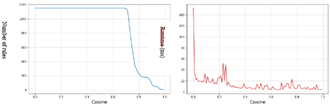
Figure 4. Result of mushrooms dataset (Cosine)
The plots in Figure 4 illustrate the evolution of the number of rules per variation of the Cosine threshold, as well as the time execution, measured in milliseconds (ms), for the Mushrooms dataset.
Initially the number of rules is greater than 1100, then we observe a drop from the Cosine threshold 0.71, and a continuation of this drop depending on the value of the Cosine threshold until reaching 6 rules for a threshold value of Cosine by 0.99.
For the execution time, which starts at 152 ms and subsequently it gradually, decreases until initially reaching a value of approximately 25 ms, before stabilizing towards a value of 8ms.
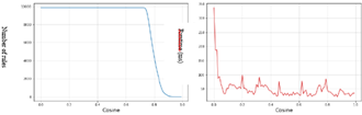
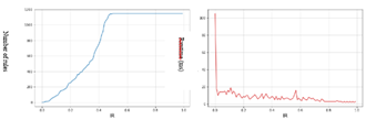
Figure 5. Connect4 dataset result (Kulczynski)
From Figure 5, it is observed that the rules number in the Connect4 dataset, initially greater than 10,000, drops below the Kulczynski threshold of 0.74. This decline persists based on the Kulczynski threshold value until it reaches 0 rules, with a threshold value of Kulczynski set at 0.97. For the execution time, which starts at 277 ms and subsequently it gradually, decreases until initially reaching a value of approximately 30 ms, before stabilizing towards a value of 30 ms.
Figure 6. Result of Connect4 dataset (Cosine)
The progression of the rules number per variation of the Cosine threshold, as well as the time execution, measured in milliseconds (ms), for the Connect4 dataset is shown in Figure 6.
According to this figure, the number of rules at the beginning is close to 10,000 and it remains stable up to a Cosine value of 0.73 where we see a drop, which persists with the evolution of the Cosine value until reaching 0 rules from a value of Cosine of 0.97. On the other hand, the execution time is above 340 ms and thereafter it gradually decreases until it stabilizes around a value of 35 ms.
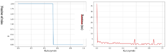
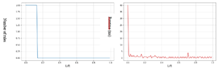
Figure 7. Result of BMS1 dataset (Kulczynski)
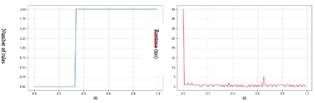
Figure 7 represents the evolution of rules number per variation of the Kulczynski threshold, as well as the time execution, measured in milliseconds (ms), for the BMS1 dataset.
At the beginning the number of rules is equal to 2 and it remains stable up to a Kulczynski threshold of 0.54 where it drops directly to 0 rules and it remains at this value for the rest of the Kulzcynski threshold.
The initial execution time is 37 ms and we immediately notice a drop towards a value of 1ms, where it remains stable until the end of the program.
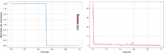
Figure 8. Result of BMS1 dataset (Cosine)
Figure 8 illustrates the progression of the rules number variation of the Cosine threshold, and the time execution, measured in milliseconds (ms), for the BMS1 dataset.
The number of rules start at 2 rules and it remains stable up to a Cosine threshold of 0.51 where it immediately drops to 0 rules and it remains inert for the rest of the Cosine threshold values. As for the execution time, it is initially close to a value of 45 ms then instantly drops to a value of 1ms, where it remains stable until the end of the program.
Figure 9. Result of the Connect4 dataset (IR)
Figure 9 represents the evolution of the rules number per variation of the IR threshold, as well as the time execution, measured in milliseconds (ms), for the Connect4 dataset.
It represents the evolution of the number of rules by variation of the IR threshold, as well as the execution time of our method MeAR-CP in ms for the Connect4 dataset.
Initially, the number of rules is 112 rules then, we observe a progressive increase from the value of the threshold 0.03 of IR, and a continuation of this increase according to the value of the threshold of IR, until reaching a number of solutions close to 10,000 rules from an IR value of 0.45. While the execution time starts at 260 ms and then gradually decreases until it stabilizes around a value of 25 ms.
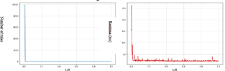
Figure 10. Result the dataset Mushrooms (IR)
Figure 10 shows the progression of the rules number per variation of the IR threshold and the time execution, measured in milliseconds (ms), for the Mushrooms dataset.
In the beginning, the number of rules is 0, then we notice a progressive rise from the IR threshold value of 0.02, and a continuation of this rise depending on the IR threshold value until reaching a number of rules close to 1200 rules from an IR value of 0.50. On the other hand, the execution time starts at 105 ms and immediately drops to stabilize around a value of 5 ms.
Figure 11. Result of BMS1 dataset (IR)
The progression of the rules number per variation of the IR threshold and the time execution (in milliseconds; ms), for the BMS1 dataset are shown in Figure 11. From these results, the number of rules is 0 at the beginning, and continues until the threshold value 0.34 where the number of rules increases to 2, and remains like this despite the evolution of the IR threshold value.
As for the execution time, it is initially 40 ms then it drops to stabilize around 1 ms.
Figure 12. Result of Connect4 dataset (Lift)
The graphs in Figure 12 illustrate the progression of the number of rules per variation of the Lift threshold, as well as the time execution, measured in milliseconds (ms), for the Connect4 dataset. At the beginning, we notice that the number of rules is close to 10000, and then it immediately drops to 0 with the progression of the Lift threshold value. The execution time initially is 260 ms then it drops directly to remain inert around a value of 20 ms.
Figure 13. Résultat du dataset Mushrooms (Lift)
Figure 13 shows the evolution of the rules number and execution time as a function of the Lift threshold for the Mushrooms dataset.
From these figures, we notice initially that the number of rules is above 1100, and then we notice an immediate descent to 0 with the progression of the Lift threshold value. As for the execution time, is initially at 130ms, and then it drops instantly to remain stable around a value of 2ms.
The graphs in Figure 14 illustrate the progression of the rules number and execution time per variation of the Lift threshold for the BMS1 dataset.
Figure 14. Result of BMS1 dataset (Lift)
The number of rules is equal to 2 at the beginning, subsequently we observe a descent to 0 after a Lift value of 0.1. The execution time initially is 40 ms then it drops directly to stabilize around a value of 1ms.
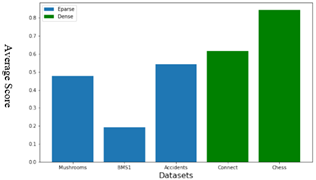
Third scenario
In the last experiment, we varied the Score threshold for the five datasets, and computed the average Score for each dataset. Figure 15 shows the average Score obtained for each dataset.
Figure 15. Average score by dataset
Discussion and Analysis
The reduction in the number of rules is explained by the increase in the threshold of each metric, the higher the threshold value, the more the number of rules will drop significantly (elimination rules irrelevant to the metric) until reaching a minimum for the highest values of the threshold as shown in Figures 3-8.
The reduction in execution time is explained by the fact that initially the program will first initialize the data used (reading the data, creating the programming model by constraints, initializing the solver) which explains the significant time at start of execution. This time will go down once these execution steps are completed.
According to the different results obtained, we deduce that the Cosine measure is stricter than the Kulczynski measure because it eliminates more rules despite an equivalent threshold.
The rules number initially is very low as shown in Figures 9-11. This is explained by the small value of IR, so the algorithm only takes into account very balanced rules.
That is, the higher the IR threshold value, the more the algorithm will retain less balanced rules and therefore the number of solutions will increase.
The number of rules drop immediately, despite the very low Lift threshold as shown in Figures 12-14. This is explained by the very strong sensitivity of Lift towards the number of nul transactions (do not contain the itemset) in the datasets used. This sensitivity causes a distortion in the Lift calculation, making it insufficient to evaluate the relevance of the association rules.
The outcomes obtained in Figure 15 allow us to have an overall idea of association rules relevancy:
For the BMS1 dataset, we observe a particularly low average, so the set of rules retained by the algorithm is considered less relevant. Concerning Chess dataset, the average score is relatively high, indicating the relevance of the entire set of rules. As for the Mushrooms, Accidents and Connect4 datasets, their result is close to average.
Advantages
Since the average of the scores reflects the degree of relevance of the set of rules; in the case of a low average (value less than 0.5), it is possible to improve the scores of each dataset by increasing the value of the threshold at the level of our constraint programming model.
After these experiments, we conclude that Lift metric is insufficient for evaluating the relevance of the association rules
Limitations to be further explored
In the future, we plan to explore additional extraction algorithms to assess these rules using Constraint Programming (PPC). We also intend to assess fuzzy rules by integrating fuzzy extraction algorithms into our method. Consequently, additional metrics will be chosen to address the aspect of fuzzy rules.
The key point of this section is on interpreting and evaluating of our method MeAR-CP. To achieve this, we first provided an explanation of the datasets used in the experiment, and then we also evaluated the method in terms of execution time and RAM usage.
Secondly, we observed the behavior of our method MeAR-CP according to the chosen measurements in terms of number of rules and execution time for different datasets. We also presented a comparative result of the score calculations carried out on each dataset.
In the present study, we tackled the challenge of evaluating the relevance of association rules in an efficient manner. For this purpose, relevant metrics were selected to be utilized in our process. Then, the chosen metrics (Kulczynski, Cosine, IR, Lift) have been modeled as a constraint-programming model using the Choco-solver. New metric called Score was proposed to strengthen our evaluation. The objective being to maximize the value of the Score, our model will seek to maximize the latter by taking into account the maximum values of Kulczynski and Cosine, and the minimum value of IR. In order to have a clear and precise idea of the behavior of our algorithm in relation to different datasets, the results of the experiments were projected in the execution time and the number of rules obtained.
In summary, the BMS1 dataset exhibits a notably low average, suggesting that the set of rules identified by the algorithm may be less relevant. Conversely, for the Chess dataset, the average score is relatively high, indicating the significance of all extracted rules. However, the results for the Mushrooms, Accidents, and Connect4 datasets are in line with the average.
In light of the satisfactory results obtained and the findings of this study, several other metrics could be investigated. Additionally, multiple extraction algorithms could be employed. Furthermore, adapting these metrics to fuzzy datasets using the same methodology.
We thank the Directorate-General for Scientific Research and Technological Development (DGRSDT), for its support of this research work.
[1] Shamie, M.M., Almustafa, M.M. (2021). Improving association rule mining using clustering-based data mining model for traffic accidents. Review of Computer Engineering Studies, 8(3): 65-70. https://doi.org/10.18280/rces.080301
[2] Kamepalli, S., Bandaru, S. (2019). Weighted based frequent and infrequent pattern mining model for real-time E-commerce databases. Advances in Modelling and Analysis B, 62(2-4): 53-60. https://doi.org/10.18280/ama_b.622-404
[3] Pasquier, N. (2000). Extraction de Bases pour les Règles d'Association à partir des Itemsets Fermés Fréquents. In Inforsid'2000 Congress, pp. 56-77. https://hal.archives-ouvertes.fr/hal-00467753.
[4] Gorawski, M., Siedlecki, Z. (2011). Implementation, optimization and performance tests of privacy preserving mechanisms in homogeneous collaborative association rules mining. In On the Move to Meaningful Internet Systems: OTM 2011: Confederated International Conferences: CoopIS, DOA-SVI, and ODBASE 2011, Hersonissos, Crete, Greece, October 17-21, 2011, Proceedings, Part I, pp. 347-366. https://doi.org/10.1007/978-3-642-25109-2_23
[5] Lenca, P., Meyer, P., Picouet, P., Vaillant, B., Lallich, S. (2003). Critères d'évaluation des mesures de qualité des règles d'association. Revue des Nouvelles Technologies de l'Information, 123-134. https://hal.science/hal-00632772/.
[6] Jussien, N., Rochart, G., Lorca, X. (2008). Choco: An open source java constraint programming library. In CPAIOR'08 Workshop on Open-Source Software for Integer and Contraint Programming (OSSICP'08), pp. 1-10. https://hal.science/hal-00483090/
[7] Kim, S., Barsky, M., Han, J. (2011). Efficient mining of top correlated patterns based on null-invariant measures. In Machine Learning and Knowledge Discovery in Databases: European Conference, ECML PKDD 2011, Athens, Greece, September 5-9, 2011, Proceedings, Part II 22, pp. 177-192. https://doi.org/10.1007/978-3-642-23783-6_12
[8] Toivonen, H., Klemettinen, M., Ronkainen, P., Hätönen, K., Mannila, H. (1995). Pruning and grouping of discovered association rules. In ECML Workshop on Statistics, Machine Learning, and Knowledge Discovery in Databases, pp. 47-52.
[9] Tan, P.N., Kumar, V., Srivastava, J. (2004). Selecting the right objective measure for association analysis. Information Systems, 29(4): 293-313. https://doi.org/10.1016/S0306-4379(03)00072-3
[10] Djenouri, Y., Gheraibia, Y., Mehdi, M., Bendjoudi, A., Nouali-Taboudjemat, N. (2014). An efficient measure for evaluating association rules. In 2014 6th International Conference of Soft Computing and Pattern Recognition (SoCPaR), pp. 406-410. https://doi.org/10.1109/SOCPAR.2014.7008041
[11] Dilekh, T., Boulahia, M.A., Benharzallah, S. (2023). Assessing semantic similarity measures and proposing a wup-resnik hybrid metric for enhanced arabic language processing. Revue d'Intelligence Artificielle, 37(5): 1311‑1322. https://doi.org/10.18280/ria.370524
[12] Plasse, M., Keita, N.N., Saporta, G., Leblond, L. (2006). Une comparaison de certains indices de pertinence des règles d'association. In EGC 06 Extraction et Gestion des Connaissances, pp. 561-568. https://hal.science/hal-01125152/.
[13] Dahbi, A., Jabri, S., Balouki, Y., Gadi, T. (2017). A new method to select the interesting association rules with multiple criteria. International Journal of Intelligent Engineering & Systems, 10(5): 191-200. https://doi.org/10.22266/ijies2017.1031.21
[14] Brin, S., Motwani, R., Silverstein, C. (1997). Beyond market baskets: Generalizing association rules to correlations. In Proceedings of the 1997 ACM SIGMOD international conference on Management of data, pp. 265-276. https://doi.org/10.1145/253262.253327
[15] Bayardo Jr, R.J., Agrawal, R. (1999). Mining the most interesting rules. In Proceedings of the fifth ACM SIGKDD international conference on Knowledge discovery and data mining, pp. 145-154. https://doi.org/10.1145/312129.312219
[16] Kemmar, A., Lebbah, Y., Loudni, S., Boizumault, P., Charnois, T. (2016). A global constraint for sequential pattern mining. Revue d'Intelligence Artificielle, 30(6): 675-703. https://doi.org/10.3166/ria.30.675-703
[17] Belaid, M.B., Bessiere, C., Lazaar, N. (2019). Constraint programming for association rules. In Proceedings of the 2019 SIAM International Conference on Data Mining, pp. 127-135. https://doi.org/10.1137/1.9781611975673.15
[18] De Raedt, L., Guns, T., Nijssen, S. (2008). Constraint programming for itemset mining. In Proceedings of the 14th ACM SIGKDD international conference on Knowledge discovery and data mining, pp. 204-212. https://doi.org/10.1145/1401890.1401919
[19] Hien, A., Loudni, S., Aribi, N., Lebbah, Y., Laghzaoui, M.E.A., Ouali, A., Zimmermann, A. (2021). A relaxation-based approach for mining diverse closed patterns. In Machine Learning and Knowledge Discovery in Databases: European Conference, ECML PKDD 2020, Ghent, Belgium, September 14–18, 2020, Proceedings, Part I, pp. 36-54. https://doi.org/10.1007/978-3-030-67658-2_3
[20] Bayardo, R.J., Agrawal, R., Gunopulos, D. (2000). Constraint-based rule mining in large, dense databases. Data Mining and Knowledge Discovery, 4: 217-240. https://doi.org/10.1109/ICDE.1999.754924
[21] Agrawal, R., Srikant, R. (1994). Fast algorithms for mining association rules. In Proc. 20th int. conf. very large data bases, VLDB, pp. 487-499.
[22] Han, J., Pei, J., Yin, Y., Mao, R. (2004). Mining frequent patterns without candidate generation: A frequent-pattern tree approach. Data Mining and Knowledge Discovery, 8: 53-87. https://doi.org/10.1023/B:DAMI.0000005258.31418.83
[23] Jabbour, S., El Mazouri, F.E., Sais, L. (2018). Mining negatives association rules using constraints. Procedia Computer Science, 127: 481-488. https://doi.org/10.1016/j.procs.2018.01.146
[24] Ünvan, Y.A. (2021). Market basket analysis with association rules. Communications in Statistics-Theory and Methods, 50(7): 1615-1628. https://doi.org/10.1080/03610926.2020.1716255
[25] Brin, S., Motwani, R., Ullman, J.D., Tsur, S. (1997). Dynamic itemset counting and implication rules for market basket data. In Proceedings of the 1997 ACM SIGMOD international conference on Management of data, pp. 255-264. https://doi.org/10.1145/253260.253325
[26] Iyigun, C., Moghaddass, R., Oztekin, A. (2016). Grouping association rules using lift. In the 11th INFORMS Workshop on Data Mining and Decision Analytics. https://api.semanticscholar.org/CorpusID:25368371.
[27] Bhattacharyya, A. (1946). On a measure of divergence between two multinomial populations. Sankhyā: The Indian Journal of Statistics, 7(4): 401-406. https://www.jstor.org/stable/25047882.
[28] Ye, J. (2011). Cosine similarity measures for intuitionistic fuzzy sets and their applications. Mathematical and Computer Modelling, 53(1-2): 91-97. https://doi.org/10.1016/j.mcm.2010.07.022
[29] Singhal, A. (2001). Modern information retrieval: A brief overview. IEEE Data Eng. Bull., 24(4): 35-43.
[30] Noorhalim, N., Ali, A., Shamsuddin, S.M. (2019). Handling imbalanced ratio for class imbalance problem using SMOTE. In Proceedings of the Third International Conference on Computing, Mathematics and Statistics (iCMS2017) Transcending Boundaries, Embracing Multidisciplinary Diversities, pp. 19-30. https://doi.org/10.1007/978-981-13-7279-7_3
[31] Wu, T., Chen, Y., Han, J. (2010). Re-examination of interestingness measures in pattern mining: A unified framework. Data Mining and Knowledge Discovery, 21(3): 371-397. https://doi.org/10.1007/s10618-009-0161-2
[32] Ali, A., Shamsuddin, S.M., Ralescu, A.L. (2013). Classification with class imbalance problem: A review. https://www.researchgate.net/profile/Aida-Ali-4/publication/288228469_Classification_with_class_imbalance_problem_A_review/links/57b556d008ae19a365faff16/Classification-with-class-imbalance-problem-A-review.pdf.
[33] Han, J., Kamber, M., Pei, J. (2012). 6-mining frequent patterns, associations, and correlations: Basic concepts and methods. In Data mining, pp. 243-278. https://doi.org/10.1016/B978-0-12-381479-1.00006-X
[34] Singh, S., Yassine, A. (2018). Big data mining of energy time series for behavioral analytics and energy consumption forecasting. Energies, 11(2): 452. https://doi.org/10.3390/en11020452
[35] Rossi, F., Van Beek, P., Walsh, T. (2006). Handbook of constraint programming. Elsevier. https://api.semanticscholar.org/CorpusID:14174798.
[36] Aoga, J. (2019). Global constraints for mining sets and sequences (Doctoral dissertation, UCL-Université Catholique de Louvain). https://dial.uclouvain.be/pr/boreal/object/boreal:218062.
[37] Raschka, S. (2018). MLxtend: Providing machine learning and data science utilities and extensions to Python’s scientific computing stack. Journal of Open Source Software, 3(24): 638. https://doi.org/10.21105/joss.00638
[38] Han, J., Pei, J., Tong, H. (2022). Data mining: Concepts and techniques. Morgan kaufmann. https://api.semanticscholar.org/CorpusID:10539605.
[39] Borgelt, C. (2012). Frequent item set mining. Wiley Interdisciplinary Reviews: Data Mining and Knowledge Discovery, 2(6): 437-456. https://doi.org/10.1002/widm.1074
[40] Prud’homme, C., Fages, J.G. (2022). Choco-solver: A Java library for constraint programming. Journal of Open Source Software, 7(78): 4708. https://doi.org/10.21105/joss.04708