Dhurgham Mohammed Jasim*![]() | Ehab Abdul Razzaq Hussein
| Ehab Abdul Razzaq Hussein![]() | Hilal Al-Libawy
| Hilal Al-Libawy![]()
© 2024 The authors. This article is published by IIETA and is licensed under the CC BY 4.0 license (http://creativecommons.org/licenses/by/4.0/).
OPEN ACCESS
Cathodic protection is a significant approach utilized to avoid the electrochemical corrosion of pipelines. This is accomplished by supplying an electric current to the structure that requires protection, such as a pipeline, from an external source. study aims to enhance the cathodic protection system by minimizing potential fluctuations along the pipeline hence preventing corrosion. It also aims to achieve economic feasibility by decreasing the number of anodes utilized. These objectives were accomplished by employing meta-heuristic optimization techniques. The present study involves formulating a mathematical model for a pipeline that provides fuel to the Al-Hilla 2 power plant in Iraq to assess the effectiveness of cathodic protection. Utilizing numerical simulation techniques, Multiphysics COMSOL, diverse scenarios are examined, resulting in the acquisition of substantial data. Subsequently, a neural network model is constructed using MATLAB. The primary factors influencing the distribution of cathodic protection potential are the numbers and positioning of the anodes and the output current. Subsequently, the optimization objectives involve determining the optimal anode number, position, and output current value by utilizing the Particle swarm organization (PSO) algorithm. The obtained results provide evidence that the proposed method holds a certain level of significance in guiding the design of cathodic protection systems.
cathodic protection, ICCP, pipeline, FEM, metaheuristic algorithm, PSO
The issue of metal corrosion carries significant economic impacts since information shows that industrialized nations allocate roughly 5% of their income towards corrosion prevention, maintenance, and replacement of damaged and polluted products resulting from corrosive reactions.
The corrosion of underground metal pipelines, storage tanks, and different metallic structures is a natural and inherent phenomenon that arises from an electrochemical reaction, wherein a flow of current occurs between anodic regions where corrosion is taking place and cathodic regions where it is not. The cathodic protection system serves to reverse the process, which functions by designating the metallic structure to be protected as the cathode and the sacrificial component as the anode. This arrangement effectively prevents the process of metallic structure corrosion [1]. There are two techniques for cathodic protection: sacrificial anode cathodic protection (SACP) and Impressed Current Cathodic Protection (ICCP). ICCP is the main technique to prevent the corrosion of metallic structures buried in soil. ICCP is a technique employed to mitigate the corrosion of a structure by designating it as the cathode within an electrochemical cell. The technique of corrosion prevention involves the establishment of a connection between the metallic structure that requires protection and a sacrificial metal that is more susceptible to corrosion, serving as the anode. ICCP systems are commonly employed to mitigate corrosion in underground storage tanks and their associated metal pipeline systems [2].
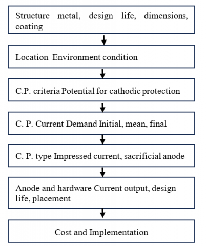
An effectively designed ICCP system as shown in Figure 1 can mitigate these issues, hence ensuring the structural stability of the metallic structures and substantially minimizing maintenance expenses over its operational lifespan. Metallic corrosion refers to an electrochemical process wherein a metal undergoes a chemical reaction with a non-metal, such as oxygen, resulting in the formation of a metal oxide or another compound. The response to the corrosion process is based on the characteristics of the given context. Various metals exhibit varying propensities for corrosion, activity, or potential. The potentials mentioned above can be organized and compiled into a comprehensive electrochemical series [3]. A more practical methodology is to evaluate the ability of specific metals to undergo corrosion in a specific electrolyte, such as soil [4].
The utilization of numerical simulation methods has gained importance as one of the main fields of research due to the rapid advancements in computer technology and electrochemical technology [5, 6]. The utilization of calculating programs or established software can facilitate the simulation of complicated influencing aspects, hence offering a robust safeguard against corrosion.
Numerical approaches, such as the boundary element method (BEM) [7], have gained significant traction among researchers and corrosion engineers for modeling and resolving diverse corrosion issues [8-10]. The mathematical model for the cathodic protection of pipelines utilizing a typical anode arrangement was constructed, incorporating non-uniform current distributions [11]. The authors of reference [12] conducted a study on the various elements that influence interference in cathodic protection. They analyzed these issues using the BEASY program, specifically the Boundary Element Method (BEM). The analysis of the optimal electrode position for the cathodic protection sacrificial anode system in pipelines was conducted by utilizing the Boundary Element Method (BEM) with the aid of MATLAB® software, as described in reference [13].
This study examines the optimal distance between the pipeline and sets of anodes, as well as the impact of varying key parameters on the potential distribution on the pipeline surface that is safeguarded through cathodic protection utilizing mixed metal oxidation (MMO) sacrificial anode. Mixed Metal Oxide (MMO) anodes are effective in various conditions such as soil, freshwater, mud, and marine environments. The anodes' coatings exhibit great chemical stability and remain unaffected by chlorination. Moreover, the anode's small size, measuring approximately one inch in diameter, facilitates the installation procedure as compared to alternative anode varieties. MMO anodes offer a cost-effective solution for any project due to their constantly low resistance, which is attributed to their low consumption rate.
To accomplish this analysis, the utilization of a approach involving the finite element method (FEM) and particle swarm optimization algorithm (PSO) is implemented.
Figure 1. Cathodic protection design
Out of the many computer simulation software options available, COMSOL is widely recognized as the most popular platform. It enables users to model and simulate physical fields using advanced digital techniques. In addition, the COMSOL program encompasses over 30 modules, one of which is the corrosion module. This module enhances the modeling capabilities for a wide range of physical fields.
The modeling program utilized in this work is COMSOL Multiphysics® version 5.6, which employs FEM as the numerical method. The utilization of the FEM in this study was preferred over alternative methods like the Finite Difference Method (FDM) or the Boundary Element Method (BEM) due to the inclusion of spatially variable governing characteristics, such as the number and location of anodes, as well as the injected current. The Finite Difference Method (FDM) exhibits limited resolution capabilities and encounters challenges when dealing with irregular meshes and nonlinear effects. On the other hand, BEM is unable to effectively address the spatially variable properties of the soil medium being represented in this particular context [5]. Finite Element Method (FEM) study considers both the primary current distribution associated with the resistivity of the electrolyte and the secondary current distribution associated with electrode reactions. Protection conditions are met at every location of the pipeline when the cathodic current density matches the protection current density and the potential falls within the appropriate protection range. The correlation between current density and potential at the metal-electrolyte interface is dependent upon electrode reactions and generally exhibits non-linear behavior. The Finite Element Method is a computational approach used to solve boundary value problems. It optimizes a function that measures error, resulting in a stable solution. The software solves elementary equations within limited subdomains, known as finite elements, to provide an approximation of a more complicated equation across a broader domain.
Boundary conditions are determined by taking into account the electrochemical properties of the metal surface and its protection, which can be achieved by employing the Tafel equations. The solution to the electrical field is obtained by analyzing the Laplace equation [14].
The boundary conditions in the cathodic protection system are typically non-linear due to the absence of linear functional relationships between the protection current density and the associated potential, caused by the electrochemical processes. It is necessary to include certain boundary requirements to restrict and reflect the current conditions. There exist three distinct categories of boundary conditions for cathodic protection systems:
The first boundary condition: soil boundary $\Gamma_{\infty}$.
$\left\{\begin{array}{c}\left(\varphi \mid \Gamma_{\infty}=0\right) \\ \left(i \left\lvert\, \Gamma_{\infty}=-\sigma \frac{\partial^2 \varphi}{\partial n}=0\right.\right)\end{array}\right.$ (1)
The second type of boundary condition: ground boundary $\Gamma_g$.
$\left(i \left\lvert\, \Gamma_g=-\sigma \frac{\partial^2 \varphi}{\partial n}=0\right.\right)$ (2)
The third type of boundary conditions: the boundary conditions of the pipeline surface $\Gamma_P$.
$\Gamma_P=f\left(u-u_{e q}\right)$ (3)
Consider the following as the polarization curve for the cathode:
$\begin{aligned} i=\left[10^{\frac{V-\varphi-E_{F e}}{\beta_{F e}}}\right. & -\left(\frac{1}{\left(1-\alpha_{b l k}\right) \cdot i_{\text {lim }, o_2}}\right. \left.\left.-10^{\frac{V-\varphi-E_{O_2}}{o_2}}\right)^{-1}-10^{\frac{-\left(V-\varphi-E_{H_2}\right.}{\beta_{H_2}}}\right]\end{aligned}$ (4)
v represents the potential of the pipeline. Φ represents the potential of the soil close to the pipeline. The symbol $\beta_{F e}$ denotes the Tafel slope, which characterizes the rate of change of the corrosion reaction. On the other hand, $E_{F e}$ represents the equilibrium potential, which indicates the balance point of the corrosion reaction.
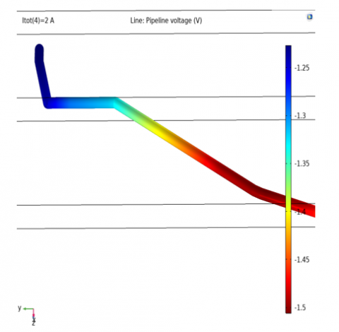
The utilization of Finite Element Method (FEM) enables the accurate representation of complex structural geometries and facilitates the examination of numerous influential factors. The aforementioned tool serves as a valuable asset in the field of CP design, as it enables an evaluation of the effects and consequences of design choices on pre-existing systems and the ability to anticipate various potential outcomes [15]. Figure 2 displays a graphical representation of an underground CP-pipeline system that has been sectioned to show its three-dimensional (3D) structure.
Figure 2. Potential distribution of the dry gas pipeline
The numerical model utilized in this study was derived from the physical model developed within the Multiphysics COMSOL software platform. The Poisson distribution can be used to represent the potential distribution of CP.
$\Delta^2 v=\left(\frac{\partial^2 v}{\partial x^2}+\frac{\partial^2 v}{\partial y^2}+\frac{\partial^2 v}{\partial z^2}\right)=-i / K$ (5)
κ represents the electrolyte conductivity. The model mentioned above can exhibit fluctuations in temperature, which can subsequently impact the conductivity of the electrolyte. In addition, the mathematical expression for the potential field in a uniform electrolyte can be obtained by employing Laplace's equation [16].
$\Delta^2 v=\left(\frac{\partial^2 v}{\partial x^2}+\frac{\partial^2 v}{\partial y^2}+\frac{\partial^2 v}{\partial z^2}\right)=0 \quad((x, y, z) \in \Omega$ (6)
The solution for the distribution of electric potentials can be expressed in the following manner by utilizing Galerkin's weighted residuals approach [17].
$[H]^{F E M} \cdot(\varphi)^{F E M}=(Q)^{F E M}$ (7)
The parameter $[H]^{F E M}$ denotes a two-dimensional matrix consisting of coefficients, with the associated term being specified by:
$\begin{array}{r}h_{i j}^{F E M}=\sum_{e=1}^{n_e} \sigma \int\left(\frac{\partial N_i^e}{\partial x} \frac{\partial N_j^e}{\partial x}+\frac{\partial N_i^e}{\partial y} \frac{\partial N_j^e}{\partial y}\right. \left.+\frac{\partial N_i^e}{\partial z} \frac{\partial N_j^e}{\partial z}\right) d V \\ \left(\left(i=1,2, \ldots, n_f\right)\left(j=1,2, \ldots, n_f\right)\right.\end{array}$ (8)
$(\varphi)^{F E M}$ - The column vector matrix is utilized to denote the unknown potentials present in the nodes of a finite element. The ordinal value of the element is equal to $n_f X 1$.
$(Q)^{F E M}$ - The matrix in column vector form represents the free terms associated with Neumann boundary conditions. The ordinal value of the element is determined by:
$q_i^{F E M}=-\sum_{e=1}^{n_e}\left\lceil\sum_{j=1}^{n_f}\left(\int \sigma N_i^e \cdot N_j^e \cdot \frac{\partial \varphi_j^{F E M}}{\partial n} d s\right)\right]$ (9)
$N_i^e$ - The utilization of shape functions is employed to approximate the unknown potential function in the succeeding way:
$\varphi^{F E M} \sum_{j=1}^{n_f} N_j^e \cdot \varphi_j^e$ (10)
$\frac{\partial \varphi_j^{F E M}}{\partial n}$ - Neumann boundary condition.
A pipeline provides dry gas to Al-Hilla 2 power plant spanning a distance of 26 kilometres was a case study for this research, the location in southern Baghdad, Iraq. The pipeline was installed at a depth of two meters below the surface. The pipeline possesses a diameter measuring 24 inches and a wall thickness measuring 11.13 mm. The material utilized for the pipeline is carbon steel, specifically API 5L Gr.X60. The HDPE material follows a three-layer coating procedure and is then surrounded by a one-meter layer of soil, which produces a resistance of 50Ω•m. Regarding the cathodic protection system, two cathodic protection stations are installed at distances of 6.9 and 13.79 kilometres along the pipeline. Each station has a T/R (transformer/rectifier) with 60 volts and 40 amperes of capacity. T/R provides the pipeline's direct current (DC) voltage. Additionally, there are 20 test points distributed along the pipeline to measure the potential profile for protection. The auxiliary anode is partitioned into two groups, with an output current of 2A. The anodes at each CP station are located at the coordinates (6.9km, 13.79km). Every group comprises 15 anodes composed of Mixed Metal Oxide (MMO).
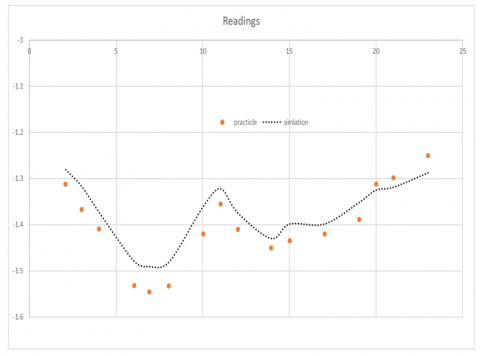
The calculated potential was derived from the mathematical model of the dry gas pipeline using COMSOL computations for, while the actual potential reading of the dry gas pipeline was measured on-site. The current measured reading of the dry gas pipeline was acquired from the test point located directly on the pipeline, as depicted in Figure 3.
Figure 3. Charts of Potential measurement for the dry gas pipeline
The Mean Squared Error (MSE) is considered fairly low and acceptable when the calculated potential responses closely match the actual potential responses.
where, $M S E=\frac{\sum_{i=1}^n\left(y_i-y_i^{\prime}\right)^2}{n}$.
$\text { so } M S E=0.001523 \text {. }$
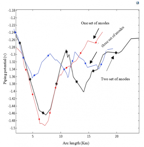
The initial parameters are inputted into the global definition of COMSOL Multiphysics to compute the actual potential of a specific segment of the pipeline. Modifying the quantity, placement, and current output of a sets anodes was made, and an examination of the potential distribution rules was conducted based on the obtained computational outcomes. Figure 4 illustrates the distribution curve of potential with a constant output current, showing different sets of auxiliary anodes. When the number of auxiliary anodes is increased, there is a pattern for the protective potential to be evenly distributed. However, this leads to greater expenses.
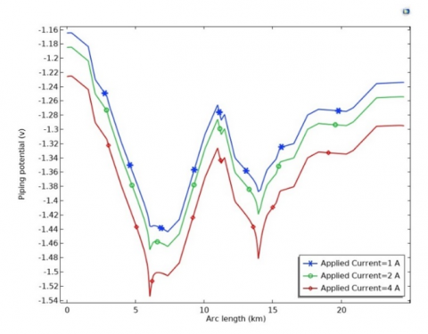
Figure 5 illustrates the potential distribution of a specific group of auxiliary anodes at different levels of electrical currents. When the quantity and placement of auxiliary anodes remain consistent, it is discovered that a relatively uniform potential distribution occurs at a current of 1 A. Nevertheless, it is important to acknowledge that the effectiveness of the protective measures is considerably reduced. When an electrical current of 2A is supplied, the potential distribution demonstrates a level of uniformity that is commonly referred to as "second." However, the observed protective effect has been considered to be superior. The potential distribution demonstrates its most adverse conclusion at an applied current of 4A, which has the potential to result in a hydrogen evolution incident.
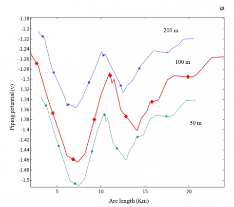
Figure 6 illustrates the distribution of protection potential that arises from adjusting the horizontal distance between the auxiliary anode and the pipeline while keeping all other variables constant. The level of equal distribution in the potential profile reaches a good shape when the auxiliary anode is situated at a distance of 200 meters from the pipeline. The uniformity of the system is modest when the auxiliary anode is positioned at a distance of 100 meters from the pipeline. Nevertheless, the potential profile demonstrates the least amount of consistency when the auxiliary anode is positioned at a distance of 50 meters from the pipeline. The largest magnitude of the cathodic protection effect is observed at a distance of 100 meters from the pipeline. Following this, it can be noted that the influence of cathodic protection is marginally reduced at a distance of 200 meters. It is worth mentioning that a considerable segment of the pipeline, when anodes situated at a distance of 50 meters from the pipeline itself, is presently experiencing elevated levels of cathodic.
Figure 4. CPS potential distribution under different sets of anodes
Figure 5. CPS under different anodes’ current
A set of COMSOL outputs was used to train the neural network. These outputs represent variables that affect the potential distribution along the pipeline and the improvement of cathodic protection. These variables (number of anodes, anode current, and anode position) have a direct and significant impact on the potential distribution, as demonstrated in Figures 4, 5, and 6. The neural network model closely approximated the COMSOL model, with an MSE of 0.0039. The neural network is a straightforward network containing one hidden layer of 60 neurons. The network receives the number of anodes, anode current, and anodes' position as inputs and generates potential distributions as its output as shown in Figure 7.
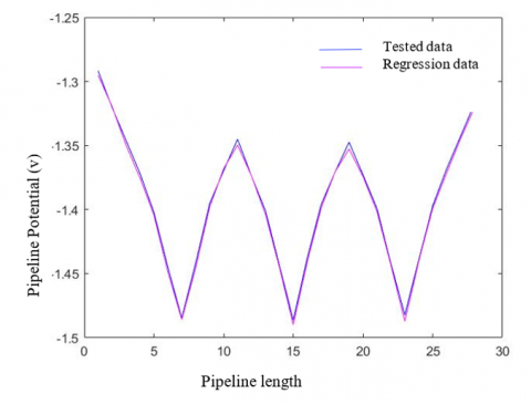
The neural network underwent training using various instances of the outputs generated by the COMSOL program as regression. Subsequently, more cases were employed to examine these outputs. This can be observed in Figure 8, which illustrates the utilization of three sets of anodes.
Figure 6. CPS under different anode positions related to pipeline
Figure 7. Structures of neural network
Figure 8. Predicts and actual data to check the neural network
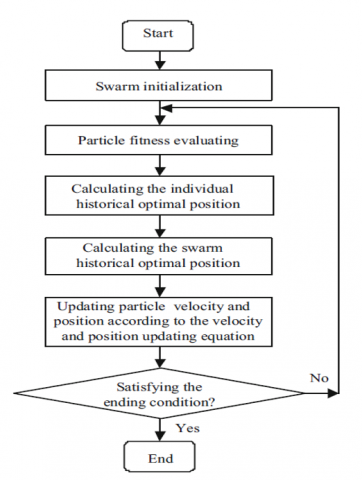
The initial step of the PSO algorithm includes the initialization of the swarm and its associated control settings. In the context of the fundamental PSO algorithm, it is essential to define the acceleration constants, denoted as C1 and C2, as well as the initial velocities, particle positions, and individual best positions. Furthermore, it is necessary to specify the size of neighborhoods in the local best PSO algorithm [18].
Typically, the beginning placements of particles are equally distributed across the search space. It is essential to acknowledge that the efficiency of the PSO algorithm is variable on the initial variety exhibited by the swarm. This refers to the extent to which the search space is encompassed and the degree to which particles are evenly dispersed throughout the search area. The PSO algorithm may address issues with finding the optimal solution if some areas of the search space are not adequately explored by the first swarm. The PSO algorithm will successfully identify an optimal solution if the momentum of a particle leads it to explore unexplored regions, given that the particle reaches a new personal best or a position that becomes the new global best. The velocities are initialized randomly, but they mustn't be too large. If the initial velocities are large, they will result in a high initial momentum and consequently, large updates in position. These large position updates may cause the particles to go beyond the boundaries of the search space and may require more iterations for the swarm to converge on a single solution [19].
By utilizing the particle swarm optimization algorithm, the previously mentioned optimization model may be effectively solved, resulting in the determination of the current value, set of anodes, and the position of the auxiliary anode. This solution ensures the achievement of an evenly distributed protective potential. The optimization processes for the auxiliary anode parameter in the particle swarm organization algorithm are outlined below [20].
The fundamental PSO algorithm is affected by various control parameters, including the problem's dimension, the number of particles, the acceleration coefficients, the inertia weight, the neighborhood size, and the number of iterations. The initial diversity of the swarm has a greater impact on the algorithm's performance, assuming that a reliable and uniform initialization scheme is employed to initialize the particles. A substantial aggregation enables more extensive coverage of the search space throughout each iteration. However, an increase in the number of particles leads to a higher computational complexity every repetition. To fully utilize the benefits of both small and big neighborhood sizes, it is recommended to initiate the search process with small neighborhoods and gradually raise the neighborhood size in accordance to the number of iterations. The number of iterations required to achieve an optimal solution is contingent upon the specific situation at hand. An inadequate number of iterations may result in an early end of the search.
The constants c1 and c2 are trust parameters, with c1 representing the self-confidence of a particle and c2 representing confidence in its neighbors. When c1 = c2 = 0, particles continue moving at their current velocity until they reach the edge of the search space. However, in most applications, c1 = c2 is commonly used.
In this studying the following part provides a comprehensive description of the PSO algorithm. Composing the PSO mathematically within the continuous space coordinate system is the following.
Consider the swarm size to be N = 50 (number of bird), bird steps =50 (Maximum number of birds steps), the acceleration coefficients $\left(c_1=1.2\right.$ and $\left.c_2=1.2\right)$ and w = 0.5 (PSO momentum).
The notation $X_i(t)$ is used to represent the position of particle within the search space at a given time step, denoted as t. It is important to remember that unless explicitly specified, t refers to discrete time increments. The displacement of the particle is altered by introducing a velocity, $V_i(t)$, to the present position.
Particle fitness = absolute value (mean (model function) +1.35) + absolute value (max (model function) - min (model function)). Updating the position and velocity of particle as below:
$X_i(t+1)=X_i(t)+V_i(t)$ (7)
$\begin{gathered}V_i(t+1)=w * V_i(t)+c_1 * \text { rand }\left[\text { gbest }-X_i(t)\right] +c_2 * \text { rand }\left[\text { Lbest }-X_i(t)\right]\end{gathered}$ (8)
The program's flow chart is depicted in Figure 9.
Figure 9. Particle swarm organization algorithm
The efficacy of the optimization method is demonstrated through utilizing of the particle swarm optimization (PSO) algorithm on a dry gas pipeline that supplies the AL Hilla 2 power station. When comparing optimized cathodic protection design with the conventional approach in determining the number and placement of anodes, as depicted in Figure 3, the utilization of the optimization algorithm demonstrates evident superiority in minimizing fluctuations. Consequently, it effectively ensures that the pipeline potential remains within the protected range, thereby mitigating the risks of both over and under-protection.
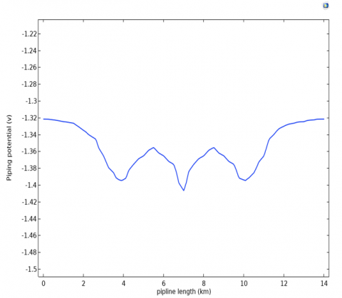
The ultimate outcome of the optimization process shows that the anode output current amounts to 1.91A. Additionally, the anodes are three groups positioned at coordinates (3.91km, 7km, 10.09km) for 14 km pipeline length, each group consist of 5 anodes, with a horizontal distance of 196.6 m. The figure presented in Figure 10 illustrates the optimum potential distribution. The fluctuation of distribution of protection potentials for all pipelines within the protection range is reduced, with a majority of these potentials being.
Figure 10. Protection potential after optimization
This study presents the development of a computational model for calculating the potential of pipeline protection. The model utilizes the Multiphysics COMSOL software to determine the protection potential based on various anode parameters. Based on the computed outcomes, the variables influencing the protection potential distribution of pipeline encompass the quantity of anodes, the positioning of the anodes during installation, and the electrical current of sets of anodes. The objective function is formulated based on the placement of the auxiliary anode and the corresponding output current value. The particle swarm optimization technique is then employed to achieve the optimal solution. The case study provides verification that the utilization of the PSO technique for optimizing anode parameters can enhance the protection potential distribution and the resulting protection effect. PSO utilized the variables that affect the distribution of protection potential along the pipeline's length to determine the optimal variables values for minimizing fluctuation and reducing the number of anodes. This methodology involves using fewer anodes placed at different locations.
Optimization algorithms have a beneficial impact on enhancing the design of cathodic protection systems. These algorithms are capable of identifying the optimal values for the variables that influence the system, resulting in a more precise determination and estimation of the system's operational behavior. Consequently, corrosion can be predicted with greater accuracy in future scenarios.
The utilization of this technology yields economic advantages by maintaining a consistent distribution of potential along the whole length of the pipeline, hence minimizing fluctuations. This results in an extended lifespan of the cathodic protection system, leading to reduced anode replacement intervals, maintenance periods, and excessive current consumption. Furthermore, by an assessment of the anode distribution, it is possible to reduce the number of anodes required, which also proves to be economically viable.
This work is supported by Iraqi Oil Pipelines Company (OPC) / Cathodic Protection Systems Department, State Company for Oil Projects (SCOP) / Engineering Designs Department, and university of Babylon.
|
i |
current density |
|
k |
electrolyte conductivity |
|
API5LGr.X60 |
represent API 5L requirements for high-quality pipe material for the transfer of oil and gas |
|
HDPE |
high density polyethylene |
|
c1 and c2 |
the acceleration coefficients for PSO |
|
N |
number of birds |
|
Xi (t) and Vi (t) |
position and velocity of particle |
|
gbest and lbest |
best global position and best local position |
|
w |
inertia weight used to balance the global exploration and local exploitation |
[1] Guyer, J.P. (2017). An introduction to cathodic protection. The Unified Facilities Criteria of the United States Government, no. 877.
[2] Szabó, S., Bakos, I. (2006). Impressed current cathodic protection. Cathodic Protection, 24(1-2): 39-62. https://doi.org/10.1515/CORRREV.2006.24.1-2.39
[3] Liu, M. (2023). Corrosion and mechanical behavior of metal materials. Corrosion and Mechanical Behavior of Metal Materials, 16(3). https://doi.org/10.3390/ma16030973.
[4] Vasilescu, S.M., Eng, P., Panaitescu, M. (2019). Marine impressed current cathodic protection system. Installation & Instruction Manual C-Shield Marine Impressed Current, 4: 45-62.
[5] Gadala, I.M., Abdel Wahab, M., Alfantazi, A. (2016). Numerical simulations of soil physicochemistry and aeration influences on the external corrosion and cathodic protection design of buried pipeline steels. Materials & Design, 97: 287-299. https://doi.org/10.1016/j.matdes.2016.02.089
[6] Wantuch, A. (2018). Numerical analysis of cathodic protection for traction poles. In 2018 Applications of Electromagnetics in Modern Techniques and Medicine (PTZE), Awice, Poland, pp. 272-275. https://doi.org/10.1109/PTZE.2018.8503251
[7] Del Moral, P. (2020). Theory and applications. Chapman and Hall/CRC. https://doi.org/10.1201/b14924-7
[8] Ridha, M., Safuadi, M., Huzni, S., Israr, I., Ariffin, A.K., Daud, A.R. (2011). The evaluation of cathodic protection system design by using the boundary element method. Advanced Materials Research, 339(1): 642-647. https://doi.org/10.4028/www.scientific.net/AMR.339.642
[9] Izumi, M., Sonohara, M. (2008). Introduction to the feature. Igaku Toshokan, 55(3): 211-211. https://doi.org/10.7142/igakutoshokan.55.211
[10] Fonna, S., Ridha, M., Huzni, S., Ariffin, A.K., Israr, I. (2011). Pre and post processing for Boundary Element Method (BEM) 3D reinforced concrete corrosion simulation. Key Engineering Materials, 462-463: 230-235. https://doi.org/10.4028/www.scientific.net/KEM.462-463.230
[11] Hameed, K.W., Yaro, A.S., Khadom, A.A. (2016). Mathematical model for cathodic protection in a steel-saline water system. Journal of Taibah University for Science, 10(1): 64-69. https://doi.org/10.1016/j.jtusci.2015.04.002
[12] Metwally, I.A., Al-Mandhari, H.M., Gastli, A., Nadir, Z. (2007). Factors affecting cathodic-protection interference. Engineering Analysis with Boundary Elements, 31(6): 485-493. https://doi.org/10.1016/j.enganabound.2006.11.003
[13] Abootalebi, O., Kermanpur, A., Shishesaz, M.R., Golozar, M.A. (2010). Optimizing the electrode position in sacrificial anode cathodic protection systems using boundary element method. Corrosion Science, 52(3): 678-687. https://doi.org/10.1016/j.corsci.2009.10.025
[14] Rodopoulos, D.C., Gortsas, T.V., Tsinopoulos, S.V., Polyzos, D. (017). Boundary element method solution for large scale cathodic protection problems. IOP Conference Series: Materials Science and Engineering, 276(1): 012021. https://doi.org/10.1088/1757-899X/276/1/012021
[15] Protection, C. (2019). Advanced Cathodic Protection Design. https://www.cescor.co.uk/images/Flyers/Advanced_CP_Design_FEM_March_2019.pdf.
[16] Li, C., Du, M., Sun, J., Li, Y., Liu, F. (2013). Finite element modeling for cathodic protection of pipelines under simulating thermocline environment in deep water using a dynamic boundary condition. Journal of The Electrochemical Society, 160(9): E99-E105. https://doi.org/10.1149/2.092309jes
[17] Muharemović, A., Zildžo, H., Letić, E. (2008). Modeling of protective potential distribution in a cathodic protection system using a coupled BEM/FEM method. WIT Transactions on Modelling and Simulation, 47: 105-113. https://doi.org/10.2495/BE080111
[18] Wang, D., Tan, D., Liu, L. (2018). Particle swarm optimization algorithm: An overview. Soft Computing, 22(2): 387-408. https://doi.org/10.1007/s00500-016-2474-6
[19] 16.4 Basic PSO Parameters. https://web2.qatar.cmu.edu/~gdicaro/15382-Spring18/hw/hw3-files/pso-book-extract.pdf.
[20] Slowik, A. (2011). Particle swarm optimization. In Advances in Metaheuristic Algorithms for Optimal Design of Structures, Springer, Cham, pp. 11-43. https://doi.org/10.1007/978-3-319-46173-1_2