Bingyan Wei![]()
© 2024 The author. This article is published by IIETA and is licensed under the CC BY 4.0 license (http://creativecommons.org/licenses/by/4.0/).
OPEN ACCESS
The precise segmentation of different types of brain tumor regions constitutes a critical task in medical image segmentation. Clinically, brain MRI contains abundant information, which can significantly assist doctors in the examination and diagnosis of brain tumor patients. With the advancement of artificial intelligence (AI) and computer technology, some foundational models have increasingly played a pivotal role in the field of computer vision. The Segment Anything Model (SAM) is a fundamental model in the realm of image segmentation, renowned for its exceptional zero-shot segmentation performance and transfer ability, achieving commendable results in natural image processing. To explore the efficacy of SAM in segmenting brain tumor MRI and address the issue of low segmentation accuracy due to uneven image grayscale, a method based on SAM feature fusion is proposed. Features fused from the Transformer and Convolutional Neural Network (CNN) are input into a mask decoder, leveraging the attention mechanism of the Transformer to more effectively capture the global relationships within images, thereby enhancing the precision of the output. Experiments have demonstrated that the method proposed in this study surpasses the segmentation performance of SAM alone, achieving precise segmentation of brain tumor MRI.
brain tumor, image segmentation, segment anything model, feature fusion
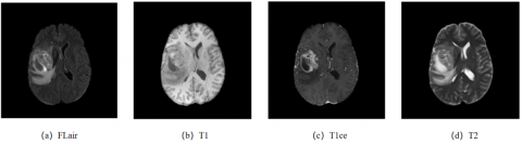
Brain tumors are identified as one of the tumors with exceedingly high incidence and mortality rates, constituting over 85% of all primary central nervous system tumors globally and accounting for approximately 2% to 3% of cancer-related deaths. Such tumors pose a significant threat to human health [1]. Consequently, the early diagnosis and treatment of brain tumors are deemed crucial. In clinical practice, brain MRI is commonly employed for the examination and diagnosis of patients [2]. MRI, a non-invasive imaging technology, is capable of clearly depicting soft tissue lesions and is extensively used in the diagnosis and treatment of brain tumor diseases. To obtain accurate and comprehensive segmentation information, brain tumor segmentation typically requires the utilization of multimodal MRI scan datasets with varying imaging parameters, as illustrated in Figure 1, which presents images of brain tumors in different modalities. These images in varying modalities capture distinct pathological information and can effectively complement each other.
The segmentation of brain tumors in MRI scans is a critical task in medical image segmentation [3]. The objective of brain tumor segmentation is to precisely locate different types of tumor regions within medical images, as demonstrated in Figure 2. The segmented areas include the necrotic tumor core (NCR), the peritumoral edema (ED), and the enhancing tumor (ET). These distinct regions provide vital references for clinical practice. Brain tumors are highly heterogeneous, exhibiting variability in grayscale values and irregularity in shapes within MRI. Therefore, the exploration of precise and reliable methods for brain tumor MRI segmentation represents a challenging endeavor.
Figure 1. Brain tumor images in different modalities
In recent years, with the advancement of AI technology and computational power, foundational models have increasingly played a significant role in the field of natural language processing (NLP), such as Chat-Generative Pre-trained Transformer (GPT) and GPT-4.0 [4]. These large language models have gradually impacted the field of computer vision.
Figure 2. Brain tumor MRI segmentation tasks
Recently, Kirillov et al. [5] introduced the SAM, a foundational model for image segmentation, achieving groundbreaking advancements in the field of computer vision. SAM is celebrated for its exceptional zero-shot transfer capabilities, enabling segmentation of any object within any image without the necessity for any annotations. It has demonstrated commendable results in natural images.
Several researchers have embarked on investigations into the capabilities of SAM in downstream image segmentation tasks. Ding et al. [6] applied SAM to the segmentation of very high resolution (VHR) remote sensing images, proposing the SAM-CD model for change detection (CD) in remote sensing image segmentation and achieving accuracy surpassing that of state-of-the-art (SOTA) methods. Ahmadi et al. [7] utilized SAM for the assessment of civil infrastructure, employing SAM to detect cracks in concrete structures. By integrating SAM with the U-net model, more accurate and comprehensive crack detection results were obtained. These studies indicate that fine-tuning and improvements to SAM can enhance its segmentation performance in downstream tasks. However, due to the complexity and specificity of medical image segmentation tasks, the suitability of SAM for medical image segmentation requires further exploration.
Therefore, this study investigates the segmentation performance of SAM in brain tumor MRI, examining the effectiveness of SAM in the brain tumor MRI segmentation. To enhance the precision of brain tumor MRI segmentation and augment the generalizability of medical image segmentation, a method based on SAM is proposed. After outputting features from the image encoder, Transformer features are reshaped through feature mapping. Then, CNN features are obtained through three layers of 3*3 convolution operations. To better fuse local and global features, a Feature Fusion Block (FFB) is employed between CNN and Transformer features for feature fusion and correction, resulting in fused features with superior representational capability. Experimental results demonstrate that the method proposed herein achieves better segmentation accuracy compared to the SAM alone.
2.1 Foundation model theory
In recent years, AI large models have seen rapid development in the field of NLP. AI large models are short for "AI pre-training large models," and they encompass "pre-training" and "large models," combining to introduce a new paradigm in AI. Specifically, models undergo pre-training on large-scale datasets, enabling them to support various applications directly without the need for fine-tuning or with minimal data adjustment. In 2021, Bommasani et al. [8] proposed the concept of foundation models. Models based on self-supervised learning showcase diverse capabilities throughout the learning process. These capabilities provide both momentum and theoretical underpinnings for downstream applications, leading to the designation of these large models as foundation models.
The advent of foundation models has significantly enhanced the generalization capabilities of models, allowing them to process target tasks from different sources. Numerous milestone models have been introduced to date. In the NLP domain, the most renowned foundation models are the GPT series developed by OpenAI [9]. Adopting a pre-training plus fine-tuning approach, models trained on extensive corpora have demonstrated outstanding performance across a variety of NLP tasks, including text classification, machine translation, and summary generation. With the rapid development of NLP and multimodal fields, several emerging foundation models have been proposed in the field of computer vision.
2.2 SAM
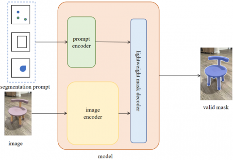
In April 2023, Kirillov et al. [5] introduced the SAM, a foundational model for image segmentation. Designed and trained to be promptable, SAM has been demonstrated to facilitate zero-shot transfer to new image distributions and tasks, achieving instance segmentation without the need for any annotations, and has produced commendable results in natural images [10]. The framework of the SAM is depicted in Figure 3.
SAM transforms segmentation into three main issues: task, model, and data, intertwining these components. Initially, SAM defines a segmentation task that is sufficiently universal to provide a robust pre-training objective. It includes a prompt encoder and combines these two sources of information within a lightweight mask decoder for predicting segmentation masks. Subsequently, the model is trained using a diversified, large-scale dataset.
Following the introduction of SAM, numerous researchers have explored its segmentation capabilities. For instance, to enhance SAM's interactivity, Dai et al. [11] proposed SAMAug, which generates additional point prompts without requiring further manual intervention on SAM. To reduce SAM's inference time, Zhang et al. [12] introduced the EfficientViT-SAM, replacing SAM's image encoder with EfficientViT and thoroughly evaluating it across a series of zero-shot benchmarks. EfficientViT-SAM offers significant improvements in performance and efficiency over all previous SAMs. Song et al. [13] proposed the scalable bias attention mask for SAM (BA-SAM) to enhance SAM's adaptability across different image resolutions without the need for structural modifications. Through several rounds of fine-tuning on downstream tasks, BA-SAM achieves state-of-the-art accuracy across all datasets. Rajič et al. [14] effectively extended SAM's capabilities to the video domain, introducing the SAM-Point Tracking (PT) model for object tracking and segmentation in dynamic videos. SAM-PT utilizes sparse point selection and point propagation techniques to generate masks, leveraging local structural information unrelated to object semantics. Experimental results demonstrate that SAM-PT can produce robust zero-shot performance on popular video object segmentation benchmarks, including DAVIS, YouTube-VOS, and MOSE.
Figure 3. Framework of the SAM
2.3 Application of SAM in medical image segmentation
The advantages of the SAM in the field of natural image segmentation are evident. The transferability and zero-shot segmentation capabilities of SAM are of significant importance for medical imaging, suggesting that SAM's application in medical image segmentation could effectively assist physicians in automated disease diagnosis and screening. Several researchers have explored the role of SAM in medical image segmentation, applying it to downstream segmentation tasks.
Zhang and Wang [15] evaluated the performance of SAM in BraTS2019 dataset. It was found that there is still a gap between SAM and the SOTA models without any model fine-tuning. Zhang and Jiao [16] discussed the potential for SAM in future medical imaging, indicating that SAM does not yield satisfactory segmentation results in many publicly available medical image datasets. Mattjie et al. [17] explored the functionality of SAM in 2D medical imaging, validating its performance across six different datasets with four types of imaging modalities: X-ray, ultrasound, dermatoscopy, and colonoscopy. The results suggested that SAM could achieve better segmentation outcomes by increasing the number of prompt points and bounding boxes. Hu et al. [18] proposed a method for skin cancer segmentation, SkinSAM, which was validated on the HAM10000 dataset. By fine-tuning the model (ViT_b_finetuned), an average pixel accuracy of 0.945, an average Dice score of 0.8879, and an average Intersection over Union (IoU) score of 0.7843 were achieved.
These studies reveal significant variations in the effectiveness of SAM across different medical image segmentation tasks, highlighting the immense research potential in the domain of medical image segmentation.
Due to the impact of noise, field shift effects, and other factors on MRI, the intensity values of the same tissue are often uneven. While the SAM is capable of segmenting the ET in most cases, it struggles to effectively segment the NCR and the ED. Thus, enhancements have been made to the foundational SAM in this study, enabling the extraction of deeper-level features.
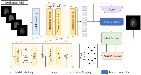
Figure 4. Model architecture
3.1 Model architecture
As depicted in Figure 4, brain tumor MRI is input into the image encoder via patch embedding, employing a Transformer architecture. To reduce the computational load required for model fine-tuning, the image encoder is frozen. The encoder contains multiple Transformer modules. Post-image encoder output, Transformer features are reshaped to $F_t \in \mathbb{R}^{C \times W \times H}$ through feature mapping. Subsequently, CNN features $F_c \in \mathbb{R}^{C \times W \times H}$ are obtained via three layers of 3*3 convolution operations. To better fuse local and global features, a FFB is utilized between CNN and Transformer features for feature fusion and correction, resulting in fused features with superior representational capabilities, thereby enhancing the precision of segmentation results. The mask decoder employs a Transformer decoding module, which upsamples the image tokens. An MLP maps the output tokens to a dynamic linear classifier, calculating the probability of the mask at prominent locations in the image.
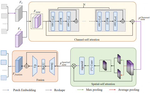
3.2 FFB
The FFB principally consists of three steps: channel self-attention, spatial sub-attention, and fusion, as illustrated in Figure 5.
Figure 5. FFB
Initially, combined features $F_{n e w} \in \mathbb{R}^{2 C \times W \times H}$ are obtained through aggregation of $F_t$ and $F_c$. The output $F_{n e w}^n \in \mathbb{R}^{2 C \times W \times H}$ from $F_{n e w}$ through the channel self-attention module can be derived using the following equation:
$\begin{aligned} & F_{n e w}^n =\oplus\left\lceil\operatorname{Conv}_{3 \times 3}\left(\operatorname{ReLU}\left(\operatorname{Conv}_{3 \times 3}\left(F_{n e w}^{n-1}\right)\right)\right), F_{n e w}^{n-1}\right\rceil\end{aligned}$ (1)
where, $n=\{1,2, \cdots, N\}$, and $N=4$. The channel self-attention feature can be calculated by the equation below:
$F_{\text {new }}^{\text {channel }}=\bigoplus\left(F_{\text {new }}, F_{\text {new }}^n\right)$ (2)
where, $\oplus$ represents element-wise addition, $\operatorname{Conv}_{3 \times 3}(\cdot)$ denotes the $3 * 3$ convolution operation, and $\operatorname{ReLU}(\cdot)$ signifies an activation function.
Upon obtaining the channel self-attention feature $F_{\text {new }}^{\text {channel }}$, it is reshaped and then inputted for spatial self-attention weighting. Through parallel operations of max and average pooling, $F_{\text {spatial }}^{\max }$ and $F_{\text {spatial }}^{\text {average }}$ are obtained from $F_{\text {new }}^{\text {channel }}$:
$F_{\text {spatial }}^{\max }=\operatorname{Maxpooling}\left(F_{\text {new }}^{\text {channel }}\right)$ (3)
$F_{\text {spatial }}^{\text {average }}=$ Averagepooling $\left(F_{\text {spatial }}^{\text {average }}\right)$ (4)
Subsequently, a 1*1 convolution is applied to both $F_{\text {spatial }}^{\max }$ and $F_{\text {spatial }}^{\text {average }}$. Through sigmoid operation, the spatially weighted feature map $F_{\text {map }}^{\text {Sweight }}$ is derived:
$F_{\text {map }}^{\text {sweight }}=\operatorname{Resape}\left[\sigma\left[\operatorname{Conv}_{1 \times 1}\left(\operatorname{concat}\left(F_{\text {spatial }}^{\text {max }}, F_{\text {spatial }}^{\text {average }}\right)\right)\right]\right]$ (5)
$F_{\text {map }}^{\text {Sweight }}$ is weighted to the spatial self-attention input feature to obtain spatially weighted features $F_{n e w}^{\text {spatial }}$, which can be calculated by the equation:
$F_{\text {new }}^{\text {spatial }}=\otimes\left[F_{\text {map }}^{\text {Sweight }}, F_{\text {new }}^{\text {channel }}\right]$ (6)
where, $\otimes$ represents element-wise multiplication, $\sigma(\cdot)$ denotes the sigmoid operation, and Maxpooling $(\cdot)$ and Averagepooling $(\cdot)$ signify max and average pooling, respectively.
Finally, for feature correction, the fusion module is used for the final adjustment. As input features for fusion, $F_{\text {new }}^{\text {spatial }} \in \mathbb{R}^{C \times W \times H}$ undergo a 1*1 convolution and max pooling for downsampling. After the ReLU activation, they are then upsampled through the 1*1 convolution and linear interpolation to restore feature resolution. $F_{\text {fusion }}$ can be obtained by the equation below:
$F_{\text {fusion }}=\oplus\left[U p\left(\operatorname{ReLU}\left(\operatorname{Down}\left(F_{\text {new }}^{\text {spatial }}\right)\right)\right), F_{\text {new }}^{\text {spatial }}\right]$ (7)
4.1 Dataset
The performance of the model was evaluated using the BraTS2021 dataset. BraTS2021 is a large-scale multimodal brain glioma MRI segmentation dataset comprising 2040 cases, including 1251 cases in the training set, 219 cases in the validation set, and the remainder in the test set. Each case contains four modalities: T1, T1ce, T2, and FLAIR, with each modality having dimensions of 240×240×155 (L×W×H). The annotations in BraTS2021 primarily include the ET, the ED, and the NCR.
Given that only the training set possesses actual segmentation masks, making it more suitable for the segmentation method used in this study, the model was evaluated using the training set. A single MRI sequence was used as the input to assess the accuracy of model segmentation. Since physicians are more concerned with the tumor core (TC) location in clinical treatment, the TC segmentation was examined on the contrast-enhanced T1-weighted sequence, considering the characteristics of each MRI modality.
4.2 Experimental process
The experimental setup was equipped with a workstation featuring 8 NVIDIA A100 GPU, running on Python 3.10.0, Pytorch 1.10.1, and CUDA 11.1 for local execution. The model was trained over 100 epochs. MRI voxel intensity was normalized to a range between 0 and 255 by dividing by the maximum intensity of each 3D dataset and subsequently multiplying by 255.
Specifically, MRI was divided into two-dimensional slices along the plane's outer dimension. A pre-trained ViT-B model encoder [19] was employed as the image encoder to compute all image embeddings. The AdamW optimizer (β1=0.9, β2=0.999) [20] was selected, with an initial learning rate set at 1e-5 and a weight decay of 0.1. A cosine annealing learning rate scheduler was used to adaptively decrease the maximum learning rate smoothly to a minimum value (1e-7).
Partial Encoder Fine-Tuning (PEFT) technique was applied for fine-tuning the model, keeping the encoder part (image and prompt encoders) parameters frozen and only updating the gradients of the decoder. This approach aims to enhance the model's performance with limited data and computational resources, reducing the number of parameters that needed to be optimized during training.
4.3 Evaluation metrics
To evaluate the accuracy of the segmentation model, the Dice Similarity Coefficient (DSC), Hausdorff Distance (HD), and Average Symmetric Surface Distance (ASSD) were employed as evaluation metrics.
The DSC measures the similarity between the predicted and true segmentation results. Similar to the IoU, its range is from 0 to 1, with 1 indicating the maximum similarity between prediction and truth. The DSC is calculated as follows:
$D S C=\frac{2|A \cap B|}{|A|+|B|}=\frac{2 T P}{2 T P+F P+F N}$ (8)
The HD first calculates the minimum distance from each point in set A to set B, and then selects the maximum value among these distances. To mitigate the influence of outliers, HD95 is the 95th percentile of all these distances. The HD is calculated using the formula below:
$h(A, B)=\max _{a \in A} \min _{b \in B} d(a, b)$ (9)
where, d(a,b) represents the distance between points a and b.
The ASSD is used to measure the degree of surface alignment in the segmentation results. It calculates the minimum distance from each point on the segmented surface to the ground truth surface, and vice versa, taking the average of these two sets of minimum distances. The smaller the value, the better the segmentation performance. The ASSD can be represented by the formula:
$\frac{1}{S(A)+S(B)}\left(\sum_{s_i \in S(A)} d\left(s_A, S(B)\right)+\sum_{s_B \in S(B)} d\left(s_B, S(A)\right)\right)$ (10)
where, S(A) denotes the surface voxels in set A, and d(v,S(A)) represents the shortest distance from any voxel to S(A).
4.4 Experimental results and analysis
This study evaluated the predictive accuracy of the model using three nested structures of the following subregions: ET, TC (ET + NCR + NET), and the whole tumor (WT) (i.e., TC + ED). The segmentation results of the U-net, Unet++, ResUnet, TransUnet, and SAM on the BraTS2021 dataset were compared. To contrast the interactive performance of SAM, segmentation of brain tumors was conducted using 2 prompt points, 10 prompt points, and a fully automatic segmentation approach. The segmentation results with 10 prompt points surpassed those with 2 prompt points, indicating that a greater number of prompt points leads to improved final segmentation outcomes.
Table 1. Comparison of model segmentation results
|
Method |
DSC |
HD |
ASSD |
||||||
|
ET |
TC |
WT |
ET |
TC |
WT |
ET |
TC |
WT |
|
|
U-net [21] |
0.7192 |
0.7768 |
0.8106 |
29.6654 |
19.8751 |
28.3322 |
2.8832 |
2.6702 |
2.6570 |
|
Unet++ [22] |
0.7015 |
0.7106 |
0.8009 |
27.9513 |
17.4712 |
27.7822 |
2.8832 |
2.6702 |
2.6570 |
|
ResUnet [23] |
0.7006 |
0.7841 |
0.7816 |
28.3260 |
19.9965 |
27.9957 |
2.6780 |
2.9053 |
2.7256 |
|
TransUNet [24] |
0.7439 |
0.7524 |
0.7860 |
27.1583 |
19.8313 |
28.1590 |
2.7792 |
2.6702 |
2.9205 |
|
SAM 2 point |
0.3211 |
0.4194 |
0.4164 |
22.4959 |
22.9007 |
27.9233 |
2.9952 |
2.5032 |
2.9362 |
|
SAM 10 point |
0.5199 |
0.6306 |
0.6453 |
16.470 |
16.3422 |
20.5195 |
2.7836 |
2.4395 |
2.5763 |
|
SAM (auto) |
0.5915 |
0.7285 |
0.6989 |
12.5408 |
13.2353 |
17.2557 |
1.2528 |
2.8809 |
3.1699 |
|
Our method (auto) |
0.7321 |
0.7503 |
0.8091 |
11.2536 |
18.1524 |
22.0658 |
1.1057 |
1.5216 |
1.1563 |
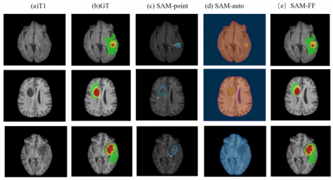
The results are displayed in Table 1. It is observed that the segmentation method of this study outperforms the original SAM prompt points and automatic segmentation methods in terms of segmentation effects, with DSC surpassing the best segmentation outcomes. SAM demonstrated the best segmentation effects on the TC, followed by the WT, and lastly the ET. This indicates that SAM exhibits superior performance on objects with clearer boundaries, as the TC has the clearest boundaries among the three regions. The model's best segmentation effects were observed in the WT region in Figure 6.
Figure 6. Visualization of segmentation results
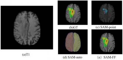
Figure 7 shows two heterogeneous tumor regions, more prompt points are needed, as demonstrated in this study, where 2 positive sample points and 3 negative sample points were utilized. However, the segmentation results for ET and ED were suboptimal.
Figure 7. Visualization of segmentation results of two heterogeneous tumor regions
The automatic segmentation of brain tumors is crucial for clinical diagnosis and treatment. This article adds convolution and feature mapping to the original architecture of SAM, allowing for the extraction of deeper image features. By fusing the convolved features with the Transformer features within the image encoder, precise segmentation of brain tumors has been achieved. Through experimental verification, the method proposed in this paper achieved better accuracy in brain tumor segmentation than the original SAM method. In addition, this study investigated the segmentation results of different numbers of SAM cue points, indicating that increasing the number of cue points helps improve segmentation results.
However, only T1 was validated in this article, without considering the contextual information of the slices. Therefore, future researchers can further explore the use of SAM for multimodal brain tumor segmentation, extending 2D segmentation results to 3D. This progress will help doctors diagnose and treat brain tumor patients before surgery.
[1] Havaei, M., Davy, A., Warde-Farley, D., Biard, A., Courville, A., Bengio, Y., Pal, C., Jodoin, P.M., Larochelle, H. (2015). Brain tumor segmentation with deep neural networks. Medical Image Analysis, 35: 18-31. https://doi.org/10.1016/j.media.2016.05.004
[2] Wadhwa, A. Bhardwaj, A., Verma, V.S. (2019). A review on brain tumor segmentation of MRI images. Magnetic Resonance Imaging, 61: 247-259. https://doi.org/10.1016/j.mri.2019.05.043
[3] Roy, S., Nag, S., Maitra, I.K., Bandyopadhyay, S.K. (2013). A review on automated brain tumor detection and segmentation from MRI of brain. https://doi.org/10.48550/arXiv.1312.6150
[4] Brown, T.B., Mann, B., Ryder, N., et al. (2020). Language models are few-shot learners. https://doi.org/10.48550/arXiv.2005.14165
[5] Kirillov, A., Mintun, E., Ravi, N., Mao, H., Rolland, C., Gustafson, L., Xiao, T., Whitehead, S., Berg, A.C., Lo, W.Y., Dollár, P., Girshick, R. (2023). Segment anything. In Proceedings of the IEEE/CVF International Conference on Computer Vision, Paris, France, pp. 4015-4026. https://doi.org/10.1109/ICCV51070.2023.00371
[6] Ding, L., Zhu, K., Peng, D., Tang, H., Yang, K., Bruzzone, L. (2024). Adapting segment anything model for change detection in VHR remote sensing images. IEEE Transactions on Geoscience and Remote Sensing. https://doi.org/10.1109/TGRS.2024.3368168
[7] Ahmadi, M., Lonbar, A. G., Sharifi, A., Beris, A.T., Nouri, M., Javidi, A.S. (2023). Application of segment anything model for civil infrastructure defect assessment. https://doi.org/10.48550/arXiv.2304.12600
[8] Bommasani, R., et al. (2021). On the opportunities and risks of foundation models. https://doi.org/10.48550/arXiv.2108.07258
[9] Bahdanau, D., Cho, K., Bengio, Y. (2014). Neural machine translation by jointly learning to align and translate. Computer Science. https://doi.org/10.48550/arXiv.1409.0473
[10] Ma, Z., Hong, X., Shangguan, Q. (2023). Can SAM count anything? An empirical study on SAM counting. https://doi.org/10.48550/arXiv.2304.10817
[11] Dai, H., Ma, C., Yan, Z.L., Liu, Z.L., Shi, E.Z., Li, Y.W., Shu, P., Wei, X.Z., Zhao, L., Wu, Z.H., Zeng, F., Zhu, D.J., Liu, W., Li, Q.Z., Sun, L.C., Zhang, S., Liu, T.M., Li, X. (2023). Samaug: Point prompt augmentation for segment anything model. https://doi.org/10.48550/arXiv.2307.01187
[12] Zhang, Z.Y., Cai, H., Han, S. (2024). EfficientViT-SAM: Accelerated segment anything model without performance loss. https://doi.org/10.48550/arXiv.2402.05008
[13] Song, Y., Zhou, Q., Li, X.T., Fan, D.P., Lu, X.Q., Ma, L.Z. (2024). BA-SAM: Scalable bias-mode attention mask for segment anything model. https://doi.org/10.48550/arXiv.2401.02317
[14] Rajič, F., Ke, L., Tai, Y.W., Tang, C.K., Danelljan, M., Yu, F. (2023). Segment anything meets point tracking. https://doi.org/10.48550/arXiv.2307.01197
[15] Zhang, P., Wang, Y.P. (2023). Segment anything model for brain tumor segmentation. https://doi.org/10.48550/arXiv.2309.08434
[16] Zhang, Y., Jiao, R. (2023). Towards segment anything model (SAM) for medical image segmentation: A survey. https://doi.org/10.48550/arXiv.2305.03678
[17] Mattjie, C., de Moura, L.V., Ravazio, R. C., Kupssinskü, L.S., Parraga, O., Delucis, M.M., Barros, R.C. (2023). Zero-shot performance of the Segment Anything Model (SAM) in 2D medical imaging: A comprehensive evaluation and practical guidelines. https://doi.org/10.48550/arXiv.2305.00109
[18] Hu, M.Z., Li, Y.H., Yang, X.F. (2023). SkinSAM: empowering skin cancer segmentation with segment anything model. https://doi.org/10.48550/arXiv.2304.13973
[19] Dosovitskiy, A., Beyer, L., Kolesnikov, A., Weissenborn, D., Zhai, X.H., Unterthiner, T., Dehghani, M., Minderer, M., Heigold, G., Gelly, S., Uszkoreit, J., Houlsby, N. (2020). An image is worth 16x16 words: Transformers for image recognition at scale. https://doi.org/10.48550/arXiv.2010.11929
[20] Loshchilov, I., Hutter, F. (2017). Decoupled weight decay regularization. https://doi.org/10.48550/arXiv.1711.05101
[21] Ronneberger, O., Fischer, P., Brox, T. (2015). U-net: Convolutional networks for biomedical image segmentation. In Medical Image Computing and Computer-Assisted Intervention–MICCAI 2015: 18th International Conference, Munich, Germany, pp. 234-241.
[22] Zhou, Z., Rahman Siddiquee, M.M., Tajbakhsh, N., Liang, J., (2018). Unet++: A nested u-net architecture for medical image segmentation. In Deep Learning in Medical Image Analysis and Multimodal Learning for Clinical Decision Support: 4th International Workshop, DLMIA 2018, and 8th International Workshop, ML-CDS 2018, Held in Conjunction with MICCAI 2018, Granada, Spain, pp. 3-11. https://doi.org/10.1007/978-3-030-00889-5_1
[23] Xiao, X., Lian, S., Luo, Z., Wang, S., Tang, J. (2018). Weighted Res-UNet for high-quality retina vessel segmentation. In 2018 9th International Conference on Information Technology in Medicine and Education (ITME), Hangzhou, China, pp. 474-478. https://doi.org/10.1109/ITME.2018.00080
[24] Chen, J., Lu, Y., Yu, Q., Luo, C., Adeli, E., Wang, Y., Lu, L., Yuille, A.L., Zhou, Y.Y. (2021). TransUNet: Transformers make strong encoders for medical image segmentation. https://doi.org/10.48550/arXiv.2102.04306