Dagada Madhu Sudhan Reddy*![]() | Usha Rani Neerugatti
| Usha Rani Neerugatti![]()
© 2023 IIETA. This article is published by IIETA and is licensed under the CC BY 4.0 license (http://creativecommons.org/licenses/by/4.0/).
OPEN ACCESS
Agriculture serves as the mainstay of India's economy, bearing a vital responsibility in nourishing an expanding populace. The thriving of this sector is contingent upon numerous variables, among which the choice of the optimal crop plays a pivotal role. The advent of Machine Learning (ML) has engendered a transformative impact on the agricultural sector by facilitating the prediction of suitable crops, contingent on soil attributes. This study undertakes the examination of diverse ML algorithms, encompassing Decision Tree, Linear Regression, Naïve Bayes, Random Forest, Extreme Gradient Boosting (XGBoost), and Support Vector Machine, to assess their efficacy in recommending optimal crops based on soil parameters. The parameters under consideration include Phosphorus, Nitrogen, Potassium, Electrical Conductivity, pH, Organic Carbon, Boron, Iron, Zinc, Copper, Manganese, and Sulphur. The crop recommendations are focused on Rice, Cotton, and Jowar for the Kurnool district of Andhra Pradesh, India. Among the assessed models, it was observed that the XGBoost model surpassed others in terms of accuracy in determining the most suitable crop for the given soil parameters. The experimental findings substantiate the precision of the model in forecasting the apt crop, thereby underscoring the immense potential of ML in the agricultural domain. This investigation signifies a considerable stride towards optimal crop recommendation, thereby increasing the potential for enhanced yield and profitability. Through the incorporation of technological innovation, agriculture can be rendered more efficient, cost-effective, and sustainable, thus laying the groundwork for a promising future.
machine learning, agriculture, XGBoost, decision tree, random forest, crop, recommendation, naïve bayes
In India, Agriculture plays a crucial role in the nation’s economy. More than 70% of rural families depend on agriculture. Agriculture has a big economical influence as it contributes 20% of the country's GDP. Kurnool is one of the districts of Andhra Pradesh, where the usual cultivated crops are Rice, Cotton, and Jowar. Agriculture is also additionally contributing to the development of diverse ancillary industries together with agricultural machinery, fertilizers, pesticides, garage centres, transportation, and agro-processing, and those industries contribute to the general economy through developing employment opportunities and riding economic boom. Indian agriculture has grown significantly during the last few decades. Since independence, food grain output has increased from 51 million tonnes to 149.92 million tonnes from the crop year 1950-1951 to 2022-23 and employs around 58% of the workforce. As the Indian population is 1.42 billion, agriculture still ensures food security for the nation.
Artificial Intelligence (AI) based agriculture enables Indian farmers to make precise decisions about irrigation, fertilization, and pest control by gathering real- time data on soil moisture, nutrient levels, crop health, etc. Recently, farmers initiated data- driven strategies to increase crop yields, resource conservation, and improved sustainability. Farmers can efficiently allocate resources, identify crop stress or diseases early, and make wise choices to increase productivity and profitability with the aid of AI and analytics. Indian farmers can improve their farming practices, reduce risks, and support the nation's sustainable agricultural growth by use of precision agriculture.
Artificial Intelligence (AI) is a cutting-edge and rapidly developing research area in the computer science domain. John McCarthy and his team coined the term “AI” at the Dartmouth Conference in 1956 [1], defining it as the science and engineering of creating intelligent machines. Machine Learning [2] (ML) is a leading sub-domain of AI. One of the American pioneers of the AI field, Arthur Samuel coined the term "Machine Learning" (ML) in the year 1959. It is defined as "a field of study that allows computers to learn without being explicitly programmed" [3].
ML is also revolutionizing Indian agriculture by enabling improved decision-making, market research, accuracy agriculture, disease detection, produce prediction, farm automation, and optimized crop management. Farmers of India can increase productivity, conservation, success, and support the expansion and development of the agricultural sector by utilizing ML.
The central idea of using an ML in the current work is to choose the best crop to be farmed. As the result, the outcomes are incredibly advantageous for agricultural growers. Along with high-performance computing and Big Data technologies, ML has arisen to provide new options for designing quality and effective data-driven models in agricultural work contexts. Research and development of ML applications in agriculture must be promoted. Several application areas of ML are introduced, such as automated irrigation systems [4], agricultural drones for field analysis [5], crop monitoring systems [6], precision agriculture [7], animal identification, etc. To make crop recommendations, agricultural experts often use sophisticated modelling software that takes into a different range of variables, such as precipitation patterns, soil types, rainfall and temperature. The models use historical data to estimate yields and suggest the best crops to plant for the upcoming season. Farmers can also use online tools and mobile applications to receive crop recommendations. These tools often require farmers to input information about their land, including soil type, climate, and previous crop yields. So that farmers can be benefitted by using Machine Learning.
Crop selection is the first and important step of crop cultivation cycle. Different approaches have following to select right crop. Literature work classified based on models used by authors. Such Machine Learning based models, Deep Learning based models, other approaches.
2.1 Machine learning techniques
To recommend the appropriate crop, several machine learning models [8] predict suitable crop based on soil series with regard to land. For soil classification, a number of machine learning techniques are utilised, including weighted K-Nearest Neighbour (KNN), Support Vector Machines (SVM) model with help of Gaussian kernel, and bagged trees. It selected the crop by analyse soil type, instead of soil properties and accuracy can be improved.
And SVM-based technique outperforms many other models, according to experimental results. An ensemble model [9] recommends the crop based on a majority count technique that uses Naive Bayes, Random Tree, KNN, and Chi-squared Automatic Interaction Detection (CHAID) as learners to accurately for the site-oriented parameters, and the better result given by Naive Bayes with 88%. Here model recommended the crop just based on soil pH, water holding, drainage, and texture.
A crop-suggested system [10] helps farmers select crops by considering into account all the variables like planting season, soil, and geographic location. Furthermore, precision agriculture, which focuses on site-specific crop management, by taking models Decision Tree (DT), K-Nearest Neighbors (KNN), KNN with cross-validation, Logistic Regression (LR), Naïve Bayes, and Neural Network (NN). The NN had given better accuracy with 89.88%. But implementation of NN is complex task.
A classification technique, an extreme learning machine to suggest the best crop [11] to farmers based on considering various significant factors, soil fertility, soil condition, and season. It also determines whether the soil has insufficient nutrients for the needs of the current crop, the model also contains a deficiency analysis. The results of the experimental analysis showed that the suggested model is more accurate in forecasting suitable crops and identifying soil deficiencies, with a minimal false-positive rate of 3.5% and an average accuracy of roughly 96.5%. It recommends the crop by considered mainly on crop rotation.
A unique ML-powered crop recommendation tool [12] with cloud support to find the best suitable crop based on input data. It is providing precision farming-based solutions that are open source and free and will promote the adoption and growth of precision farming solutions. It also compares predictive ML algorithms such as K-Nearest Neighbours (KNN), Random Forest (RF), Decision Tree (DT), and Support Vector Machine (SVM). Accuracy can be improved by changing hyperparameters such as the maximum depth of the random forest.
A model includes abstract and theoretical [13] of a recommendation system for crop selection by integrating models of collecting environmental factors using Arduino microcontrollers, ML techniques such as Multinomial Nave Bayes, SVM, K- Means clustering and Natural Language Processing. It has been delicate to determine what to grow, as any man has sufficient framing land.
Random Forest, Linear SVM, and Naive Bayes serve as ensemble-based models [14]. Every classifier offers a unique set of class labels with a respectable level of accuracy. The majority voting method is used to integrate the class labels of distinct base learners. The input soil dataset is divided into two categories by the recommendation system for crops: Rabi and Kharif. The dataset includes samples of the average rainfall and surface temperature as well as the physical and chemical properties particular to the soil. The model gave good classification accuracy, only when the independent base learners are combined.
2.2 Deep learning techniques
A crop-specific recommender system [15] based on Deep Learning Technique (DLT) compiled historical information on crops and climate. To optimise the inputs to Deep Convolution Neural Networks (DCCN) and Long Short Term Memory (LSTM) networks for crop predictions, a hybrid technique named Ant Colony Optimization along with DCNN, LSTM (ACO-IDCNN-LSTM) has been proposed. DCNNs often produce excellent levels of accuracy, but the number of processing layers increases the computational complexity. Since adding weights to DCNNs' nodes makes up a significant portion of complexity increases, it modifies these weights during training to simplify processing. For DCNN predictions on crops and to assist simplify weights, ACOs optimize hyperparameters during training. Although it is quite complex to implement as CNN, LSTM were used in the model. And the convergence rate of ACO is high.
2.3 Other techniques
Another crop-selection model [16] was developed by considering weight calculation, categorization, and prediction. 27 input criteria were divided into 7 major categories: water (2 sub-criteria), soil (11 sub-criteria), facilities (3 sub-criteria), risk (2 sub-criteria), input (6 sub-criteria), season (no sub-criteria), and support (2 sub-criteria). In the suggested model, the relative weights of each main criterion's sub-criteria were determined using the rough set methodology, and the relative weights of the main criteria themselves were derived using the method called Shannon's Entropy. The ranking index of the primary criteria in this study was determined using the VIKOR (VIseKriterijumska Optimizacija I Kompromisno Resenje) approach since it is Multicriteria Optimization and Compromise Solution and efficient at sorting the alternatives. The outputs of the rough set method, Shannon's Entropy method, and the VIKOR method were combined to create a soft decision system. Too many parameters are involved to recommend a crop the and model is required more knowledge to understand.
Based on normal observations and the Mahalanobis distance, a multiclass model [17] developed using the Improved Mahalanobis Taguchi System (IMTS) uses distance measurement, which can be applied to agricultural development. The total input factors are twenty-six, which are important to crop cultivation were found and were grouped into six main factors for the creation of the model. The multiclass classification model is created with the relative importance of factors to improve significantly. Three crops are classified by an objective function is defined, those are paddy, groundnut, and sugarcane. No feature selection methods were used to find the best features among the total features.
A crop recommends by the suggested system [18] aids farmers in choosing the best crop for the season and sowing area by using Pattern Matching. The farmers will benefit as a result since their net profit will increase. The system can recommend a list of crops that is most beneficial for farmers in their selection by taking into account multiple datasets, which mainly contain five criteria: soil moisture, rainfall, rainfall humidity, slope, and temperature data values belonging to horticulture. Pattern Matching may not be suitable when soil parameters vary from one farmland to another land.
Another Graphic User Interface (GUI) supported crop prediction model [19] was created in the Flask environment using the Map-Reduce method. It provides the environment, where input can be given and suggested crops can be displayed on the user’s screen. Soil moisture, irrigation, cloud cover etc. can be included in the dataset to make the system effective.
A mobile app with Graphic User Interface (GUI) based crop suggestion model [20] recommends the crop based on input parameters of soil and weather data.
The Crop Selection Method [21] (CSM) proposed to solve the problem of crop selection, along with maximising the season’s crop net yield and gaining maximum economic improvement for the nation. This method increases the crop net yield rate. Soil characteristics are ignored by the method to select method, though it is an important parameter.
To predict crops using classification approaches that indicate the best crop(s) for the area, comparative research [22] of several wrapper feature selection methods is conducted. According to the experimental findings, the Adaptive Bagging classifier combined with the Recursive Feature Elimination method performs better than the others. This method’s accuracy can be improved by fine-tuning hyper-parameters of machine learning models.
The majority of existing literature works used non-tree-based machine learning models such as KNN, CHAID, LR, NB, NN, and Pattern Matching although ugh output is labelled class.
3.1 Dataset description
In the current work, a dataset is collected for the Kurnool district of Andhra Pradesh state. This dataset was gathered from a government website [23]. Before using it in the models, it needs to be pre-processed to avoid duplicate and outlier values that can create problems to learn by ML models. The dataset has a total of 67,788 data records for three crops Rice Cotton, and Jowar with 12 columns, and 5,649 rows. In the dataset, all features are about values of soil nutrients, which are Phosphorus (P), Nitrogen (N), Potassium (K), Electrical Conductivity (EC), pH, Organic Carbon (OC), Boron (B), Iron (Fe), Zinc (Zn), Copper (Cu), Manganese (Mn), and Sulphur (S).
3.2 Machine learning models
In general, there are two kinds of supervised learning models, one is Regression-based models, where predicted output is a continuous value. Decision Trees, Random Forest, Linear Regression, and Logistic Regression are a few examples of regularly used regression models. And second is Classifiers, where output is a discrete labelled value [24], which give based on input data. Support Vector Machine, Decision Trees, Logistic Regression, and Random Forest are a few examples of classifiers.
Performance metrics [25, 26] for classification models and also considered in existing literature research work are Accuracy, Precision, Recall, and F1 Score. These performance metrics evaluated how best the model performed for given data.
Accuracy is used to determine the efficiency of the model, which is based on the accurate predicted samples and total samples. In general, an accuracy rating shows if a version is being trained well and the way the model handles out in general.
Accuracy=(TP+TN)/(TP+FP+FN+TN)
where, TP-True Positives means positive classes that are also correctly predicted as positive. FP-False Positives means negative classes that are false predicted as positive. TN-True Negatives means negative classes that are correctly predicted as negative. FN-False Negatives means positive classes that are falsely predicted as negative.
Precision=TP/(TP+FP)
The precision score, which shows the proportion of accurately predicted positive observations to all expected positive observations, measures the classifier's differential rate.
Recall=TP/(TP+FN)
Recall measures the score which measures the rate of TP over the total number of true. In simple terms it measures the observations of predicted positive accurately and all in the actual class.
F1=(2×Precision×Recall)/(Precision+Recall)
The F1 score is an overall accuracy performance metric that combines both precision and recall. A solid F1 score suggested that there are few FPs and few FNs, and that mislead the classification process.
3.2.1 Naive bayes classifier
The Naive Bayes (NB) algorithm [27] is a simple supervised learning algorithm that makes use of Bayes' rule along with the strong assumption that the attributes are conditionally independent for a given class. NB often produces good classification accuracy by taking the fact that the independence assumption is frequently violated in practice. The NB [28] classifier is a fundamental conditional probability-based method that can predict the class which belongs among given classes. It may easily accommodate the missing attribute values by simply considering relevant probabilities for those characteristics when calculating the likelihood of membership for each class.
The simple form of Baye's rule is as follows:
$P(X \mid Y)=\frac{P(Y \mid X) \times P(X)}{P(Y)}$ (1)
where, P(Y|X) is a likelihood probability. It is the evidence when the hypothesis is true, P(X) is the prior probability and, P(Y) is the marginal probability. P(X|Y) is called the posterior probability of ‘X’ with given ‘Y’.
Naive Bayes classifier uses above Bayes' theorem to make predictions by assuming that the features are conditionally independent of given the set of features ‘X’. It calculates the posterior probability of each feature of ‘X’ and assigns the instance to the class with the highest probability. The formula for the Naive Bayes classifier is:
$P(C \mid X)=\frac{P(X \mid C) \times P(C)}{P(X)}$ (2)
where, P(C|X) is the posterior probability of class C given the feature vector X. P(X|C) is the likelihood probability of the feature vector X given class C. P(C) is the prior probability of class C. P(X) is the prior probability of the feature vector X.
Implement NB on taking dataset with different sizes of training and testing. The results are mentioned in Table 1.
Table 1. Prediction of accuracy by NB model
|
Size of Train-Test Data |
60-40 |
65-35 |
70-30 |
75-25 |
80-20 |
85-15 |
90-10 |
|
Accuracy in % |
53.8 |
52.2 |
52.1 |
53.7 |
58.4 |
53.6 |
54.5 |
As the training size is 60% and the testing size is 40%, NB has given an accuracy of 53.8%. And better result, 58.4% has given with 80-20 training and testing data sizes.
It gives prediction results based on probability of each feature and class. In this work, it gave moderate accuracy because of features of taken dataset are dependent.
3.2.2 Logistic regression classifier
Another model for classifying data is Logistic Regression [29] (LR). Typically, Logistic Regression uses the activation function, also known as the sigmoid function, to estimate the probabilities.
$f(z)=\frac{1}{1+e^{-z}}$ (3)
The above Eq. (2) is the formula of a sigmoid function f and e≈2.71 is the base of the natural logarithm. The logistic regression hypothesis suggests that the function be restricted to the range of 0 and 1.
For multi-class classification Logistic Regression classifier uses above Eq. (2) with “One-vs-All” (OvA). A multi-class classification problem with K classes, the logistic regression model will create K separate binary classifiers, each trained to distinguish one class from the rest.
For a given instance with a feature vector X, the OvA strategy involves calculating the probability of it belonging to each class and selecting the class with the highest probability.
The formula for the OvA logistic regression model is:
$\boldsymbol{P}(\boldsymbol{y}=\boldsymbol{i} \mid \boldsymbol{X})=\operatorname{sigmoid}\left(\mathrm{w}_{\mathrm{i}} * X\right)$ (4)
where, P(y=i|X) is the probability of the instance belonging to class i given the feature vector X. sigmoid() is the logistic sigmoid function that maps the linear combination to a value between 0 and 1. wi is the weight vector associated with class i. X is the feature vector.
The weight vector wi represents the coefficients learned for class i. Each class has its own set of weight coefficients, and the model calculates the dot product between the weight vector and the feature vector to obtain the linear combination. The sigmoid function is then applied to transform the linear combination into a probability value.
For a dataset, this particular classifier evaluates the correlation between the categorical variable which are dependent and one or more independent variables. The target class is the dependent variable that will make a prediction. The attributes or features, on the other hand, are the independent variables that are utilised to forecast the target class. Simply said, logistic regression is an S-shaped curve that can take any number with a real value and convert it to a number between 0 and 1. The following formula carries out that mapping:
f(xi)= β0+ β1xi1+…+βpxip (5)
here β0, β1, ... βp are the regression coefficients. And here, xij denotes the values of jth feature of ith observation. To find the likelihood of f(x), apply cost function with respect to equation (3). Later gradient descent optimization needs to apply to find the optimal values of the hyperparameter of logistic regression.
Implement LR on taking dataset with different sizes of training and testing. The results are mentioned in Table 2.
Table 2. Prediction of accuracy by LR model
|
Size of Train-Test Data |
60-40 |
65-35 |
70-30 |
75-25 |
80-20 |
85-15 |
90-10 |
|
Accuracy in % |
60.0 |
62.0 |
60.6 |
59.1 |
64.1 |
60.2 |
62.1 |
As the training size is 60% and the testing size is 40%, LR has given an accuracy of 60.0%. It is a better result, when compared with NB. As features are dependent, sigmoid function curve classify data values.
3.2.3 Support vector machines classifier
Another well-known classification method often used for predictive analytics is Support Vector Machine [30] (SVM). Data variables of data space are often separated according to a class, either class 0 or class 1, using SVM as a binary classifier. To achieve this, the hyperplane of the vector machine is chosen as a line capable of traversing variable space. SVM seeks a line that optimises the separation between a two-class data set of two-dimensional space points in its simplest form, known as linear separation. Finding a hyperplane in n-dimensional space that optimises the separation of the data points to their prospective classes is the goal to generalise.
Support Vectors are the data points that are close to the hyperplane and have the smallest distance from it. Data point separation computations are based on a kernel function. Different kernel functions include linear, polynomial, Radial Basis Function (RBF), Gaussian, and sigmoid functions. Simply said, these functions govern the smoothness and efficiency of class separation, and tinkering with their hyperparameters might result in overfitting or underfitting.
Implement SVM on the dataset with different sizes of training and testing. The results are mentioned in Table 3.
Table 3. Prediction of accuracy by SVM model
|
Size of Train-Test Data |
60-40 |
65-35 |
70-30 |
75-25 |
80-20 |
85-15 |
90-10 |
|
Accuracy in % |
42.7 |
43.0 |
42.8 |
41.4 |
42.5 |
42.4 |
44.2 |
As the training size is 60% and the testing size is 40%, SVM has given an accuracy of 42.7%. Prediction rate of SVM is low due to generated hyperplanes are linear and not handled few outliers of data values.
3.2.4 Decision tree classifier
One of the most used methods for classification models is the use of Decision Trees [31] (DT). The study of DT has been growing by researchers in a variety of fields, including pattern recognition, statistics, machine learning, and data mining. It follows top-down strategies for building decision tree classifiers based on the data provided by the user. In Decision Tree, several splitting criteria such as Information Gain, Gene Index and pruning approaches as well as mathematical framework followed to make DT more effective. A basic algorithm proposed by Quinlan to create decision trees called ID3 (Iterative Dichotomiser 3).
The ID3 algorithm builds a DT using a top-to-bottom approach, where a greedy search through a given training data tree tests each attribute or context at each node. Information Gain has been calculated with the help of entropy, a statistical property used to select the attribute to be tested at each node in the tree. Quinlan proposes an extension based on the ID3 algorithm, namely the C4.5 algorithms. C4.5 builds a decision tree from the training dataset in the same way as ID3 with extra features like handling missing values and predicting continuous values. Paper [32] compared ID3/C4.5, C4.5/C5.0, and C5.0/CART with a dataset, which allowed and confirmed that C4.5 is unquestionably the most effective decision tree-based model.
A decision Tree is generated by splitting the root of the tree into two halves, which are split further by use of Entropy (E), and Information Gain (IG).
$\mathrm{E}=-\sum_{i=0}^n p_i * \log _2 p_i$ (6)
where, pi is the probability of selecting an example in class i.
Information Gain of current node S, with selected feature X is:
$I G(S, X)=E(S)-E(S, X)$ (7)
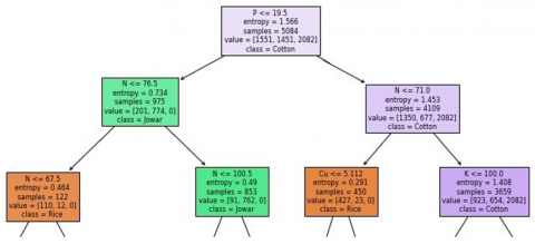
The highest IG of all features is selected as the root node of the decision tree, then sub-trees are formed. Repeat the process till all features are covered in the decision tree as leaves or sub-root. For current work, the below decision tree is formed.
Figure 1 shows that the splitting of the decision tree started with the feature “P” (P <= 19.5), followed by “N”, “Cu”, “K”, etc, towards the bottom of the tree. At last, it had shown a suitable crop based on traversed tree feature values.
Implement DT on the dataset with different sizes of training and testing. The results are mentioned in Table 4.
Table 4. Prediction of accuracy by DT model
|
Size of Train-Test Data |
60-40 |
65-35 |
70-30 |
75-25 |
80-20 |
85-15 |
90-10 |
|
Accuracy in % |
70.7 |
70.9 |
71.2 |
71.1 |
71.2 |
70.4 |
72.0 |
As the training size is 60% and the testing size is 40%, DT has given an accuracy of 70.7%. Better result, 72.0% has given with 90-10 training and testing data sizes. It has given better accuracy than SVM because DT splits the root of the tree based on the high IG feature of the feature set.
The DT is generated for the dataset. The root of DT is “P”. The top portion of DT is mentioned in Figure 1. The main hyperparameters of the DT are {'criterion': 'entropy', 'max_depth': 5, 'min_samples_leaf': 1, 'min_samples_split': 2, 'splitter': 'best'}
For soil parameters, N, P, K, pH, EC, OC, B, Zn, Fe, Mn, Cu, and S are 31.0,560.0, 7.42, 0.4, 0.39, 1.570, 11.42, and 25.480, DT predicted as “Rice”.
3.2.5 Random forest classifier
A Random Forest (RF) classifier is a type of ensemble machine learning method that considers multiple parallel Decision Tree algorithms together and provides a predictive result. A Random Forest [33] combines bootstrap assembly (sacking) and random feature selection to form a collection of decision trees with a controlled variation. Generate multiple decision trees for a given data set, it can reduce the cause of the single decision tree overfitting problem. In general, the random forest generates multiple decision trees instead of a single decision tree to predict the final activity class of output and consider the majority voting as the final result.
Implement RF on the dataset with different sizes of training and testing. The results are mentioned in Table 5.
Table 5. Prediction of accuracy by RF model
|
Size of Train-Test Data |
60-40 |
65-35 |
70-30 |
75-25 |
80-20 |
85-15 |
90-10 |
|
Accuracy in % |
78.5 |
80.0 |
79.7 |
80.9 |
83.0 |
80.8 |
81.9 |
As the training size is 60% and the testing size is 40%, RF has given an accuracy of 78.5%. Better result, 81.9% has given with 90-10 training and testing data sizes. RF is better than DT because of more depth in the tree and bagging technique, which leads to better classification.
An alternative to Information Gain is the Gini index.
Gini index $=1-\sum_{i=1}^j P(i)^2$ (8)
where, j represents the no. of classes in the target variable, P(i) represents the ratio of Pass/Total no. of observations in node. The Gini index gives information on the impurity of all features. Based on that root of the tree can be split into subtrees. For current the work, the below random tree is formed by considering gini index.
The RF is generated for the dataset. The root of RF is “N”. The top portion of RF is mentioned in Figure 2. The main hyperparameters of the RF are {'bootstrap': True, 'criterion': 'gini', 'max_depth': None, 'max_features': 'sqrt', 'min_samples_leaf': 1, 'min_samples_split': 2, 'n_estimators': 20}.
Figure 1. Decision Tree model for crop prediction (feature splitting)
Figure 2. Random forest model for crop prediction (feature splitting)
The RF, features of data splitting start with “N”, “Fe”, “S” etc., for example, if “N” is less than 70.5, then consider the left sub tree which is further classified based on “Fe” value, if “Fe” is less than 9.627, repeat the same above process, and last consider class is an output of classification.
For example, N, P, K, pH, EC, OC, B, Zn, Fe, Mn, Cu, and S are 88.0, 73.0, 368.0, 8.53, 0.09, 0.85, 2.280, 0.434, 21.340, 6.690, 21, 340, 11.0, then predicted by RF is class “Cotton”.
3.2.6 Extreme gradient boost classifier
The gradient-boosted decision trees have an extension known as XGBoost, which was first proposed by Tianqi Chenin in the paper [34]. The gradient-boosted trees approach is one of the most used and well-implemented in form of a decision tree. The XGBoost tree structure is shown in Figure 3 [35-37].
It should be observed that the residual of tree-1(weak tree) is supplied to tree-2(another weak tree) to lower the residue, and this process is repeated till the last tree-n. Unlike Random Forest, every tree model of XGBoost reduces the residual from the tree model before it. Just the first-order derivative of error information is used by the classic Gradient Boosted Decision Trees (GBDT). XGBoost employs both the first and second-order derivatives to perform cost functions. Moreover, the XGBoost tool enables the configurable cost function. Gradient boosting, combines the predictions of several weak trees, and simpler models to attempt to predict a target variable properly. For regression, gradient boosting is considered weak trees and associates each input data point with a leaf that holds a continuous score.
Figure 3. Simplified structure of extreme gradient boosting (XGBoost)
Using a convex loss function and a penalty term for model complexity, XGBoost [36] minimises a regularised (L1 and L2) objective function. It has been used to address a variety of classification issues in numerous domains. Iterative training is a process used to create the next level of new trees that predict the residuals or mistakes of previously generated trees, which are then incorporated with previous trees to produce the final prediction. Gradient Boosting follows the process of gradient descent approach to minimise loss level by level when adding new models to make the model effective.
$\hat{\mathrm{y}}_i=\sum_{k=1}^K f_k\left(x_i\right)$ (9)
where, ŷ is the predicted value. Σk represents the summation over all weak trees. fk(x) is the prediction of the k-th weak tree for the input feature vector x.
The prediction of each weak learner is weighted by a learning rate (η) to control the contribution of that weak learner to the final prediction. Objective function for XGBoost is:
$\operatorname{obj}(\theta)=\sum_i^n l\left(y_i, \hat{y}_i\right)+\sum_k^K \Omega\left(\mathrm{f}_k\right)$ (10)
here, first term represents the loss function to be calculated for each iteration from i to n. And yi is actual value, ŷi is predicted value. And the second term represents the regularization parameter with respective function fk. Then, instead of learning the entire tree at once which makes the optimization harder, so the additive strategy, minimize the loss what it has learned and add a new tree which can be follow the same.
Implement XGBoost on taking dataset with different sizes of training and testing. The results are mentioned in Table 6.
Table 6. Prediction of accuracy by XGBoost model
|
Size of Train-Test Data |
60-40 |
65-35 |
70-30 |
75-25 |
80-20 |
85-15 |
90-10 |
|
Accuracy in % |
91.9 |
92.8 |
92.2 |
92.2 |
92.9 |
92.5 |
93.2 |
As the training size is 60% and the testing size is 40%, XGBoost has given an accuracy of 91.9%. Better result, 93.2% has given training and testing data sizes of 90-10, because residual errors of one tree are taken by the next tree and minimize error rate and continue the process till getting better accuracy. For that, XGBoost has hyperparameters maximum depth, learning rate, and number of the tree reducing the error rate.
The XGBoost is generated for the dataset. The root of XGBoost is “N”. The top portion of XGBoost is mentioned in Figure 3. Main hyperparameters of the XGBoost are {'objective': 'multi:softprob', 'learning_rate': None, 'max_depth': None,'subsample': None}.
Figure 4. XGBoost model for crop prediction (feature splitting)
Figure 4 shows the splitting of the tree starting with the feature “N< 70.5”, followed by “K<97”, “Cu<5.11”, “P”, etc, towards the bottom of the tree. At last, it has shown a suitable crop based on traversed tree feature values.
For soil parameters, N, P, K, pH, EC, OC, B, Zn, Fe, Mn, Cu, and S are 31.0,560.0, 7.42, 0.4, 0.39, 1.570, 11.42, and 25.480, then predicted by XGBoost is class “Rice”.
The dataset is divided into two parts – the training set and the testing set. The size of these sets can be different to allow for better learning by the models. For example, a size of 60-40 would mean that the training set takes sixty per cent of the total data while the testing set occupies forty per cent of the total data. Different sizes are taken in similar forms 65-35, 70-30, 75-25, 80-20, 85-15 and 90-10. Results of all models for different sizes of train-test data are taken in Table 7.
Tree-based models such as DT, RF, and XGBoost have given better performance when compared to non-tree-based models because of Naïve Bayes generated probability values for each feature of the class, which leads to predict targets with less accuracy. Support Vector Machine is expected well-balanced data to classify data values by using hyperplanes to give better results. And Logistic Regression gives less accuracy because the features of this dataset are dependent.
Table 7. Prediction of accuracy by each model in percentage with different sizes of train and test set
|
Different Size of Train-Test Data |
Machine Learning Models Accuracy in % |
|||||
|
DT |
NB |
SVM |
LR |
RF |
XGB |
|
|
60-40 |
70.7 |
53.8 |
42.7 |
60.0 |
78.5 |
91.9 |
|
65-35 |
70.9 |
52.2 |
43.0 |
62.0 |
80.0 |
92.8 |
|
70-30 |
71.2 |
52.1 |
42.8 |
60.6 |
79.7 |
92.2 |
|
75-25 |
71.1 |
53.7 |
41.4 |
59.1 |
80.9 |
92.2 |
|
80-20 |
71.2 |
58.4 |
42.5 |
64.1 |
83.0 |
92.9 |
|
85-15 |
70.4 |
53.6 |
42.4 |
60.2 |
80.8 |
92.5 |
|
90-10 |
72.0 |
54.5 |
44.2 |
62.1 |
81.9 |
93.2 |
Figure 5. Prediction of accuracy by each model in percentage with different sizes of the test set
Figure 5 is a graph representation of all models and all training and testing sizes. It shows that XGBoost has given more accuracy than the other models used at each testing ratio. By taking, all testing set into account to check the better accuracy of all ML models.
To determine the best model among DT, SVM, NB, LR, RF, and XGBoost, the best F1 score from each model must be taken into account to analyse in Table 8.
Table 8. F1 score of each model in percentage
|
S.No |
Model |
F1 Score in % |
|
1 |
Decision Tree |
69.3 |
|
2 |
Naive Bayes |
50.6 |
|
3 |
SVM |
27.5 |
|
4 |
Logistic Regression |
57.0 |
|
5 |
Random Forest |
79.0 |
|
6 |
XGBoost |
91.6 |
Figure 6. Accuracy comparison of ML models
From Table 8, it clearly shown XGBoost has given highest F1 score 91.6%. Here also, XGBoost has outperform over remain models.
The Figure 6 has considered best prediction accuracy of each model and it clearly shows that XGBoost is outperformed other models such as DT, SVM, NB, LR, and RF.
Compare to remain models, XGBoost has capability of fast regularization, parallelized across clusters through a combination of data parallelism, which is the process of multiplying a dataset by multiple subsets and distributing them to different machines simultaneously and model parallelism, which is when split a single tree among several machines or nodes.
Agriculture is an essential sector of the food supply and contributes to the country's GDP. Selecting the right crop is critical to increase yield and maximize profits for farmers. Suitable crop can recommend by Machine Learning to simplified this process, making it more efficient and effective. In this study, Support Vector Machines, Logistic Regression, Random Forest, Decision Trees, Naive Bayes, and XGBoost models were analysed to recommend the best crop to given farmer input soil characteristics. XGBoost emerged as the most accurate model, with an impressive accuracy score of 93.2%, surpassing the other Machine Learning models. This research highlights the potential of Machine Learning in agriculture, providing a promising avenue for farmers to make decision effective and achieve higher yields. By leveraging Machine Learning, it can create a sustainable food supply while driving economic growth, making agriculture a more efficient and profitable industry.
[1] Crevier, D. (1993). AI: The tumultuous history of the search for artificial intelligence. BasicBooks.
[2] Song, Y.Y., Lu, Y. (1997). Decision tree methods: Applications for classification and prediction. Shanghai Archives of Psychiatry, 27(2): 130-135. http://dx.doi.org/10.11919/j.issn.1002-0829.215044
[3] Muñoz, A. (2012). Machine learning and optimization. https://cims.nyu.edu/~munoz/files/ml_optimization.pdf.
[4] Vij, A., Vijendra, S., Jain, A., Bajaj, S., Bassi, A., Sharma, A. (2020). IoT and machine learning approaches for automation of farm irrigation system. Procedia Computer Science, 167: 1250-1257. https://doi.org/10.1016/j.procs.2020.03.440
[5] El Hoummaidi, L., Larabi, A., Alam, K. (2021). Using unmanned aerial systems and deep learning for agriculture mapping in Dubai. Heliyon, 7(10): e08154.
[6] Benos, L., Tagarakis, A.C., Dolias, G., Berruto, R., Kateris, D., Bochtis, D. (2021). Machine learning in agriculture: A comprehensive updated review. Sensors, 21(11): 3758. https://doi.org/10.3390/s21113758
[7] Hakkim, V.A., Joseph, E.A., Gokul, A.A., Mufeedha, K. (2016). Precision farming: the future of Indian agriculture. Journal of Applied Biology and Biotechnology, 4(6): 068-072. https://doi.org/10.7324/JABB.2016.40609
[8] Rahman, S.A.Z., Mitra, K.C., Islam, S.M. (2018). Soil classification using machine learning methods and crop suggestion based on soil series. In 2018 21st International Conference of Computer and Information Technology (ICCIT), pp. 1-4. https://doi.org/10.1109/ICCITECHN.2018.8631943
[9] Pudumalar, S., Ramanujam, E., Rajashree, R.H., Kavya, C., Kiruthika, T., Nisha, J. (2017). Crop recommendation system for precision agriculture. In 2016 Eighth International Conference on Advanced Computing (ICoAC), pp. 32-36. https://doi.org/10.1109/ICoAC.2017.7951740
[10] Priyadharshini, A., Chakraborty, S., Kumar, A., Pooniwala, O.R. (2021). Intelligent crop recommendation system using machine learning. In 2021 5th international conference on computing methodologies and communication (ICCMC), pp. 843-848. https://doi.org/10.1109/ICCMC51019.2021.9418375
[11] Murugesan, G., Radha, B. (2022). Crop rotation based crop recommendation system with soil deficiency analysis through extreme learning machine. International Journal of Engineering Trends and Technology, 70(4): 122-134. https://doi.org/10.14445/22315381/IJETT-V70I4P210
[12] Thilakarathne, N.N., Bakar, M.S.A., Abas, P.E., Yassin, H. (2022). A cloud enabled crop recommendation platform for machine learning-driven precision farming. Sensors, 22(16): 6299. https://doi.org/10.3390/s22166299
[13] Bandara, P., Weerasooriya, T., Ruchirawya, T., Nanayakkara, W., Dimantha, M., Pabasara, M. (2020). Crop recommendation system. International Journal of Computer Applications, 975: 8887.
[14] Kulkarni, N.H., Srinivasan, G.N., Sagar, B.M., Cauvery, N.K. (2018). Improving crop productivity through a crop recommendation system using ensembling technique. In 2018 3rd International Conference on Computational Systems and Information Technology for Sustainable Solutions (CSITSS), pp. 114-119. https://doi.org/10.1109/CSITSS.2018.8768790
[15] Mythili, K., Rangaraj, R. (2021). Crop recommendation for better crop yield for precision agriculture using ant colony optimization with deep learning method. Annals of the Romanian Society for Cell Biology, 4783-4794.
[16] Deepa, N., Ganesan, K. (2018). Multi-class classification using hybrid soft decision model for agriculture crop selection. Neural Computing and Applications, 30: 1025-1038. https://doi.org/10.1007/s00521-016-2749-y
[17] Deepa, N., Khan, M.Z., Prabadevi, B., PM, D.R.V., Maddikunta, P.K.R., Gadekallu, T.R. (2020). Multiclass model for agriculture development using multivariate statistical method. IEEE Access, 8: 183749-183758. https://doi.org/10.1109/ACCESS.2020.3028595
[18] Kedlaya, A., Sana, A., Bhat, B.A., Kumar, S., Bhat, N. (2021). An efficient algorithm for predicting crop using historical data and pattern matching technique. Global Transitions Proceedings, 2(2): 294-298. https://doi.org/10.1016/j.gltp.2021.08.060
[19] Gupta, R., Sharma, A.K., Garg, O., Modi, K., Kasim, S., Baharum, Z., Mahdin, H., Mostafa, S.A. (2021). WB-CPI: Weather based crop prediction in India using big data analytics. IEEE Access, 9: 137869-137885. https://doi.org/10.1109/ACCESS.2021.3117247
[20] Usha Rani, N., Gowthami, G. (2020). Smart Crop Suggester. In: Jyothi, S., Mamatha, D., Satapathy, S., Raju, K., Favorskaya, M. (eds) Advances in Computational and Bio-Engineering. CBE 2019. Learning and Analytics in Intelligent Systems, vol 15. Springer, Cham. https://doi.org/10.1007/978-3-030-46939-9_34
[21] Suruliandi, A., Mariammal, G., Raja, S.P. (2021). Crop prediction based on soil and environmental characteristics using feature selection techniques. Mathematical and Computer Modelling of Dynamical Systems, 27(1): 117-140. https://doi.org/10.1080/13873954.2021.1882505
[22] https://soilhealth.dac.gov.in.
[23] Dasari, K.B., Devarakonda, N. (2022). TCP/UDP-based exploitation DDoS attacks detection using AI classification algorithms with common uncorrelated feature subsets selected by Pearson, Spearman and Kendall correlation methods. Revue d'Intelligence Artificielle, 36(1): 61-71. https://doi.org/10.18280/ria.360107
[24] Dasari, K.B., Devarakonda, N. (2022). Detection of DDoS attacks using machine learning classification algorithms. International Journal of Computer Network and Information Security, 14(6): 89-97. https://doi.org/10.5815/ijcnis.2022.06.07
[25] Dasari, K.B., Devarakonda, N. (2022). Detection of TCP-based DDoS attacks with SVM classification with different kernel functions using common uncorrelated feature subsets. International Journal of Safety and Security Engineering, 12(2): 239-249. https://doi.org/10.18280/ijsse.120213
[26] Webb, G. (2016). Naïve Bayes. https://doi.org/10.1007/978-1-4899-7502-7_581-1
[27] Pedregosa, F., Varoquaux, G., Gramfort, A., Michel, V., Thirion, B., Grisel, O., Blondel, M., Prettenhofer, P., Weiss, R., Dubourg, V., Vanderplas, J., Passos, A., Cournapeau, D., Brucher, M., Perrot, M., Duchesnay, É. (2011). Scikit-learn: Machine learning in Python. the Journal of machine Learning research, 12: 2825-2830.
[28] Haifley, T. (2002). Linear logistic regression: An introduction. In IEEE International Integrated Reliability Workshop Final Report, pp. 184-187. https://doi.org/10.1109/IRWS.2002.1194264
[29] Boser, B.E., Guyon, I.M., Vapnik, V.N. (1992). A training algorithm for optimal margin classifiers. In Proceedings of the fifth annual workshop on Computational learning theory, pp. 144-152. https://doi.org/10.1145/130385.130401
[30] Rokach, L., Maimon, O. (2005). Decision Trees. Data Mining and Knowledge Discovery Handbook, 165-192. https://doi.org/10.1007/0-387-25465-X_9
[31] Hssina, B., Merbouha, A., Ezzikouri, H., Erritali, M. (2014). A comparative study of decision tree ID3 and C4. 5. International Journal of Advanced Computer Science and Applications, 4(2): 13-19. https://doi.org/10.14569/SpecialIssue.2014.040203
[32] Breiman, L. (2001). Random forests. Machine Learning, 45: 5-32. https://doi.org/10.1023/A:1010933404324
[33] Chen, T., Guestrin, C. (2016). Xgboost: A scalable tree boosting system. In Proceedings of the 22nd acm sigkdd international conference on knowledge discovery and data mining, pp. 785-794. https://doi.org/10.48550/arXiv.1603.02754
[34] Wang, W., Chakraborty, G., Chakraborty, B. (2020). Predicting the risk of chronic kidney disease (ckd) using machine learning algorithm. Applied Sciences, 11(1): 202. https://doi.org/10.3390/app11010202
[35] Chen, M., Liu, Q., Chen, S., Liu, Y., Zhang, C.H., Liu, R. (2019). XGBoost-based algorithm interpretation and application on post-fault transient stability status prediction of power system. IEEE Access, 7: 13149-13158. https://doi.org/10.1109/ACCESS.2019.2893448
[36] Salim, K., Hebri, R.S.A., Besma, S. (2022). Classification predictive maintenance using XGboost with genetic algorithm. Revue d'Intelligence Artificielle, 36(6): 833-845. https://doi.org/10.18280/ria.360603
[37] Chenoori, R.K., Kavuri, R. (2022). Online transaction fraud detection using efficient dimensionality reduction and machine learning techniques. Revue d'Intelligence Artificielle, 36(4): 621-628. https://doi.org/10.18280/ria.360415